Multivariate linear regression of high‐dimensional fMRI data with multiple target variables

Abstract

Multivariate regression is increasingly used to study the relation between fMRI spatial activation patterns and experimental stimuli or behavioral ratings. With linear models, informative brain locations are identified by mapping the model coefficients. This is a central aspect in neuroimaging, as it provides the sought‐after link between the activity of neuronal populations and subject's perception, cognition or behavior. Here, we show that mapping of informative brain locations using multivariate linear regression (MLR) may lead to incorrect conclusions and interpretations. MLR algorithms for high dimensional data are designed to deal with targets (stimuli or behavioral ratings, in fMRI) separately, and the predictive map of a model integrates information deriving from both neural activity patterns and experimental design. Not accounting explicitly for the presence of other targets whose associated activity spatially overlaps with the one of interest may lead to predictive maps of troublesome interpretation. We propose a new model that can correctly identify the spatial patterns associated with a target while achieving good generalization. For each target, the training is based on an augmented dataset, which includes all remaining targets. The estimation on such datasets produces both maps and interaction coefficients, which are then used to generalize. The proposed formulation is independent of the regression algorithm employed. We validate this model on simulated fMRI data and on a publicly available dataset. Results indicate that our method achieves high spatial sensitivity and good generalization and that it helps disentangle specific neural effects from interaction with predictive maps associated with other targets. Hum Brain Mapp 35:2163–2177, 2014. © 2013 Wiley Periodicals, Inc.

INTRODUCTION

Multivariate models are being increasingly employed in the analysis of functional Magnetic Resonance Imaging (fMRI) data because of their enhanced sensitivity, when compared with traditional univariate analyses. In univariate analyses, each voxel's time course is modeled as a linear mixture of several predictors and confounding factors in the framework of General Linear Model, whose statistical significance is assessed parametrically [Friston et al., 1995b]. Multivariate models, on the other hand, are designed to characterize information in distributed patterns of activity, establishing a functional relationship between an fMRI dataset and a set of brain states. Based on the directionality of such relationship, generative and discriminative models can be employed.

In generative (or encoding) models, fMRI data are expressed as a function of a set of variables describing the experimental design and the confounding factors (predictors). To deal with the large amount of dimensions (i.e., voxels) as compared to available time points (i.e., fMRI scans), an SVD‐based dimension reduction has been proposed (Canonical Correlation analysis CCA, [Friston et al., 1995a]) and embedded within a Multivariate Linear Model (MLM) framework [Kherif et al., 2002; Worsley et al., 1997]. In an alternative approach—based on the assumption of local information processing—the multivariate models are restricted to a small searchlight, which is moved through the whole brain [Kriegeskorte et al., 2006]. Regularized generative methods exploiting the spatial structure of fMRI data have also been proposed [see Kiebel et al., 2000; Penny et al., 2005; Smith et al., 2003; Woolrich et al., 2005].

In discriminative models (or decoding), the relationship between data and brain states is reversed such that experimental conditions are predicted based on the fMRI activity [Friston et al., 2008]. Discriminative models include supervised machine learning and pattern classification algorithms [Bishop, 2006] which typically deal with the dimensionality issues through regularization techniques and cross‐validation schemes. Most often these algorithms have been used for fMRI‐based classification of a discrete set of experimental conditions or brain states, an approach named multivoxel pattern analysis [see e.g., Cox and Savoy, 2003; Haxby et al., 2001; Lautrup et al., 1994; Norman et al., 2006; Pereira et al., 2009]. Multivariate regression, however, is also a powerful tool for relating anatomical or functional MRI data with continuous variables [Cohen et al., 2011; Formisano et al., 2008]. In fact, multivariate regression has been recently employed on structural data [Duchesne et al., 2009; Franke et al., 2010; Marquand et al., 2010; Stonnington et al., 2010; Wang et al., 2010] to predict age, subjective pain intensity cognitive impairment and Alzheimer disease, and on functional data to predict subject's behavior and cognition in a rich virtual reality environment [Carroll et al., 2009; Chu et al., 2011b; Valente et al., 2011]. Multivariate regression can also be used as an alternative to classification schemes [Chu et al., 2011a] in fMRI studies with standard designs and aid the multimodal integration of fMRI with other imaging modalities. For example, multivariate regression has been used to study the relation of spatially‐distributed fMRI response patterns with amplitude of event related electrophysiological potentials [De Martino et al., 2011] or oscillations [De Martino et al., 2010] simultaneously recorded during auditory stimulation and mental imagery.

In both multivariate classification and regression analyses, linear models are most often employed, in order to map voxels' relevance [see Formisano et al., 2008; Valente et al., 2011], which is a desirable property in the analysis of fMRI data, providing the sought‐after link between distributed neural activity patterns and subject's cognition or behavior. The works proposed in [Golland et al., 2005; Rasmussen et al., 2011] extend this visualization ability to non‐linear kernels.

The focus of this work is the mapping onto the brain of the MLR regression coefficients estimated in the presence of multiple target variables.

Consider the general case where more than one experimental condition or behavioral rating, each coded by a different target, is present during an fMRI experiment. It is possible to show that the solution of MLR (in the least‐square sense or with regularization) considering the targets together is equivalent to the one obtained considering all the targets separately [Bishop, 2006; Hastie et al., 2009], which holds true also when the covariance matrix of the targets is not diagonal [Bishop, 2006; Hastie et al., 2009]. In fMRI an important point is, however, to what extent can the predictive maps associated with each target be trusted to reflect neural activity? In other words, can these maps—which are based on discriminative models—be used to learn new associations between brain areas and brain states? The predictive map associated with a target variable integrates information both from neural activity related to the studied target and from the neural activity associated with other targets.

In this work, we show that particular care should be given to the interpretation of these predictive maps, as ignoring the presence of multiple targets whose predictive maps spatially overlap may lead to wrong conclusions. This problem has a large relevance, as the majority of fMRI experiments include more than one experimental condition, whose neural correlates are often localized in spatially overlapping patterns. Consider a simple simulation with an fMRI dataset consisting of multiple acquisitions of a single slice (Fig. 1, left panel). There are two different experimental conditions, and the simulated neural activation is present only in four areas, denoted with S1, S2, S3, and S4. The fMRI response to conditions is modeled as a convolution of a box‐car function with a double gamma estimate of the Hemodynamic Response Function (HRF), [Friston et al., 1998]. Gaussian i.i.d noise is added to all time courses. Whereas areas S1 and S2 respond selectively to conditions 1 and 2 respectively, area S3 is equally responsive to both conditions and area S4 shows a differential effect, with a larger response for condition 1. The time courses of the four areas are displayed, with a color coding (red, blue) to distinguish between the two conditions. More details on this set of simulations will be provided in the next section. Mapping of brain's activity with respect to the two experimental conditions with standard univariate multiple regression correctly provides maps where the first condition is coded in areas S1, S3, and S4 and the second is coded in areas S2, S3, and S4. (Fig. 1, right panel, top) The middle row shows the average maps obtained by MLR, using Bayesian Linear Regression (BLR) (see next section) in cross‐validation, considering each target separately. Area S2, with negative weights, is present in the map associated with the first target, and area S1 is negatively weighted in the map associated with the second target. This simple example helps illustrate the underlying problem behind multivariate mapping with MLR: the predictive map associated with a target does not explicitly account for the presence of other targets whose activity spatially overlaps with the one considered. Area S2 is included in the map associated to the first target to “compensate” the activity of the second target from areas S3 and S4. The estimated models are designed to provide good generalization performances, but may not be adequate from a mapping perspective, as the results shown in Figure 1 would suggest negative contributions from areas S2 and S1.

Figure 1.

Simulated fMRI dataset with two predictors having different weights in four different areas. The spatial and temporal layout, and the ideal recovered maps are in the left panel, while the right panel shows the recovered maps with a univariate multiple regression (top) and MLR with Bayesian Linear Regression (middle) and the proposed formulation with Bayesian Linear Regression (Bottom). [Color figure can be viewed in the online issue, which is available at http://wileyonlinelibrary.com.]

MATERIAL AND METHODS

In this work matrices are indicated with bold upper case letters and vectors with bold lower case letters. All vectors are column vectors, unless specified differently, with ${\mathbf{y}}_i$ denoting the i‐th column of $\mathbf{Y}$.

Problem Formulation

Consider a t × v fMRI dataset $\mathbf{X}$, where each row represents a whole volume and each column contains a voxel's time course. In commonly employed univariate generative modeling, a set of predictors that model the expected BOLD response to specific experimental conditions is regressed on each voxel's time course, and inference is performed on the regression coefficients using parametric (or, less frequently, non‐parametric) hypothesis tests. Consider a t × n design matrix $\mathbf{Y}$, whose columns ${\mathbf{y}}_i$ contain the modeled BOLD response are referred to as predictors. In univariate analyses, the coefficients $\mathbf{B}$, generally referred to as beta weights, are estimated on each voxel separately:

$$\mathbf{X}\text{=}\mathbf{Y}B\text{+}\mathbf{\varepsilon }$$ (1)

Under the assumption of Gaussian i.i.d. noise, the beta weights are estimated in Least‐Square sense:

$$\mathbf{B}={\left({\mathbf{Y}}^{\mathrm{T}}\mathbf{Y}\right)}^{-1}{\mathbf{Y}}^{\mathrm{T}}\mathbf{X}$$ (2)

The i‐th row of $\mathbf{B}$ contains the regression coefficients of the i‐th predictor for each voxel.

Discriminative modeling using multivariate regression estimates multivariate predictive maps $\mathbf{M}$ associated with the set of targets $\mathbf{Y}$:

$$\mathbf{Y}=\mathbf{X}M+\mathbf{\varepsilon }$$ (3)

In this case $\mathbf{M}$ is a v × n matrix whose i‐th column is the predictive map associated with the i‐th target.

In this work, we will assume that the “true” maps associated with a target are the ones defined with the generative model presented in Eq. (1). Whereas this is not the only possible definition, it is the most commonly employed in the context of fMRI data analysis.

Given the large amount of voxels typically present in fMRI it is computationally more advantageous to reduce the dimensions of the problem by estimating the maps in Eq. (3) after either projecting the data on the singular vectors [Hastie et al., 2004] or using linear kernels [Bishop, 2006]. Whereas in the current work we will give more emphasis to linear kernels, it is important to stress that different formulations, based on SVD decomposition, can be used to achieve similar results [see Hastie et al., 2004; Kjems et al. 2002].

In the kernel formulation, the fMRI dataset $\mathbf{X}$ is transformed into a dataset $\mathbf{K}\left(\mathbf{X},\mathbf{X}\right)$ by mapping it onto a space of different dimensionality, and the model estimation is performed:

$$\mathbf{Y}=\mathbf{K}\left(\mathbf{X},\mathbf{X}\right)\mathbf{W}+\mathbf{\varepsilon }$$ (4)

In the case of linear kernels, the kernel matrix $\mathbf{K}\left(\mathbf{X},\mathbf{X}\right)$ is computed as follows:

$$\mathbf{K}\left(\mathbf{X},\mathbf{X}\right)=\mathbf{X}{\mathbf{X}}^{\mathrm{T}}$$ (5)

The kernel matrix $\mathbf{K}\left(\mathbf{X},\mathbf{X}\right)$, or simply K, is in this case a t × t matrix, whose dimensions are generally smaller than the original data. Furthermore, linear kernels make it straightforward to map relative voxel's contribution to the overall prediction, since the prediction on a new dataset $\mathbf{X}\prime$ can be expressed as a linear combination of the test dataset's voxel's time courses, by means of matrix $\mathbf{M}$:

$$\mathbf{Y}\prime =\mathbf{K}\left(\mathbf{X},\mathbf{X}\prime \right)\mathbf{W}=\mathbf{X}\prime {\mathbf{X}}^{\mathrm{T}}\mathbf{W}=\mathbf{X}\prime \mathbf{M}$$ (6)

For more details on kernel formulation for multivariate regression, please refer to [Bishop, 2006; Formisano et al., 2008; Valente et al., 2011].

Several algorithms are available to estimate the coefficients $\mathbf{W}$, ranging from the Least‐Square estimation (which, however, may suffer from overfitting) to more regularized estimations, including Ridge Regression (RR) [Hoerl and Kennard 1970a,1970b], Bayesian Linear Regression (BLR) (or Bayesian Ridge Regression) [see Bishop, 2006], Relevance Vector Machine (RVM, [Tipping, 2001]), Gaussian Processes (GP, [Rasmussen and Williams, 2006]). The last three algorithms are based on a probabilistic formulation, with different types of model priors and hence regularization. Similarly, quadratic regularization can be employed on the singular vectors with similar outcomes, as shown in [Hastie et al., 2004].

Based on the equivalences shown in Eq. (6), we will consider $\mathbf{M}$, rather than $\mathbf{W}$, as the final outcome of the estimation of multivariate linear kernel regression (MLKR), regardless of which algorithm is actually employed to estimate the weights in the kernel space. Whereas there may be differences between the multivariate maps estimated with different algorithms, the formulation which is presented in this work is general and it is not specific to any algorithm.

It is possible to show that the estimation in Eq. (3) or in Eq. (4) can be carried out considering each column of $\mathbf{Y}$ independently of the other columns, even in the case of non‐diagonal covariance structure for the Gaussian noise residuals [Bishop, 2006; Hastie et al., 2009].

In other words, while learning the multivariate model associated with the i‐th column ${\mathbf{y}}_i$ of $\mathbf{Y}$, no information from the other targets is used. Whereas this makes the problem of estimating multiple targets computationally easier, it may be troublesome while trying to provide an interpretation of the maps associated with each target, as the simulations in Figure 1 suggest. Note that this interaction among targets would not be solved by constructing (when possible) a set of orthogonal targets: consider two orthogonal (or statistically independent) targets ${\mathbf{y}}_1$ and ${\mathbf{y}}_2$ and a two‐voxel dataset $\mathbf{X}=\left[\begin{array}{cc}{\mathbf{x}}_1& {\mathbf{x}}_2\end{array}\right]$ where ${\mathbf{x}}_1={\mathbf{y}}_1$ and ${\mathbf{x}}_2={\mathbf{y}}_1+{\mathbf{y}}_2$. A multivariate estimation of the map associated to ${\mathbf{y}}_2$ would assign +1 to ${\mathbf{x}}_2$ and −1 to ${\mathbf{x}}_1$ (such that ${\mathbf{x}}_2-{\mathbf{x}}_1={\mathbf{y}}_2$), regardless of the orthogonality between the two targets. Furthermore, if in a subsequent experiment only condition ${\mathbf{y}}_2$ was present, then the multivariate map associated with that target would correctly assign +1 to ${\mathbf{x}}_2$ and 0 to ${\mathbf{x}}_1$, whereas a univariate multiple regression would identify the same spatial pattern in both situations.

Proposed Approach

In this work we propose a modification to Eq. (3) in order to estimate the voxels' relevance with multivariate kernel regression removing the dependence from the experimental design.

The proposed method projects both the training data and training target of interest into a subspace where the contributions of other targets have been removed. This is achieved by means of additional features (or subspace projection, see Supporting Information). The contributions of the remaining targets are estimated and then used, together with the estimated maps, in the prediction phase on new, unseen data.

Training

We will assume that the mean of each voxel time course has been removed from the data, as well as the mean of each target. In the case where the mean has not been removed, an intercept term added in the kernel can account for that, and the equations can be modified accordingly.

In the proposed formulation, the predictive model associated to each ${\mathbf{y}}_i$ is estimated separately on an augmented dataset ${\mathbf{X}}_{Ai}$. This dataset consists of the original training dataset with additional columns containing the remaining targets. For clarity purposes, consider the set ${\mathrm{O}}_i=\left\{1,2,\dots ,i-1,i+1,\dots ,n\right\}$ and the matrix ${\mathbf{Y}}_{{\mathrm{O}}_i}=\left[\begin{array}{ccccccc}{\mathbf{y}}_1& {\mathbf{y}}_2& \dots & {\mathbf{y}}_{i-1}& {\mathbf{y}}_{i+1}& \dots & {\mathbf{y}}_n\end{array}\right]$, consisting of all the targets excluding ${\mathbf{y}}_i$ (see a graphical illustration, for the case of n = 3, Fig. 2).

Figure 2.

Graphical illustration of the training phase of the proposed model.

The t × (v + n − 1) augmented dataset can be written as ${\mathbf{X}}_{A_i}=\left[\begin{array}{cc}\mathbf{X}& {\mathbf{Y}}_{{\mathrm{O}}_i}\end{array}\right]$. Using MLKR, a (v + n − 1) map ${\mathbf{m}}_{A_i}$ is estimated, whose first v elements are ${\mathbf{m}}_i$ and whose remaining n − 1 elements are $m_{ij}$. The model associated with ${\mathbf{y}}_i$ is learnt with the following formulation:

$${\mathbf{y}}_i={\mathbf{X}}_{A_i}{\mathbf{m}}_{A_i}+\mathbf{\varepsilon }=\mathbf{X}{\mathbf{m}}_i+\sum _{j\in {\mathrm{O}}_i}{m}_{ij}{\mathbf{y}}_j+\mathbf{\varepsilon }$$ (7)

The coefficient $m_{ij}$ codes the influence that target j has in the model for target i. If all the coefficients $m_{ij}$ are 0, the model falls back to the standard MLKR formulation. The modeling assumption we use is that the added features ${\mathbf{Y}}_{{\mathrm{O}}_i}$in the augmented dataset capture all the shared variability between $\mathbf{X}$ and ${\mathbf{y}}_i$ that can be explained by ${\mathbf{Y}}_{{\mathrm{O}}_i}$

A pseudo‐code implementation of the training is:

For each target i

• Consider the matrix ${\mathbf{Y}}_{{\mathrm{O}}_i}$ consisting of all the targets excluding ${\mathbf{y}}_i$

• Create Augmented dataset ${\mathbf{X}}_{A_i}$ concatenating $\mathbf{X}$ and ${\mathbf{Y}}_{{\mathrm{O}}_i}$

• Estimate with MLKR a map ${\mathbf{m}}_{A_i}$ using ${\mathbf{X}}_{A_i}$ and ${\mathbf{y}}_i$

• Decompose ${\mathbf{m}}_{A_i}$ into ${\mathbf{m}}_i$ and $m_{ij}$, with i ≠ j

It is possible to show (Supporting Information Appendix A) that estimating the maps in Eq. (7) is equivalent to estimating the maps using training data and targets after the effects of ${\mathbf{Y}}_{{\mathrm{O}}_i}$ have been removed using subspace projection. This is similar to what has been used in [Friston et al., 2008]; however, the subspace projection is not performed on the (unknown) test targets: the coefficients $m_{ij}$, together with the estimated maps, are used to generalize on new data (see Generalization).

The effect of considering the augmented dataset on the multivariate map estimation can be illustrated considering two experiments (a) and (b), where an experimental condition, coded by target ${\mathbf{y}}_1$, is presented in isolation (a) or together with other conditions (b). Consider the estimation in Eq. (3), and combine it the generative model presented in Eq. (1). For experiment (a) it is:

$${\mathbf{y}}_1=\mathbf{X}{\mathbf{m}}_1+{\mathbf{\varepsilon }}_1=\left(\mathbf{Y}B\right){\mathbf{m}}_1+{\mathbf{\varepsilon }}_2={\mathbf{y}}_1\left({\mathbf{\beta }}_1{\mathbf{m}}_1\right)+{\mathbf{\varepsilon }}_2={\mathbf{y}}_1{k}_1+{\mathbf{\varepsilon }}_2$$ (8)

while for experiment (b) it is:

$${\mathbf{y}}_1=\mathbf{X}{\mathbf{m}}_1+{\mathbf{\varepsilon }}_1=\left(\mathbf{Y}B\right){\mathbf{m}}_1+{\mathbf{\varepsilon }}_2=\sum _{i=1}^n{\mathbf{y}}_i\left({\mathbf{\beta }}_i{\mathbf{m}}_1\right)+{\mathbf{\varepsilon }}_2={\mathbf{y}}_1{k}_1+\sum _{i=2}^n{\mathbf{y}}_i{k}_i+{\mathbf{\varepsilon }}_2$$ (9)

where ${\mathbf{\beta }}_i$is the i‐th row of $\mathbf{B}$ and $k_i={\mathbf{\beta }}_i{\mathbf{m}}_1$.

Equation (9) poses some additional constraints to the estimation of ${\mathbf{m}}_1$, when compared with Eq. (8): all $k_i$ must be zero except for i = 1 (under the general assumption of linear independence of the set of targets). This means the estimated multivariate map ${\mathbf{m}}_1$ associated with target 1 is orthogonal to the “true” maps of all the other targets. Non‐orthogonality between the maps ${\mathbf{\beta }}_i$ results in maps which are confounded by the other target variables, whereas orthogonality between targets has no influence (as shown in the two voxels example above).

The inclusion of the additional targets in the augmented dataset changes $k_i$ from $k_i={\mathbf{\beta }}_i{\mathbf{m}}_1$ into $k_i={\mathbf{\beta }}_i{\mathbf{m}}_1+m_{1i}$, making the constraint $k_i=0$ ineffective due to the slack variable $m_{1i}$. In this way, the estimation in (b) is similar to the one in (a), and thus not affected by interactions among targets.

Generalization

In the high‐dimensional settings of typical fMRI analyses, model validation is generally performed by examining the generalization of the model on new, unseen data. Note that we do not assume any knowledge of any of the test targets ${\mathbf{y}}_i\prime$.

Once a multivariate map and a set of n − 1 scalars have been estimated for each target, the prediction of the targets of a new, unseen, dataset is carried out as illustrated in Figure 3.

Figure 3.

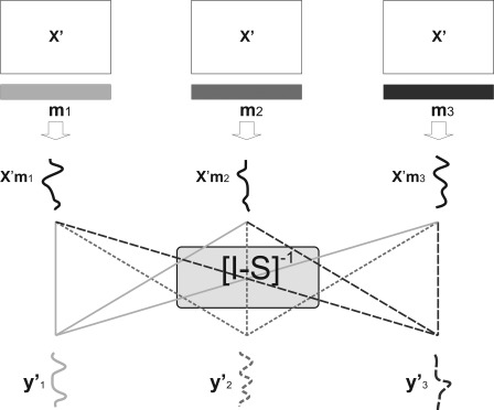
Graphical illustration of the generalization phase of the proposed model.

Formally:

$$\{\begin{array}{ccc}y{\prime }_1& =& \mathbf{X}\prime {\mathbf{m}}_1+\sum _{j\in {\mathrm{O}}_1}{m}_{1j}y{\prime }_j\\ y{\prime }_2& =& \mathbf{X}\prime {\mathbf{m}}_2+\sum _{j\in {\mathrm{O}}_2}{m}_{2j}y{\prime }_j\\ & \dots & \\ y{\prime }_n& =& \mathbf{X}\prime {\mathbf{m}}_n+\sum _{j\in {\mathrm{O}}_n}{m}_{nj}y{\prime }_j\end{array}$$ (10)

which in matrix notation, can be expressed as:

$$\mathbf{Y}\prime =\mathbf{X}\prime \mathbf{M}+\mathbf{Y}\prime \mathbf{S}$$ (11)

where the interaction matrix S is defined as:

$$S_{ij}=\{\begin{array}{ccc}0& if& i=j\\ m_{ij}& if& i\ne j\end{array}$$ (12)

Given the model used on the training data, the prediction $\mathbf{Y}\prime$ must satisfy Eq. (11), which means that the prediction on a new dataset can be expressed as a linear combination of the predictions $\stackrel{\sim }{\mathbf{Y}}\prime$ obtained with maps $\mathbf{M}$

$$\stackrel{\sim }{\mathbf{Y}}\prime =\mathbf{X}\prime \mathbf{M}$$ (13)

by means of the mixing matrix ${(\mathbf{I}-\mathbf{S})}^{-1}$:

$$\mathbf{Y}\prime =\mathbf{X}\prime \mathbf{M}{(\mathbf{I}-\mathbf{S})}^{-1}=\stackrel{\sim }{\mathbf{Y}}\prime {(\mathbf{I}-\mathbf{S})}^{-1}$$ (14)

A pseudo‐code implementation of the generalization phase is:

• Create the interaction matrix $\mathbf{S}$ containing $m_{ij}$ coefficients

• For each predictor i

  •     ○  Generate a prediction with data $\mathbf{X}\prime$ and ${\mathbf{m}}_i$: $\stackrel{\sim }{\mathbf{y}}{\prime }_i=\mathbf{X}\prime {\mathbf{m}}_i$

• Combine the predictions $\stackrel{\sim }{\mathbf{y}}{\prime }_i$ using mixing matrix ${\left[\mathbf{I}-\mathbf{S}\right]}^{-1}$

A MATLAB (http://www.mathworks.com) implementation of the proposed approach is available upon request to the corresponding author.

Datasets

Simulated fMRI dataset

We considered a set of simulations to examine and compare the performances of the proposed approach with those of standard MLKR and univariate multiple regression. We simulated a single fMRI slice consisting of 60 × 60 voxels, and considered a block design, with blocks and rest durations of 8 volumes, with 3 different experimental conditions. We modeled the BOLD response to the different experimental conditions by convolving a box‐car model of neural activity with a standard HRF function. These modeled responses were normalized between 0 and 1, and were used to simulate fMRI activity in several distinct areas with different weights. Gaussian i.i.d. noise with standard deviation ranging from 0.1 to 5 (on a non‐linear scale) was superimposed to the data. A variable amount of available volumes, ranging from 200 to 1000, was considered. The spatial and temporal profiles of a simulated dataset are illustrated in Figure 4. For each simulated dataset, we considered a threefold cross‐validation procedure, splitting the dataset in three parts, training on two of them and testing on the remaining part, considering the three possible combinations. For each cross‐validation procedure, we trained (1) our model, using Bayesian Linear Regression (BLR), (2) a standard MLKR, considering each target separately, again with BLR (3) univariate multiple regression (with Least‐Square estimation of the weights). We then compared the three approaches in terms of spatial detection power using the Area Under the Curve (AUC) of Receiver Operator Characteristic (ROC) curves, [Skudlarski et al., 1999]. ROC curves plot True Positive Rate versus False Positive rate values and their area (AUC) summarizes the curve by measuring its integral (with respect to False Positive Rate). The AUC can range between 0 and 1, and a large value denotes a good detection, with 1 being perfect detection, while smaller values denote poor accuracy, with 0.5 being the theoretical chance level. We also compared the three approaches in terms of generalization ability, by means of correlation between the predicted time course and the real one on the unseen test dataset. In the case of univariate regression, we predicted the time course in a new dataset by considering a weighted average of its voxels, with the weights being the univariate regression coefficients. Each dataset was generated 20 times, and the results were averaged across these iterations.

Figure 4.

Simulated fMRI datasets with three targets (a) Spatial layout of the maps associated with each target (b), targets time courses.

We furthermore compared the proposed approach with a simpler one, consisting of regressing out the remaining targets as confounds from the training data. The test data are not modified, since we assume no knowledge of the test targets.

PBAIC 2007 brain reading competition dataset

We considered the publicly available PBAIC 2007 (Pittsburgh Brain Activity Interpretation Competition) dataset (http://www.lrdc.pitt.edu/ebc/2007/competition.html). This dataset was used as a benchmark for several multivariate regression algorithms [Carroll et al., 2009; Chu et al., 2011b; Valente et al., 2011] to analyze and predict subject‐driven behavior in a virtual world. During the experiment, subjects had to navigate, collect objects, answer to cell phones giving them instructions, take pictures and avoid a threatening dog. Measurements of three subjects were collected on a Siemens Allegra 3T scanner in Pittsburgh University. Thirty‐four axial 3.5 mm thick slices were acquired parallel to the AC‐PC line using a reverse EPI sequence (TR = 1.75 s, TE = 25 ms, FOV = 210 mm, FA = 76^°). Structural data were acquired with 1 mm spatial resolution. Three functional runs, each lasting approximately 20 min, were collected per each subject, and were made available to the competition participants.

A set of ratings of subjects′ activity was associated with each functional run, based on eye movement as recorded by an eye‐tracking system, by virtual Reality logfiles and by subsequent subjective evaluation from the subjects. The ratings associated to the first two runs were made accessible to the participants, while the rating of the third run was used by the organizers to evaluate and rank the participants′ submissions. These ratings were related to different components of the subjects′ task such as audition (Instructions, Dog), vision (Body, Faces, Gender, and others), actions (Velocity, Hits, and others) and emotional valence (Arousal and Valence). Each rating was convolved with the standard double gamma model for hemodynamic response function and downsampled to match the functional scans temporal resolution. For more details on the competition, please refer to http://www.lrdc.pitt.edu/ebc/2007/competition.html and [Carroll et al., 2009; Chu et al., 2011b; Valente, et al. 2011].

In our approach to the PBAIC competition [Valente et al., 2011] we employed MLKR with Relevance Vector Machine (RVM) [Tipping, 2001] to predict unseen ratings based on fMRI data and we mapped the voxel′s relevance for each rating and examined the predictive maps of the different ratings. We analyzed the same dataset with our proposed algorithm focusing on audition and vision tasks (Instructions, Dog, Faces, Body, and Gender) and examined the difference between the predictive maps associated with a standard model with independent targets and the ones associated with the proposed method. We employed different kernel regression algorithms, including Relevance Vector Machine, Bayesian Linear Regression and Gaussian Processes. As the ratings of the third run are still unknown, we decided not to train a model on the two training runs together, as we could not compare the predictions obtained using the third functional run with the actual ratings; we instead used a cross‐validation approach, training on the first run and testing on the second (and vice versa), reporting the generalization in terms of correlation with the ratings of the (cross‐validation) test dataset. Furthermore, unlike in Valente et al. [2011], we did not consider any additional spatio‐temporal pre‐processing of the fMRI data, but considered only time‐series with high‐pass filtering of 3 cycles per time‐series.

To test for the significance of the accuracies, we conducted a non‐parametric permutation test, resampling the ratings and learning a model based on these new targets a thousand times. The ratings, which are based on eye‐tracking recordings convolved with an estimated of the HRF, exhibit, as well as BOLD time series, autocorrelations which would be neglected if the ratings were simply scrambled, leading to a wrong estimation of the empirical null distribution. We therefore implemented a wavelet resampling procedure based on Bullmore et al. [2001], decomposing each rating using a Daubechies mother wavelet with four vanishing moments into 7 levels, then resampling without replacement all the detail coefficients for each level and reconstructing the resampled time series in the time domain with the inverse wavelet transform. For each iteration, we scrambled each column of $\mathbf{Y}$ independently from the others. For this test we employed Bayesian Linear Regression, as it was the fastest of the used approaches. The scaling of the estimated maps changes at each permutation, and we corrected this by re‐scaling the estimated maps based on the variance of the times series and of the targets used at each iteration [see Supporting Information Appendix A, Eq. (11)] before estimating the empirical null distribution for each voxel.

RESULTS

Simulated fMRI Dataset

The results for the simulations are presented in Figure 5a. These simulations suggest that the proposed approach correctly recovers the spatial layout associated with the different targets, while maintaining the good generalization capabilities shown by traditional MLKR approaches.

Figure 5.

Results for the simulated dataset. (a) the first row depicts the ROC Area Under the Curve (AUC) as function of noise standard deviation (in logarithmic scale) for the proposed method, standard MLKR and univariate multiple regression. The second row shows the generalization on a new dataset, measured by correlation. (b) Comparison between the proposed approach and decorrelating the remaining targets from the training data. The first row depicts the ROC Area Under the Curve (AUC) as function of noise standard deviation (in logarithmic scale), the second row shows the generalization on a new dataset, measured by correlation.

AUC graphs indicate that, when the Signal to Noise (SNR) is low, i.e., when the noise standard deviation is large, multivariate regression algorithms tend to perform better than univariate multiple regression, due to their increased sensitivity to small effects. However, in the case of standard MLKR, negative activations, which result from the interaction with other maps as seen in Figure 1, affect the spatial sensitivity resulting in a loss of AUC. This effect is particularly relevant for the first target, where the negative activations are comparable in magnitude to the “true” ones.

Generalization (as assessed by correlation) graphs indicate that the generalization abilities of standard MLKR and of our approach are clearly similar, and they both outperform univariate multiple regression.

The comparison of the proposed approach and regressing out from the training data all the remaining targets is shown in Figure 5b. The results show that both methods achieve similar spatial accuracy (i.e., they are both effective in recovering the spatial layout of the sources), and that our approach outperforms the other in terms of generalization. This is due to the inclusion of the terms $m_{ij}$ in the model, which account for any shared variability between training data and remaining targets, which can then be exploited to achieve good generalization on new, unseen data.

PBAIC 2007 Dataset

We analyzed the PBAIC 2007 dataset with our approach and compared the results with the one obtained using multivariate regression considering one target at a time. The correlation coefficients between the predicted and the actual ratings considered are reported in Tables 1 and 2. The results of the model with separated targets are in Table 1, the ones obtained with the proposed approach are in Table 2. These values refer to Bayesian Linear Regression, while the correlation values obtained with Relevance Vector Machine and Gaussian Processes are reported in the Supporting Information. These correlation values were very similar to those obtained with BLR. Based on the permutation test, the accuracies obtained with Bayesian Linear Regression were all significant with P < 0.05: the correlations for all the targets, except Dog, were, for both methods and both runs, significant with p = 9·× 10⁻⁴; the correlation for the rating Dog was significant with p = 2 ×·10⁻³ for the prediction on run 2, and p = 0.023 for the prediction on run 1, for both methods.

Table 1.

Correlation between predictions and the actual ratings (in cross validation, from Run 1 to Run 2 and viceversa) for the model with separated (independent) targets

	Subject 1		Subject 13		Subject 14
	1 →2	2 → 1	1 →2	2 → 1	1 →2	2 → 1
Instructions	0.801	0.812	0.765	0.703	0.711	0.702
Dog	0.182	0.234	0.208	0.259	0.538	0.386
Faces	0.374	0.324	0.542	0.409	0.714	0.593
Body	0.521	0.575	0.516	0.344	0.592	0.570
Gender	0.346	0.341	0.329	0.261	0.374	0.359

Table 2.

Correlation between predictions and the actual ratings (in cross validation, from Run 1 to Run 2 and viceversa) for the proposed model

	Subject 1		Subject 13		Subject 14
	1 →2	2 → 1	1 →2	2 → 1	1 →2	2 → 1
Instructions	0.802	0.811	0.765	0.702	0.708	0.703
Dog	0.181	0.225	0.218	0.263	0.534	0.383
Faces	0.376	0.387	0.564	0.413	0.698	0.588
Body	0.466	0.582	0.533	0.339	0.520	0.541
Gender	0.253	0.351	0.290	0.264	0.332	0.406

On average, the ratings which are best predicted are Instructions and Faces. Furthermore, correlations are generally higher for Subject 14. Both these aspects are in line to what obtained on the third (test) run in the competition [Valente et al., 2011]. Accuracies obtained with our method where slightly higher than when using one target at a time in subject 13, while they were, to some extent, lower in subject 14. We compared the accuracies obtained with the two approaches, using a nonparametric Friedman test, which did not indicate any significant difference (with a Type I error level α of 0.05). Similarly, no significant difference was observed when using RVM or GP as kernel regression algorithms.

Predictive maps obtained with both methods were thresholded based on the non‐parametric (permutation) test. We considered each target separately, comparing the estimated (normalized) weights with the (normalized) weights obtained with the permuted labels. For each method and target, we considered each voxel′s empirical null distribution, fitted it with a Gaussian and calculated the P‐value associated with the estimated weights. We employed this fitting step as computational shortcut based on the assumption of normally distributed weights. These sets of P‐values were then thresholded using a False Discovery Rate (FDR) procedure [Genovese et al., 2002], to correct for multiple comparisons. All the maps were thresholded with q = 0.05. Maps associated with the different ratings based on the first run are shown in Figure 6 (Auditory features, Instructions and Dog) and Figure 7a,b (Visual features, Faces, Body, and Gender). The maps associated with each rating were standardized with z‐score transformation, where only the voxels that survived FDR correction are displayed.

Figure 6.

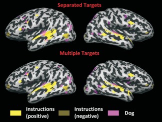
Predictive maps associated to the ratings Instructions and Dog, obtained on Subject 14, run 1, with Bayesian Linear Regression. The maps obtained with standard MLKR are shown in the top panel, while the ones obtained with the proposed method, learning all the five ratings together are shown in the bottom panel. The maps are corrected with FDR, q = 0.05. [Color figure can be viewed in the online issue, which is available at http://wileyonlinelibrary.com.]

Figure 7.

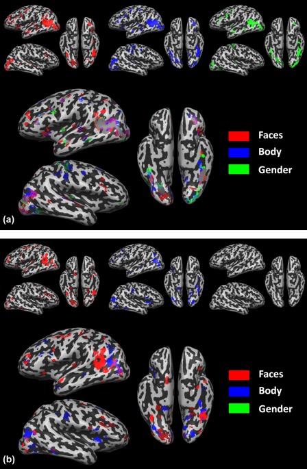
Predictive maps associated to the ratings Faces, Body and Gender obtained on Subject 14, run 1, with Bayesian Linear Regression using (a) standard MLKR (b) the proposed approach. All the maps are corrected with FDR, q = 0.05. [Color figure can be viewed in the online issue, which is available at http://wileyonlinelibrary.com.]

The patterns associated with auditory features are similar in both situations (separated targets and considering interactions between targets), indicating some degree of overlap between the maps associated with Instructions and the one associated with Dog in auditory areas. The distributed pattern associated with Instructions is spread through the temporal lobes in regions which are typically associated with processing of speech and language (seemingly with higher intensity in the left hemisphere), with a negative contribution from Middle Temporal Gyrus (MTG). Such contribution is not due to interactions between ratings. In fact, when including the visual ratings which have a large contribution from MTG, the spatial layout of the negative contributions to Instructions does not change.

The patterns associated to visual features, on the other hand, show some noteworthy differences when learning a target independently of the others (Fig. 7a) or when learning all of them together (Fig. 7b). When considering targets separately, the maps associated to the visual ratings are indeed considerably similar to each other, exhibiting a large overlap mainly in the left hemisphere, in the MTG in the Middle Occipital Gyrus (MoG) and in the occipital cortex. However, when considering all the targets together, with the model proposed in this work, the predictive maps associated with the visual features do not show such close resemblance, but they show distributed, and yet overlapping, patterns in similar regions. Whereas the predictive map associated to Faces does not seem particularly affected by the inclusion of the other ratings, both the maps associated with Body and Gender show large differences when compared with their counterpart in Figure 7a. The predictive map associated with Body preserves its localization in both MTG/MoG and the occipital cortex, but it does not closely follow the one associated to Faces. The map associated with Gender, on the other hand, does not survive the multiple comparison correction, indicating that no reliable pattern can be associated with such rating.

The correlations between the actual ratings and the ones obtained with the maps estimated with separated targets (Fig. 7a), with the maps estimated using Eq. (7) (Fig. 7b) $\stackrel{\sim }{\mathbf{Y}}=\mathbf{X}M$, and with the prediction based on Eq. (14) $\mathbf{Y}=\mathbf{X}M{(\mathbf{I}-\mathbf{S})}^{-1}$, are show in Table 3. Furthermore, for each prediction we considered the actual rating and projected it on the orthogonal subspace of the other (actual) ratings, evaluated the correlation with the predictions $\stackrel{\sim }{Y}=\mathbf{X}M$ based on the estimated maps. As expected, the predictions of Instructions and Dog is similar for all cases. Faces shows a small improvement when including the information contained in $\mathbf{S}$, while Body and Gender show the largest increment in generalization, with Gender changing from a negative correlation (−0.19) to a positive one (0.33).

Table 3.

Correlation between prediction and actual ratings for Subject 14, from run 1 to 2, considering (1) the standard MLKR with separated targets (Fig. 7a), (2) the maps estimated with the proposed model [Fig. 7b and Eq. (13)], (3) the same prediction as in (2), after the actual rating has been decorrelated from the others, (4) the predictions using the information in matrix S [Eq. (14)] and the original ratings

	Separated predictors	$\stackrel{\sim }{\mathbf{Y}}=\mathbf{X}M$	$\stackrel{\sim }{\mathbf{Y}}=\mathbf{X}M$ on residual targets	$\mathbf{Y}=\mathbf{X}M{(\mathbf{I}-\mathbf{S})}^{-1}$
Instructions	0.711	0.709	0.686	0.708
Dog	0.538	0.531	0.522	0.534
Faces	0.714	0.641	0.513	0.698
Body	0.592	0.319	0.302	0.520
Gender	0.374	−0.187	0.038	0.332

For each rating, we furthermore evaluated the relative contribution to the predicted rating $\mathbf{Y}$ of the a) prediction based on the map associated with the rating ${\stackrel{\sim }{\mathbf{y}}}_i=\mathbf{X}{\mathbf{m}}_i$ and of b) the predictions based on the remaining maps ${\stackrel{\sim }{\mathbf{Y}}}_{O_i}=\mathbf{X}{\mathbf{M}}_{O_i}$. Both the predictions $\mathbf{Y}$ and $\stackrel{\sim }{\mathbf{Y}}$ were first standardized with a z‐score transformation and then each column of $\mathbf{Y}$ was fit using $\stackrel{\sim }{\mathbf{Y}}$. For each prediction, we considered the square of the regression coefficients associated with ${\stackrel{\sim }{\mathbf{y}}}_i$ and the sum of squares of the coefficients associated with ${\stackrel{\sim }{\mathbf{Y}}}_{O_i}$ and normalized them such that their sum is one. The values are reported in Table 4, which indicates, once again, that the prediction of Gender is largely dependent on the other ratings, rather than on the associated predictive map

Table 4.

Relative contribution of the map associated to the target and of the other maps in the prediction of the ratings

Prediction	Contribution from ${\stackrel{\sim }{\mathbf{y}}}_i=\mathbf{X}{\mathbf{m}}_i$	Contribution from ${\stackrel{\sim }{\mathbf{Y}}}_{O_i}=\mathbf{X}{\mathbf{M}}_{O_i}$
Instructions	0.998	0.002
Dog	0.979	0.021
Faces	0.713	0.287
Body	0.776	0.224
Gender	0.118	0.882

DISCUSSION

In this work we have shown how to map brain activity with predictive models, such as those provided by Multivariate Linear Regression, whose maps may be of difficult interpretation in the presence of multiple targets. This is a relevant issue in fMRI, as ignoring this aspect of the problem does not harm the generalization on unseen datasets, but it confounds the predictive maps associated with the learnt model, making it troublesome to interpret the findings or to draw conclusions based on the relevance that difference areas have in the overall prediction.

With our method a model is still learnt for each target (or label), but differently from the standard formulation, additional features accounting for the presence of the other targets are included in the training. The predictive maps associated with this formulation do not suffer from the same drawbacks as when considering the targets independently, and the weights of the additional features included in the model are then used to generate a prediction on an unseen dataset.

The estimation of the maps is similar to what proposed in Friston et al. [2008], where the effect of neural activity associated to the other targets is regressed out as confound. However, unlike Friston et al. [2008], we do not assume knowledge of any of the test targets. Thus, it is not possible to remove the effects of confound targets from the whole dataset (or from training and testing data separately) and then perform inference on the residual. Instead we estimate both maps and interaction coefficients solely on the training dataset and perform prediction (and thus inference) on the original targets, rather than on the residuals.

The prediction of a target consists of two parts [see Eq. (14) and Fig. 3]: what is predicted by the map associated with the studied target, and what is predicted by the other maps, with the weighting provided in ${\left(\mathbf{I}-\mathbf{S}\right)}^{-1}$. Whereas the validation of the model is performed examining generalization on the test targets, it is useful to characterize the contribution of both terms to the prediction by means of relative contribution, as illustrated in Table 4.

We have validated the model on simulations and on the publicly available PBAIC 2007 fMRI dataset. In Valente et al. [2011] we focused on the contribution of different networks of areas in predicting ratings using the standard regression model [Eq. (3)]. The results highlighted a large similarity between the predictive maps of the ratings Faces, Body, and Gender, (Fig. 7a) and an overlap between negative activations predictive of rating Instruction and the mentioned visual features (Fig. 6, top panel). With the proposed approach we could determine whether such overlap was due to similar neural processing or to the interaction between ratings, which is not possible with the standard framework of multivariate regression.

The formulation of this work is based on the assumption that the variability of the targets can be captured adequately by linear models. The kernels employed in this work [see Eq.(5)] allow a linear formulation of the problem, making it possible to remove the effect of the others targets by means of subspace projection. With non‐linear models, the formulation proposed in this work would not hold anymore. However, mapping of brain activity with non‐linear models is not straightforward, and non‐linear models are seldom employed in MVPA for fMRI, where the amount of features is considerably larger than the amount of samples [Cox and Savoy, 2003]. Investigating whether the proposed framework could be generalized to regression with non‐linear kernel making use of the approaches proposed in [Golland et al., 2005; Rasmussen et al., 2011], is an interesting research direction.

The current formulation is based on kernel methods such as Kernel Ridge Regression, Bayesian Linear Regression, Relevance Vector Machine and Gaussian Processes. These approaches are attractive from a computational perspective, as they project the data onto a lower dimensional space, before estimating a regularized model. Several approaches, however, that do not require the use of kernels, have been proposed in literature to deal with the large dimensions of fMRI data, including SVD‐based dimension reduction [Hastie et al., 2004], L1‐norm regularization (LASSO) and combined L1 and L2‐norm regularization (Elastic Net) [Carroll et al., 2009; Hastie et al., 2009; Tibshirani, 1996; Zou and Hastie 2005]. L1‐norm regularization enforces sparsity in the feature space, performing joint model estimation and feature selection (similarly to Sparse Bayesian Learning [Li et al., 2002; Tipping, 2001], which is based on an identity kernel $\mathbf{K}=\mathbf{X}$). The use of such models would not solve the problem of mapping voxel relevance, as seen in the example, since the confounding of maps does not come from the inclusion of unnecessary voxels, but arises from the presence of areas which are linked to more than one target, and would survive the pruning process. Given the fact that also L1‐norm based approaches usually employed in fMRI data analysis are linear (in the voxel space), it is reasonable to assume that the formulation presented in Eq. (7) would also help recover correct spatial patterns of activity and good generalization when the maps are estimated with such algorithms rather than with MLKR. However, the formulation we have proposed here is not specifically designed for such approaches and it has not been tested in this work. It would be interesting to determine for which multivariate regression approaches the proposed method works satisfactorily.

Predictive models make few assumptions, giving more emphasis on the ability to generalize on unseen dataset than on making explicit parametric inference on the weights of the model. By using regularization, which “simplifies” the learning models according to the available examples, such algorithms can achieve good generalization performances on unseen data, which is a crucial aspect and serves as an “empirical” validation of the model. This step provides an important safety check on the model employed, protecting against overfitting [Bishop, 2006]. However, since most of these algorithms have been designed for prediction, rather than for inference, it is more troublesome to assess the confidence on each parameter estimate. Consider the example of Ridge Regression (and similarly of Bayesian Linear Regression or Gaussian Processes using a covariance matrix with one hyperparameter). In this model, the variance of the parameter estimates is reduced by the penalization factor, at the expenses of an increased bias [Hoerl and Kennard, 1970a,1970b], determining the amount of regularization based on the training data. For such a model, the parameter distribution is unknown; therefore, no parametric statistic can be employed. Permutation tests remain a more viable option, and the current increases in computational power make them an increasingly accessible statistical assessment tool. In the current study we have employed False Discovery Rate (FDR) correction for the multivariate maps estimated with MLKR on the PBAIC dataset. An interesting research direction is the comparative study of different statistical correction procedures that include topological information of the multivariate maps, such as cluster‐size threshold estimation [Forman et al., 1995] and topological FDR [Chumbley et al., 2010].

It is interesting to relate the proposed method, and in general multivariate regression, to MVPA classification approaches [Norman et al., 2006]. Despite the most obvious difference, which is that classification algorithms deal with discrete labels and regression algorithms with continuous ones—that in turn leads to different error measures and therefore algorithms [Bishop, 2006]—both these techniques investigate associations between brain states and cognitive processes. Consider a typical controlled fMRI experiment, where different sensory or cognitive tasks are performed in a randomized sequence of blocks or events. A typical classification approach summarizes the information associated with each event (or block) in a multidimensional feature vector, and then find suitable weights in this multidimensional space that reliably discriminate between the two (or more) experimental conditions [Norman et al., 2006]. This decoding framework serves the purpose of detecting small, and yet consistent, effects which may be overlooked with a univariate approach. Most of the algorithms successfully employed to decode brain states are based on discriminative models, which efficiently solve the problem of providing a rule to distinguish between two classes, without trying to characterize the classes in themselves. This also implies that the predictive maps estimated with MVPA do not suffer from the drawbacks we have discussed in this work, if only two conditions are considered. An MVPA analysis to discriminate between the two conditions coded with the two targets in Figure 1 would result in a discriminative map containing areas S1, S2, and S4, with areas S1 and S4 having opposite sign to area S2. However, when three or more conditions are considered, a one‐vs‐all classification approach could potentially result in interpretative problems, if the discriminative map of a condition versus all the others is used to infer condition specific brain behavior.

The nature of multivariate regression, on the other hand, allows researchers to benefit from the increased sensitivity of multivariate methods while dealing with experiments with less strict settings (and thus more realistic), such as those employed in the PBAIC competition, or while combining single trial EEG peaks and power modulations and fMRI. In such cases MVPA approaches are not suitable and multivariate regression should be used. The question remains, however, whether multivariate regression can be employed in a similar way as MVPA to discriminate between different conditions, drawing a parallel to the contrast used in standard univariate analyses. Chu et al. [2011a] moved along this direction showing how to use MLKR to perform multi‐class classification, comparing on several experiments the performances of an SVM‐based classifier with a MLKR‐based classifier. This approach, however, did not explicitly model the difference between brain states in two or more conditions, but rather estimated a multivariate map for each class assigning a new trial to a class based on template matching procedures. An interesting research direction is to investigate the possibility to directly learn contrasts with multivariate regression, accounting for confounds such as motion by including correction parameters.

Supporting information

Supporting Information Appendix.

REFERENCES

- Bishop C (2006): Pattern Recognition and Machine Learning. Springer, New York. [Google Scholar]
- Bullmore E, Long C, Suckling J, Fadili J, Calvert G, Zelaya F, Carpenter TA, Brammer M (2001): Colored noise and computational inference in neurophysiological (fMRI) time series analysis: resampling methods in time and wavelet domains. Hum Brain Mapp 12:61–78. [DOI] [PMC free article] [PubMed] [Google Scholar]
- Carroll MK, Cecchi GA, Rish I, Garg R, Rao AR (2009): Prediction and interpretation of distributed neural activity with sparse models. Neuroimage 44:112–122. [DOI] [PubMed] [Google Scholar]
- Chu C, Mourao‐Miranda J, Chiu YC, Kriegeskorte N, Tan G, Ashburner J (2011a): Utilizing temporal information in fMRI decoding: classifier using kernel regression methods. Neuroimage 58:560–571. [DOI] [PMC free article] [PubMed] [Google Scholar]
- Chu C, Ni Y, Tan G, Saunders CJ, Ashburner J (2011b): Kernel regression for fMRI pattern prediction. Neuroimage 56:662–673. [DOI] [PMC free article] [PubMed] [Google Scholar]
- Chumbley J, Worsley K, Flandin G, Friston KJ (2010): Topological FDR for neuroimaging. NeuroImage 49:3057–3064. [DOI] [PMC free article] [PubMed] [Google Scholar]
- Cohen JR, Asarnow RF, Sabb FW, Bilder RM, Bookheimer SY, Knowlton BJ, Poldrack RA (2011): Decoding continuous variables from neuroimaging data: Basic and clinical applications. Front Neurosci 5:75. [DOI] [PMC free article] [PubMed] [Google Scholar]
- Cox DD, Savoy RL (2003): Functional magnetic resonance imaging (fMRI) “brain reading”: Detecting and classifying distributed patterns of fMRI activity in human visual cortex. Neuroimage 19(2 Part 1):261–270. [DOI] [PubMed] [Google Scholar]
- De Martino F, Valente G, de Borst AW, Esposito F, Roebroeck A, Goebel R, Formisano E (2010): Multimodal imaging: An evaluation of univariate and multivariate methods for simultaneous EEG/fMRI. Magn Reson Imaging 28:1104–1112. [DOI] [PubMed] [Google Scholar]
- De Martino F, de Borst AW, Valente G, Goebel R, Formisano E (2011): Predicting EEG single trial responses with simultaneous fMRI and relevance vector machine regression. Neuroimage 56:826–836. [DOI] [PubMed] [Google Scholar]
- Duchesne S, Caroli A, Geroldi C, Collins DL, Frisoni GB (2009): Relating one‐year cognitive change in mild cognitive impairment to baseline MRI features. Neuroimage 47:1363–1370. [DOI] [PubMed] [Google Scholar]
- Forman SD, Cohen JD, Fitzgerald M, Eddy WF, Mintun MA, Noll DC (1995): Improved assessment of significant activation in functional magnetic resonance imaging (fMRI): Use of a cluster‐size threshold. Magn Reson Med 33:636–647. [DOI] [PubMed] [Google Scholar]
- Formisano E, De Martino F, Valente G (2008): Multivariate analysis of fMRI time series: Classification and regression of brain responses using machine learning. Magn Reson Imaging 26:921–934. [DOI] [PubMed] [Google Scholar]
- Franke K, Ziegler G, Kloppel S, Gaser C (2010): Estimating the age of healthy subjects from T1‐weighted MRI scans using kernel methods: Exploring the influence of various parameters. Neuroimage 50:883–892. [DOI] [PubMed] [Google Scholar]
- Friston KJ, Frith CD, Frackowiak RS, Turner R (1995a): Characterizing dynamic brain responses with fMRI: a multivariate approach. Neuroimage 2(2):166–72. [DOI] [PubMed] [Google Scholar]
- Friston KJ, Holmes A, Worsley KJ, Poline JB, Frith CD, Frackowiak RS (1995b): Statistical Parametric Maps in functional imaging: a general linear approach. Hum Brain Mapp 2:189–210. [Google Scholar]
- Friston KJ, Fletcher P, Josephs O, Holmes A, Rugg MD, Turner R (1998): Event‐related fMRI: Characterizing differential responses. Neuroimage 7:30–40. [DOI] [PubMed] [Google Scholar]
- Friston KJ, Chu C, Mourão‐Miranda J, Hulme O, Rees G, Penny W, Ashburner J (2008): Bayesian decoding of brain images. NeuroImage 39:181–205. [DOI] [PubMed] [Google Scholar]
- Genovese CR, Lazar NA, Nichols T (2002): Thresholding of statistical maps in functional neuroimaging using the false discovery rate. Neuroimage 15:870–878. [DOI] [PubMed] [Google Scholar]
- Golland P, Grimson WEL, Shenton ME, Kikinis R (2005): Detection and analysis of statistical differences in anatomical shape. Med Image Anal 9:69–86. [DOI] [PMC free article] [PubMed] [Google Scholar]
- Hastie T, Tibshirani R (2004): Efficient quadratic regularization for expression arrays. Biostatistics 5:329–340. [DOI] [PubMed] [Google Scholar]
- Hastie T, Tibshirani R, Friedman JH (2009): The elements of statistical learning: Data mining, inference and prediction. New York: Springer‐Verlag. [Google Scholar]
- Haxby JV, Gobbini MI, Furey ML, Ishai A, Schouten JL, Pietrini P (2001): Distributed and overlapping representations of faces and objects in ventral temporal cortex. Science 293:2425–2430. [DOI] [PubMed] [Google Scholar]
- Hoerl A, Kennard R (1970a): Ridge regression: Applications to nonorthogonal problems. Technometrics 12:69–82. [Google Scholar]
- Hoerl A, Kennard R (1970b): Ridge regression: Biased estimation for nonorthogonal problems. Technometrics 12:55–67. [Google Scholar]
- Kherif F, Poline JB, Flandin G, Benali H, Simon O, Dehaene S, Worsley KJ (2002): Multivariate model specification for fMRI data. Neuroimage 16:1068–1083. [DOI] [PubMed] [Google Scholar]
- Kiebel SJ, Goebel R, Friston KJ (2000): Anatomically informed basis functions. NeuroImage 11:656–667. [DOI] [PubMed] [Google Scholar]
- Kjems U, Hansen LK, Anderson J, Frutiger S, Muley S, Sidtis J, Rottenberg D, Strother SC (2002): The quantitative evaluation of functional neuroimaging experiments: Mutual information learning curves. Neuroimage 15:772–786. [DOI] [PubMed] [Google Scholar]
- Kriegeskorte N, Goebel R, Bandettini P (2006): Information‐based functional brain mapping. Proc Natl Acad Sci USA 103:3863–3868. [DOI] [PMC free article] [PubMed] [Google Scholar]
- Lautrup B, Hansen L, Law I, Mørch N, Svarer C, Strother S (1994): Massive weight sharing: A cure for extremely ill‐posed problems. In: Proceedings of the Workshop on Supercomputing in Brain Research: From Tomography to Neural Networks. Ulich, Germany: World Scientific. pp 137–148.
- Li Y, Campbell C, Tipping M (2002): Bayesian automatic relevance determination algorithms for classifying gene expression data. Bioinformatics 18:1332–1339. [DOI] [PubMed] [Google Scholar]
- Marquand A, Howard M, Brammer M, Chu C, Coen S, Mourao‐Miranda J (2010): Quantitative prediction of subjective pain intensity from whole‐brain fMRI data using Gaussian processes. Neuroimage 49:2178–2189. [DOI] [PubMed] [Google Scholar]
- McIntosh AR, Bookstein FL, Haxby JV, Grady CL (1996): Spatial pattern analysis of functional brain images using partial least squares. Neuroimage 3(3 Part 1):143–157. [DOI] [PubMed] [Google Scholar]
- Norman KA, Polyn SM, Detre GJ, Haxby JV (2006): Beyond mind‐reading: multi‐voxel pattern analysis of fMRI data. Trends Cogn Sci 10:424–430. [DOI] [PubMed] [Google Scholar]
- Penny WD, Trujillo‐Bareto N, Friston KJ (2005): Bayesian fMRI time series analysis with spatial priors. NeuroImage 24:350–362. [DOI] [PubMed] [Google Scholar]
- Pereira F, Mitchell T, Botvinick M (2009): Machine learning classifiers and fMRI: A tutorial overview. NeuroImage 45:S199–S209. [DOI] [PMC free article] [PubMed] [Google Scholar]
- Rasmussen CE, Williams C (2006): Gaussian processes for machine learning. The MIT Press, Cambridge (MA). [Google Scholar]
- Rasmussen PM, Madsen KH, Lund TE, Hansen LK (2011): Visualization of nonlinear kernel models in neuroimaging by sensitivity maps. Neuroimage 55:1120–1131. [DOI] [PubMed] [Google Scholar]
- Skudlarski P, Constable RT, Gore JC (1999): ROC analysis of statistical methods used in functional MRI: Individual subjects. Neuroimage 9:311–329. [DOI] [PubMed] [Google Scholar]
- Smith M, Pütz B, Auer D, Fahrmeir L (2003): Assessing brain activity through spatial bayesian variable selection. NeuroImage 20:802–815. [DOI] [PubMed] [Google Scholar]
- Stonnington CM, Chu C, Kloppel S, Jack CR Jr, Ashburner J, Frackowiak RS (2010): Predicting clinical scores from magnetic resonance scans in Alzheimer′s disease. Neuroimage 51:1405–1413. [DOI] [PMC free article] [PubMed] [Google Scholar]
- Tibshirani R (1996): Regression shrinkage and selection via the lasso. J R Stat Soc Ser B 58:267–288. [Google Scholar]
- Tipping M (2001): Sparse bayesian learning and the relevance vector machine. J Mach Learn Res 1:211–244. [Google Scholar]
- Valente G, De Martino F, Esposito F, Goebel R, Formisano E (2011): Predicting subject‐driven actions and sensory experience in a virtual world with relevance vector machine regression of fMRI data. Neuroimage 56:651–661. [DOI] [PubMed] [Google Scholar]
- Wang Y, Fan Y, Bhatt P, Davatzikos C (2010): High‐dimensional pattern regression using machine learning: From medical images to continuous clinical variables. Neuroimage 50:1519–1535. [DOI] [PMC free article] [PubMed] [Google Scholar]
- Woolrich MW, Behrens TE, Beckmann CF, Smith SM (2005): Mixture models with adaptive spatial regularization for segmentation with an application to FMRI data. IEEE Trans Med Imaging 24:1–11. [DOI] [PubMed] [Google Scholar]
- Worsley KJ, Poline JB, Friston KJ, Evans AC (1997): Characterizing the response of PET and fMRI data using multivariate linear models. Neuroimage 6:305–319. [DOI] [PubMed] [Google Scholar]
- Zou H, Hastie T (2005): Regularization and variable selection via the elastic net. J R Stat Soc Ser B 67:301–320. [Google Scholar]
Associated Data
This section collects any data citations, data availability statements, or supplementary materials included in this article.
Supplementary Materials