Regional variations in vascular density correlate with resting‐state and task‐evoked blood oxygen level‐dependent signal amplitude

Abstract

Functional magnetic resonance imaging (fMRI) has become one of the primary tools used for noninvasively measuring brain activity in humans. For the most part, the blood oxygen level‐dependent (BOLD) contrast is used, which reflects the changes in hemodynamics associated with active brain tissue. The main advantage of the BOLD signal is that it is relatively easy to measure and thus is often used as a proxy for comparing brain function across population groups (i.e., control vs. patient). However, it is particularly weighted toward veins whose structural architecture is known to vary considerably across the brain. This makes it difficult to interpret whether differences in BOLD between cortical areas reflect true differences in neural activity or vascular structure. We therefore investigated how regional variations of vascular density (VAD) relate to the amplitude of resting‐state and task‐evoked BOLD signals. To address this issue, we first developed an automated method for segmenting veins in images acquired with susceptibility‐weighted imaging, allowing us to visualize the venous vascular tree across the brain. In 19 healthy subjects, we then applied voxel‐based morphometry (VBM) to T1‐weighted images and computed regional measures of gray matter density (GMD). We found that, independent of spatial scale, regional variations in resting‐state and task‐evoked fMRI amplitudes were better correlated to VAD compared to GMD. Using a general linear model (GLM), it was observed that the bulk of regional variance in resting‐state activity could be modeled by VAD. Cortical areas whose resting‐state activity was most suppressed by VAD correction included Cuneus, Precuneus, Culmen, and BA 9, 10, and 47. Taken together, our results suggest that resting‐state BOLD signals are significantly related to the underlying structure of the brain vascular system. Calibrating resting BOLD activity by venous structure may result in a more accurate interpretation of differences observed between cortical areas and/or individuals. Hum Brain Mapp 35:1906–1920, 2014. © 2013 Wiley Periodicals, Inc.

INTRODUCTION

During the last two decades, several functional magnetic resonance imaging (fMRI) studies have been carried out using the blood oxygenation level‐dependent (BOLD) contrast to map brain function in humans performing a task (T‐fMRI) and/or during rest (RS‐fMRI). Using the variation of the oxy/deoxygenated blood ratio and blood volume in the brain following neural activation, the BOLD signal is a surrogate measure of neural activity, reflecting hemodynamic changes caused by a complex interaction of cerebral blood flow (CBF), cerebral blood volume (CBV), and cerebral metabolic rate of oxygen (CMRO₂) [Attwell and Iadecola, 2002; Attwell et al., 2010; Bandettini et al., 1993; Biswal et al., 1995; Fox and Raichle, 2007, 1986; Nair, 2005; Ogawa et al., 1993; Uludağ et al., 2009]. BOLD contrast at fields below 4T mainly arises from changes in oxygenation in venules and veins lying relatively close to the site of increased neuronal activity [Song et al., 1996; Turner, 2002] and studies in animals have demonstrated that both stimulus‐induced and spontaneous changes in BOLD contrast are tightly linked to corresponding changes in neural activity [Logothetis, 2002; Pan et al., 2011; Schölvinck et al., 2010]. However, inferring the magnitude (i.e., amplitude) of neural activity from BOLD fluctuations is not straight forward. This is because the magnitude of a BOLD fMRI response is weighted by baseline CBV_venous and stimulus‐induced venous oxygenation level changes [Kim and Ogawa, 2012]. Cortical areas with higher baseline CBV_venous values will therefore show a higher BOLD response [Moon et al., 2013; Yu et al., 2012; Zhao et al., 2006] even if underlying oxygen level and neural changes are the same [Davis et al., 1998]. Interestingly, a recent study demonstrated that the amplitude of baseline (resting‐state [RS]) BOLD activity is also highly correlated to its task‐evoked modulation [Kannurpatti et al., 2012]. One possible explanation for this is that baseline BOLD activity is directly related to inherent vascular venous structure, which is known to vary considerably across human cortex [Duvernoy et al., 1981]. Thus, comparing task‐related BOLD responses between areas and/or individuals is difficult to interpret [Ances et al., 2008; Buxton et al., 2004], given that regional variations in the brain venous network may predetermine the ability to detect reliable BOLD signals [Ekstrom, 2010] and thus explain the reason why certain brain areas are routinely found to be “activated” across a wide range of cognitive tasks [Gusnard and Raichle, 2001], whereas areas with an insufficient vascular network, that is low vascular density (VAD), may not produce functional response at all [Harrison et al., 2002]. This could be owing to the fact that areas with higher VAD reflect an increased signal‐to‐noise ratio of the BOLD signal and as a result increase the chances of detecting a difference between experimental conditions [Weber et al., 2008]. It is therefore important to fully characterize whole‐brain venous vasculature prior to interpreting BOLD responses between brain areas and/or individuals.

The issue of venous vasculature and how it complicates the interpretation of BOLD amplitude is not new. Menon et al. [1993] were one of the first to show that vessels (and therefore voxels with a high fractional blood volume) show the largest BOLD signal changes. This was also observed in subsequent modeling studies of cortical hemodynamics [Bandettini and Wong, 1995; Ogawa et al., 1993]. As it is now well accepted that BOLD signals are most pronounced near large vessels [Bianciardi et al., 2011; Hoogenraad et al., 1999; Kim et al., 1994; Leontiev and Buxton, 2007], it is plausible that BOLD signals in heavily vascularized areas will appear artificially amplified compared to other areas with less dense vascularization [Bandettini, 2012]. Indeed, studies in animal and humans have shown that variations in VAD within a single cortical area (e.g., auditory cortex) are tightly linked to stimulus‐evoked response magnitude [Casciaro et al., 2008; Hall et al., 2002]. Although these studies have quantified the effects of vasculature on BOLD activity within a single area, it is unclear how whole‐brain vessel architecture affects widespread fMRI activity patterns encompassing multiple brain areas. Addressing this is particularly important, given the growing number of RS fMRI studies which use the amplitude of spontaneous BOLD signals to infer the magnitude of neural activity [Qi et al., 2012] and compare it across different cortical areas and populations [Jiao et al., 2011; Wang et al., 2011; Xi et al., 2012; Zang et al., 2007].

Early attempts aimed at suppressing the effects of venous structure on BOLD signals were made by using a hypercapnic challenge (breathing CO₂) to identify and correct the contribution from large veins [Bandettini and Wong, 1997; Davis et al., 1998]. Later studies used a similar methodology to correct for population differences in vasculature [Thomason et al., 2007], and more recent high‐field (7T) study used vessel‐size imaging to characterize its effect on BOLD signal amplitude [Jochimsen et al., 2010]. However, typical experiments involving hypercapnic challenges (breathing CO₂ or breath holding) can require relatively long scan times [Handwerker et al., 2012] and may be difficult or even dangerous to implement in certain patient groups [Brevard et al., 2003; Bright et al., 2009]. Thus, a more direct approach to imaging the venous vasculature and removing its contribution to the BOLD signal would be useful, particularly for clinical fMRI studies at 1.5T which are known to be very susceptible to tissue containing venules and large veins [Seiyama et al., 2004].

In this study, we use a novel method to reinvestigate the well‐known, yet often neglected impact of cerebral vascularization on the interpretation of RS and task‐evoked BOLD signals. We first developed an automated approach of segmenting vessels based on susceptibility‐weighted images (SWIs) from which we then compute regional measures of VAD at various spatial scales. We found that regional variations in VAD could explain a significant portion of amplitude variations in RS and task‐evoked BOLD fluctuations. These results therefore highlight the importance of incorporating vessel structure when comparing fMRI signals between different areas and subjects.

METHODS

Subjects

Nineteen (19) right‐handed subjects (four females, ages, 20–33 years) were recruited for the study. All subjects were native French speakers and had no psychiatric or neurologic symptoms at the time of scanning or in the past. This study was performed according to the guidelines of the Internal Review Board of the Centre Hospitalier Universitaire de Sherbrooke (CHUS).

Image Acquisition

Imaging data were acquired using a 1.5T Siemens Magnetom (Vision). Each session started with separate fMRI acquisitions during a task (T‐fMRI) and at rest (RS‐fMRI), followed by a SWI acquisition and finally an anatomical T1‐weighted 1 mm isotropic (TR/TE 6.57/2.52 ms) acquisition.

Task‐Induced fMRI

Continuous imaging of brain activity was done using a standard echo planar imaging (EPI) sequence. Thirty axial image slices of 3 mm thickness (no gap) were obtained with a 64 × 64 matrix, field of view 240 mm, TR/TE 3864/40 ms. Voxel size was 3.75 × 3.75 × 3 mm. Data were acquired in a box‐car format, with subjects alternating between baseline and task conditions via short auditory cues. Subjects performed 11 alternating epochs of 30 s each, resulting in a total scan time of 5 min and 30 s. For the task, subjects were asked to silently (eyes closed) perform Roland's Hometown Walking Task [Roland et al., 1987]. Prior to scanning, each subject chose five familiar walking routes. The majority of the subjects chose their home residence as starting point followed by commonly travelled points such as a grocery store, pharmacy, and pubs. They were not required to find the fastest, easiest, or most common route, only instructed to “follow the most familiar route.” Familiarity with each destination was assured before scanning, and all subjects were debriefed afterward to ensure compliance. As a baseline condition, subjects were asked to silently count backward by 3 from 271 at a rate of about one number per second. To prevent movement artifacts, subjects were instructed to refrain completely from talking throughout the scanning period.

Resting‐State Functional Magnetic Resonance Image

RS‐fMRI data were acquired using the same imaging parameters as the T‐fMRI. The subjects were instructed to remain still, close their eyes, and not fall asleep. The total scan time for RS‐fMRI was 3 min.

Susceptibility‐Weighted Imaging

Images of the brain vasculature were acquired using a SWI sequence [Haacke et al., 2006]. Slices of 1.6 mm thickness were obtained with a 320 × 260 acquisition matrix, TR/TE of 49/40 ms. Voxel size was 0.719 × 0.719 × 1.6 mm.

Image Processing

The main purpose of this study was to investigate the relationship between structural features of the brain (gray matter [GM], white matter [WM], and veins) and the amplitude of the BOLD signal obtained with fMRI. For this, we used AFNI [Cox, 1996] (http://afni.nimh.nih.gov/afni) for functional analysis, along with FSL [Smith et al., 2004; Woolrich et al., 2009] (http://www.fmrib.ox.ac.uk/fsl) and the SPM8‐VBM8 toolkit (http://dbm.neuro.uni-jena.de/vbm/) for structural analysis. Further analysis was performed using in‐house routines developed in MATLAB (Mathworks, Natick, USA).

Structural Analysis

Voxel‐based morphometry

The brain was first extracted from the skull using the AFNI command 3dSkullStrip and then subdivided into structural classes (GM, WM, and cerebrospinal fluid) using the VBM method implemented in SPM8‐VBM8 (http://dbm.neuro.uni-jena.de/vbm/). As a result, each voxel had a probability of belonging to each structural class, and those whose probability exceeded 50% (threshold based on the previous studies [Zuo et al., 2010]) were isolated and used to create binary masks of GM and WM.

Vasculature segmentation

Veins and sinuses were automatically segmented from the SWI volumes using the method developed by Descoteaux et al. [2004, 2008] for black blood contrast modalities based on the vesselness measure of Frangi et al. [1998]. Briefly, this method takes advantage of the dark contrast of the vessels in the SWI volumes to detect the local tube‐like structures of vessels at different radii. The vesselness measure is a multiscale measure based on the eigenvalue decomposition of the local Hessian operator and was shown to robustly highlight vessels of variable diameters. Full details of this method are described in the previously published literature [Descoteaux et al., 2008]. A threshold of 0.01 on the vesselness measure was found to produce a reliable map, showing all major vessels corresponding to the known human anatomy (http://www.radnet.ucla.edu/sections/DINR/). Results of this method are shown in Supporting Information Figs. 1 and 2.

Functional Analysis

RS‐fMRI analysis

To quantify the amplitude of the RS BOLD signal (amplitude of low‐frequency fluctuations [ALFFs]), RS‐fMRI volumes were preprocessed using the steps described in Zuo et al. [2010]. Briefly, images were motion corrected, spatially smoothed (full‐width at half‐maximum [FWHM], 6 mm), despiked, and detrended. Finally, using the Fourier Transform, the power spectrum of the time series was obtained and the summation of its amplitude between frequencies of 0.01 and 0.1 Hz gave the ALFF for each voxel. These were then converted into Z‐scores.

T‐fMRI analysis

T‐fMRI volumes were first motion corrected and then slice time corrected, spatially smoothed (FWHM, 5 mm), and temporally filtered using a band‐pass filter of 0.005 and 0.1 Hz. In each voxel, we computed the Pearson's correlation coefficient (CC) between the processed BOLD signal and a hemodynamic response function‐convolved stimulus time series. Values between the activation threshold of 0.35 (−0.35 > CC < 0.35, equivalent to P‐value threshold of 9.2 × 10⁻⁴, uncorrected) were set to 0, and the remaining were converted to Z‐scores. Activation (CC > 0.35) clusters of 35 or more contiguous voxels were created using an in‐house clustering technique. To avoid the formation of clusters with two or more main bodies connected by thin bridges, we also slightly eroded (1 mm) the previously formed clusters before proceeding to a recursive local thresholding process: Cluster‐by‐cluster, we tested if it included more than 120 voxels. If it was the case, we recursively added 0.05 to the activation threshold (0.35 + 0.05 + 0.05, etc.) to reduce the cluster size to around its main activation site or to separate a large cluster into multiple subclusters, until the total number of voxels within a cluster was between 35 and 120. These values were found to be a good trade‐off between retaining small but spatially focused activations sites and breaking up larger ones into a series of smaller and better localized sites (for an illustration of this method, see Supporting Information Fig. 3). An average of 10 clusters per subjects was obtained for the Roland task, for total of 199 activation clusters across the 19 subjects.

Standardization

The RS‐fMRI, T‐fMRI, and SWI volumes were all aligned to the skull‐stripped anatomical T1‐weighted volume (native space) using FLIRT, a linear registration algorithm from FSL. Afterward, the native space anatomical volume was registered to icbm‐452 standard brain (http://www.loni.ucla.edu/Atlases/ICBM452), using FLIRT, followed by a nonlinear registration given by FNIRT (FSL) to refine the final result. The linear registration transformation matrix and the deformation field given by the nonlinear registration were conserved and applied to the three other imaging modalities to enable regional analysis in standard space.

Statistical Analysis

Three levels of resolution were used to ensure invariance to different resolutions and to various regional sizes. First, for the standard space RS data (RS‐fMRI) regional analysis, the brain was divided into 50 different regions based on the Talairach–Tournoux atlas provided with AFNI (http://afni.nimh.nih.gov/pub/dist/tgz/). For each of these regions, the number of voxels belonging to each of the three studied types of structure (GM, WM, and veins) was divided by the total number of voxels in the region. This resulted in 50 regional measures of GMD, WM density (WMD), and VAD. The average ALFF was also computed in each of these regions and the CC was computed separately in each subject.

Second, for the high‐resolution approach, the fraction of voxels (1 × 1 × 1 mm) from the binary GM, WM, and vein masks (for details on the mask, see sections Voxel‐based morphometry and Vasculature segmentation) were computed within a single fMRI voxel (3.75 × 3.75 × 3 mm), and thus resulting in the measures of GMD, WMD, and VAD within each fMRI voxel. The GMD, WMD, and VAD were then divided in 5% bins, in which the corresponding ALFF voxels were averaged (e.g., for every voxel where the structural density is, e.g., between 50 and 55%, the ALFF of the voxels associated to that bin were averaged), and the evolution of the amplitude in function of the structural density (by 5% increases) could be observed. The CC was then computed between ALFF and GMD, WMD and VAD on a voxel‐by‐voxel basis for each subject. A GLM analysis was then used in MATLAB to quantify the impact of structure on the functional amplitude.

Finally, with activation data (T‐fMRI), structural density values were computed within each functionally defined cluster (for details, see METHODS). Activation amplitude was defined as the percentage of change between baseline and activation (% change) of the average fMRI signal within each cluster.

RESULTS

Structural Results

Figure 1a–c shows three structural masks (GM, WM, and veins) of a single subject obtained from VBM/vasculature segmentation. The average density, computed from the GMD, WMD, and VAD masks of the 19 subjects is shown in Figure 1d–f. Figure 1g–i shows the structural density for the atlas regions. More details on the regional densities are summarized in Supporting Information Tables 1–3, which regroup a list of the 50 anatomically defined (by the Talairach–Tournoux atlas) brain areas and their associated GMD, WMD, and VAD, respectively, sorted in descending order.

Figure 1.

Example of segmented (A) GM, (B) WM, and (C) veins from a single subject (registered to icbm‐452 (1 × 1 × 1 mm) standard template. (D–F) Group average of binary masks shown in (A–C). Group average color‐coded maps of (A) GMD, (B) WMD, and (C) VAD in 50 regions defined from atlas template.

Functional Results

Regional relationship between structural density and amplitude of the RS‐fMRI BOLD signal

Figure 2 shows the relationship between ALFF Z‐score and GMD (Fig. 2a), WMD (Fig. 2b), and VAD (Fig. 2c) for the 50 brain areas defined by the Talairach–Tournoux atlas. Each cross represents the ALFF Z‐score and the structural densities from one region, averaged across subjects. Error bars represent the standard error of the mean (SEM). The correlation for GMD (Fig. 2a) was 0.2922 (P < 0.05), −0.5494 (P < 0.0001) for WMD (Fig. 2b), and 0.4311 (P < 0.005) for VAD (Fig. 2c). Figure 2d shows the average CC across subjects for the three different tissue types studied. At this low‐resolution level, all three types were significantly correlated (P < 0.05) to ALFF Z‐score.

Figure 2.

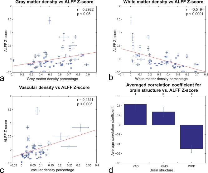
(A–C): Regional analysis (N = 50 regions from atlas template) of relationship between (A) GMD, (B) WMD, and (C) VAD and ALFF Z‐score acorss subjects. (D) Average correlation across regions and subjects between structural density and ALFF Z‐score. The three structures' CCs are statistically significant (P < 0.05). Error bars reflect SEM. [Color figure can be viewed in the online issue, which is available at http://wileyonlinelibrary.com.]

Voxel‐wise relationship between structural density and amplitude of the RS‐fMRI BOLD signal

Figure 3a–c shows the results from the high‐resolution analysis, averaged across all subjects, whereas Figure 3d shows the average correlations across all subjects. In Figure 3a, the correlation between GMD and ALFF Z‐score was 0.6394, higher than its regional counterpart. However, above a GMD of 20%, the ALFF Z‐score stabilized and did not change significantly. The ALFF correlation with VAD was still greater than the one with GMD at this level, and also higher in terms of absolute value than the WMD one. The strong relationship between VAD and RS‐fMRI BOLD was also evident at the single‐subject level (Supporting Information Fig. 4). Figure 3d shows the voxel‐by‐voxel averaged CC between the three structures and the ALFF Z‐score across all subjects. The results confirmed the previous regional approach (Fig. 2) for the VAD and WMD, though not for GMD whose correlations were not significant.

Figure 3.

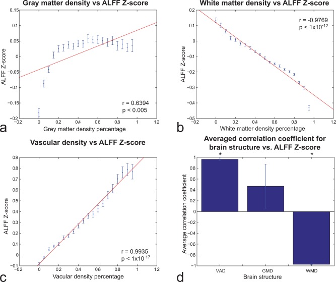
Voxel‐wise analysis of relationship between (A) GMD, (B) WMD, and (C) VAD and ALFF Z‐score acorss subjects. In each subject, GMD, WMD, and VAD values were divided in 20 bins of 5% density each. Each bin contains the average and standard deviation for more than 19 subjects of the ALFF Z‐score for that percentage of structure density. (D) Average of the CC between the three structure densities (GMD, WMD, and VAD) and the ALFF Z‐score. VAD and WMD correlations were statistically significant (P < 0.05). Error bars reflect SEM. [Color figure can be viewed in the online issue, which is available at http://wileyonlinelibrary.com.]

As VAD was the best positively correlated to ALFF Z‐score in both low‐ and high‐resolution approaches, we performed a GLM analysis to study the impact of VAD on the ALFF Z‐score. Figure 4 shows the ALFF Z‐score (Fig. 4a) and the VAD (Fig. 4b), both averaged across the 19 subjects. To proceed to a direct comparison between ALFF Z‐score and VAD on a voxel‐wise basis, a spatial smoothing (FWHM, 6 mm) was first applied to the VAD volume to reduce the mismatch effect of high‐resolution SWI and low‐resolution EPI images, and then subsequently used as a predictor in a GLM. The residuals of this fit (i.e., voxels whose ALFF could not be explained by VAD) are shown in Figure 4c. It is important to note that how a large portion of the voxels originally exhibiting high ALFF values (red/yellow sites, Fig. 4a) is largely suppressed after VAD correction. This effect is particularly strong for voxels within the Cuneus, Culmen, and Frontal Gyrus (Fig. 4d).

Figure 4.

(A) ALFF Z‐Score averaged for more than 19 subjects. (B) VAD averaged for more than 19 subjects (vesselness measure thresholded at 0.01 for every subject). (C) Residual ALFF Z‐score after linear regression of VAD. (D) Panel A minus Panel C, revealing regions where the effect of VAD is most prominent.

Relationship between structural density and amplitude of the T‐fMRI BOLD signal

The correlation between GMD, WMD, and VAD and the % change during a task is shown in Figure 5a–c. The GMD showed no significant correlation with the % change. On the other hand, WMD and VAD show significant negative and positive correlation, respectively, as the RS‐fMRI voxel‐wise analysis showed. Also, in line with the previous regional and voxel approach in RS‐fMRI, T‐fMRI correlations were weakest with GMD compared to VAD and WMD (Fig. 5d).

Figure 5.

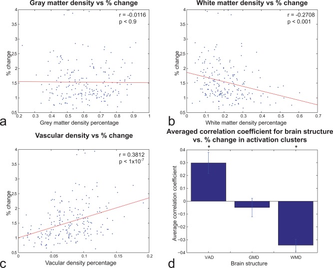
Cluster‐wise (N = 199) analysis of relationship between (A) GMD, (B) WMD, and (C) VAD and T‐fMRI % change during activation for 19 subjects. (D) Average correlation across clusters and subjects between structural density and T‐fMRI % change during activation. VAD and WMD correlations were statistically significant (P < 0.05). Error bars reflect SEM. [Color figure can be viewed in the online issue, which is available at http://wileyonlinelibrary.com.]

A graphic representation of the effect of VAD on the T‐fMRI BOLD signal is shown in Figure 6 in which two activation clusters are overlaid on a segmented SWI image (veins image) from a single participant. One activation cluster showed strong modulation (Fig. 6a–c, 3.98%, red), whereas the other was relatively weak (Fig. 6d–f, 0.9786%, green). When normalizing both signals by their respective VAD, similar modulations were found in both activation clusters.

Figure 6.

Visualization of VAD and its effect on T‐fMRI signal amplitude. (A, B) An activation cluster (red) overlaid on a segmented SWI image from one subject (A: sagittal view. B: axial view). The VAD of this cluster was 25.63%. (C) The average BOLD signal from this activation cluster showed a % change of 3.98%. (D, E) A separate activation cluster (green) from the same subject. The VAD of this cluster was smaller (9.03%) than that of panels A and B. (F) The average BOLD signal from the green activation cluster showed a % change of 0.9786%.

Higher RS ALFF is related to higher % change during task

The relatively strong correlation between VAD–RS‐fMRI and VAD–T‐fMRI suggests that the amplitude of a task‐evoked BOLD signal is related to its amplitude at rest. To investigate this, we compared the ALFF and % change values across activation clusters and subjects (total of 199 clusters). This is shown in Figure 7. The two were significantly correlated, indicating a strong link between the amplitude at rest and the capacity to have pronounced modulation when activated.

Figure 7.

ALFF Z‐score versus the % change for each T‐fMRI activation cluster of each subject. [Color figure can be viewed in the online issue, which is available at http://wileyonlinelibrary.com.]

DISCUSSION

In this study, we used MRI to derive regional measures of GMD and VAD in healthy humans and compared them to BOLD signals obtained during rest (RS‐fMRI) and task (T‐fMRI). For RS‐fMRI, we found a significant positive correlation between regional BOLD amplitude (ALFF) and VAD, whereas correlations with GMD were considerably lower. Similar results were obtained for T‐fMRI. Our findings confirm that the amplitude of the BOLD signal is heavily influenced by the surrounding vasculature, as expected by previous experimental and modeling studies [Bandettini and Wong, 1995, 1997; Menon et al., 1993; Ogawa et al., 1993]. Our study proposes a novel way of suppressing this effect by first computing whole‐brain VAD and then correcting the BOLD response accordingly to better interpret BOLD amplitude in task and resting conditions.

Correlation Between Regional Measures of GMD, WMD, and BOLD Amplitude

Of the three structures investigated in this study, GMD consistently showed the lowest correlation with BOLD amplitude. This was the case during both RS‐fMRI and T‐fMRI. The latter is in line with the study by Oakes et al. [2007] who found that the bulk of fMRI activation clusters were unaffected when using GMD as a covariate, suggesting that the fMRI activations may not solely be driven by GM differences. This is also supported by two recent studies which measured brain structure and fMRI activity before and after extensive training of a visuospatial task. In both cases, they found that regional changes in GMD [Thomas et al., 2009] and GM thickness [Haier et al., 2009] did not match the changes in fMRI, indicating that a structural change in one brain area does not necessarily result in functional change in the same location. Concerning RS‐fMRI signals, Wang et al. [2011] measured ALFF in healthy controls and Alzheimer's disease patients. They found that while taking GM volume as covariate, the ALFF results were approximately consistent with those without GM correction, implying that the differences observed with ALFF could not be explained by regional GM atrophy. Our findings therefore add to the growing body of evidence, suggesting that regional variations in GMD (as derived from VBM) are not strong predictors of the BOLD response amplitude. The reason behind this is unclear. On the one hand, the underlying cytoarchitecture giving rise to VBM–GMD measurements may not directly relate to the amplitude of hemodynamic activity measured with fMRI. However, it is difficult to accurately interpret the meaning of GMD measures as they should not be confused with cell‐packing density measured cytoarchitectonically [Mechelli et al., 2005].

Concerning the WM, several studies have found that that the amplitude of the BOLD signal is approximately 60–80% greater in GM than in WM [Biswal et al., 1995; Cordes et al., 2001; Yan et al., 2009; Zang et al., 2007; Zou et al., 2008; Zuo et al., 2010]. We observed a negative correlation between ALFF and WMD, as well as for T‐fMRI amplitude. These findings are well in line with the studies of Polimeni et al. [2010] and Zuo et al. [2010], respectively. However, as this structure is often discarded in BOLD fMRI studies, it is left for further study.

Correlation Between Regional Measures of VAD and BOLD Amplitude

Compared to GMD, we found that regional variations in VAD were significantly better correlated to RS‐fMRI and T‐fMRI. It is well established that BOLD signals arise mainly from changes in oxygenation in venules and veins lying relatively close to the site of increased neuronal activity [Song et al., 1996]. We demonstrated that the density of such venules has a significant impact on the observed amplitude of the BOLD signal. This is supported by the modeling study by Turner [2002], who found that neural‐induced changes in oxygenation become diluted at greater distances along the draining vein. Therefore, voxels embedded in an area rich in vasculature will have, on average, a shorter distance to the nearest vein. In these voxels, the dilution effect would be less and thus reflect stronger BOLD amplitude. This is in line with the seminal study of Kim et al. [1994], who observed that the temporal variance of the BOLD signal during rest was greater within large veins than within cortex. This may be caused by mechanical factors such as vascular vasomotion and cerebral microcirculation [Mayhew et al., 1996; Mitra et al., 1997; Razavi et al., 2008; Shmueli et al., 2007], which oscillate at a frequency of approximately 0.1 Hz. These oscillations are most likely prominent in large veins and may contribute to the ALFF measure (e.g., via partial volume effects) by increasing the 0.1 Hz amplitude in the power spectrum of voxels within a heavily vascularized area. We also observed a significant correlation between VAD and T‐fMRI though the source of this relationship is less clear. Given the tight link between baseline CBV_venous and task‐evoked BOLD amplitude [Moon et al., 2013; Yu et al., 2012; Zhao et al., 2006], cortical areas with different CBV_venous (and consequently, different VADs) will have different stimulus‐evoked BOLD responses even if oxygenation level changes are similar between them [Kim and Ogawa, 2012]. This would also explain the strong correlation we observed between ALFF and % change (Fig. 7). However, in separate areas with similar CBV_venous, the one with a stronger stimulus‐evoked CBF response will induce higher oxygenation and consequently, a higher BOLD response. Owing to the limited field strength used in our study (1.5T), the vessels segmented by our algorithm are most likely to be the larger vessels with high CBF (according to Poiseuille's equation of a Newtonian fluid). It would be very interesting to repeat our study at higher field strength and investigate whether our algorithm can detect areas densely packed with smaller venules (i.e., areas with high VAD though low CBF), and how BOLD amplitude is modulated in these areas. Taken together, notwithstanding its biological underpinnings, the tight link between VAD and T‐fMRI suggests that certain brain areas are inherently structured to elicit larger BOLD responses.

Implications

Regional variations in VAD carry important implications on the interpretation of neural activity derived from fMRI (neurovascular coupling). First, we found that using VAD as a covariate in fMRI analysis helps remove false positives in RS activity (i.e., voxels with ALFF values greater than a given threshold value). Although not explicitly studied here, segmented SWI images (VAD) may also aid in suppressing downstream sites with large venous contribution and thus increase the spatial specificity of BOLD activation maps [Barth and Norris, 2007; Menon, 2002; Rowe and Logan, 2004]. Normalizing BOLD activity by vascular structure may be particularly important for clinical fMRI studies where there are a growing number of studies reporting on differences in RS amplitude between healthy controls and patients with various neurological disorders [Chen et al., 2009; Jiao et al., 2011; Wang et al., 2011; Xi et al., 2012; Zang et al., 2007]. Without correcting for vascular structure, our findings suggest that, particularly in patients with neurovascular disorders, a diminished BOLD response should not be simply interpreted as a decrease in neural activity, but could reflect damage or a change in vascular architecture. Second, the measures of VAD may also help reconcile regional discrepancies in neurovascular coupling. For instance, in area MT, Rees et al. [2000] found that a 1% change in the fMRI signal corresponded to a change in average firing rate of nine spikes/second per neuron, whereas in area V1, Heeger et al. [2000] found 0.4 spikes/second per neuron for each 1% change in the fMRI signal. Although converging evidence points to the local field potential (LFP) as being a better correlate of BOLD than spiking activity [Logothetis, 2008], the relationship between LFP and BOLD is also region dependent [Conner et al., 2011; Devonshire et al., 2012; Sloan et al., 2010]. The reason how regional variations in the relationship between neural and hemodynamic signals relate to VAD is left for further study. Taken together, our findings indicate that while variations in fMRI activity are neural in nature [Magri et al., 2012; Pan et al., 2011; Schölvinck et al., 2010], brain areas with high VAD may cause the BOLD response to appear amplified relative to others.

CONCLUSIONS

Our study adds to the growing body of the literature aimed at accounting for hemodynamic variability over space [Ances et al., 2008; Bandettini and Wong, 1995; Chiarelli et al., 2007; Hoge et al., 1999; Kannurpatti et al., 2012; Kida et al., 2007; Menon et al., 1993; Ogawa et al., 1993; Thomason et al., 2007]. As SWI sequences are available on most MR scanners, we would recommend—as stated by Haacke and Ye [2012]—that all fMRI experiments that collect T1‐weighted images for anatomical information also collect a high‐resolution SWI scan to monitor the venous vasculature in the activated regions of interest or across different subject groups. Using the measures of VAD as a covariate in RS fMRI studies can help to more precisely detect the neural portion of the BOLD signal, and thus provide improved interpretation of brain function in humans. The procedure for vesselness computation and VAD modeling of the fMRI will soon be available as a Statistical Parametric Mapping (SPM) plugin (http://pages.usherbrooke.ca/vesselsegmentation/).

Supporting information

Supporting Information

REFERENCES

- Ances BM, Leontiev O, Perthen JE, Liang C, Lansing AE, Buxton RB (2008): Regional differences in the coupling of cerebral blood flow and oxygen metabolism changes in response to activation: Implications for BOLD‐fMRI. NeuroImage 39:1510–1521. [DOI] [PMC free article] [PubMed] [Google Scholar]
- Attwell D, Iadecola C (2002): The neural basis of functional brain imaging signals. Trends Neurosci 25:621–625. [DOI] [PubMed] [Google Scholar]
- Attwell D, Buchan AM, Charpak S, Lauritzen M, MacVicar BA, Newman EA (2010): Glial and neuronal control of brain blood flow. Nature 468:232–243. [DOI] [PMC free article] [PubMed] [Google Scholar]
- Bandettini PA (2012): Functional MRI: A confluence of fortunate circumstances. NeuroImage 1–9. [DOI] [PMC free article] [PubMed] [Google Scholar]
- Bandettini PA, Wong EC (1995): Effects of biophysical and physiologic parameters on brain activation‐induced R2* and R2 changes: Simulations using a deterministic diffusion model. Int J Imaging Syst Technol 6:133–152. [Google Scholar]
- Bandettini PA, Wong EC (1997): A hypercapnia‐based normalization method for improved spatial localization of human brain activation with fMRI. NMR Biomed 10:197–203. [DOI] [PubMed] [Google Scholar]
- Bandettini PA, Jesmanowicz A, Wong EC, Hyde JS (1993): Processing strategies for time‐course data sets in functional MRI of the human brain. Magn Reson Med 30:161–173. [DOI] [PubMed] [Google Scholar]
- Barth M, Norris DG (2007): Very high‐resolution three‐dimensional functional MRI of the human visual cortex with elimination of large venous vessels. NMR Biomed 20:477–484. [DOI] [PubMed] [Google Scholar]
- Bianciardi M, Fukunaga M, Van Gelderen P, De Zwart JA, Duyn JH (2011): Negative BOLD‐fMRI signals in large cerebral veins. J Cereb Blood Flow Metab 31:401–412. [DOI] [PMC free article] [PubMed] [Google Scholar]
- Biswal B, Yetkin FZ, Haughton VM, Hyde JS (1995): Functional connectivity in the motor cortex of resting human brain using echo‐planar MRI. Magn Reson Med 34:537–541. [DOI] [PubMed] [Google Scholar]
- Brevard ME, Duong TQ, King JA, Ferris CF (2003): Changes in MRI signal intensity during hypercapnic challenge under conscious and anesthetized conditions. Magn Reson Imaging 21:995–1001. [DOI] [PMC free article] [PubMed] [Google Scholar]
- Bright MG, Bulte DP, Jezzard P, Duyn JH (2009): Characterization of regional heterogeneity in cerebrovascular reactivity dynamics using novel hypocapnia task and BOLD fMRI. NeuroImage 48:166–175. [DOI] [PMC free article] [PubMed] [Google Scholar]
- Buxton RB, Uludağ K, Dubowitz DJ, Liu TT (2004): Modeling the hemodynamic response to brain activation. NeuroImage 23:S220–S233. [DOI] [PubMed] [Google Scholar]
- Casciaro S, Bianco R, Distante A (2008): Quantification of venous blood signal contribution to BOLD functional activation in the auditory cortex at 3T. Magn Reson Imaging 26:1221–1231. [DOI] [PubMed] [Google Scholar]
- Chen Q, Lui S, Zhang S, Tang H, Wang J, Huang X, Gong Q, Zhou D, Shang H (2009): Amplitude of low frequency fluctuation of BOLD signal and resting‐state functional connectivity analysis of brains of Parkinson's disease. Proceedings of the 17th Scientific Meeting, International Society for Magnetic Resonance in Medicine 17:735. [Google Scholar]
- Chiarelli PA, Bulte DP, Piechnik S, Jezzard P (2007): Sources of systematic bias in hypercapnia‐calibrated functional MRI estimation of oxygen metabolism. NeuroImage 34:35–43. [DOI] [PubMed] [Google Scholar]
- Conner CR, Ellmore TM, Pieters TA, Disano MA, Tandon N (2011): Variability of the relationship between electrophysiology and BOLD‐fMRI across cortical regions in humans. J Neurosci 31:12855–12865. [DOI] [PMC free article] [PubMed] [Google Scholar]
- Cordes D, Haughton VM, Arfanakis K, Carew JD, Turski PA, Moritz CH, Quigley MA, Meyerand ME (2001): Frequencies contributing to functional connectivity in the cerebral cortex in “resting‐state” data. AJNR Am J Neuroradiol 22:1326–1333. [PMC free article] [PubMed] [Google Scholar]
- Cox RW (1996): AFNI: Software for analysis and visualization of functional magnetic resonance neuroimages. Comp Biomed Res 29:162–173. [DOI] [PubMed] [Google Scholar]
- Davis TL, Kwong KK, Weisskoff RM, Rosen BR (1998): Calibrated functional MRI: Mapping the dynamics of oxidative metabolism. Proc Natl Acad Sci USA 95:1834–1839. [DOI] [PMC free article] [PubMed] [Google Scholar]
- Descoteaux M, Collins L, Siddiqi K (2004): Geometric flows for segmenting vasculature in MRI: Theory and validation. Medical Image Computing and ComputerAssisted Intervention Miccai 2004 Pt 1 Proceedings 3216, 500–507. [Google Scholar]
- Descoteaux M, Collins DL, Siddiqi K (2008): A geometric flow for segmenting vasculature in proton‐density weighted MRI. Med Image Anal 12:497–513. [DOI] [PubMed] [Google Scholar]
- Devonshire IM, Papadakis NG, Port M, Berwick J, Kennerley AJ, Mayhew JEW, Overton PG (2012): Neurovascular coupling is brain region‐dependent. NeuroImage 59:1997–2006. [DOI] [PubMed] [Google Scholar]
- Duvernoy HM, Delon S, Vannson JL (1981): Cortical blood vessels of the human brain. Brain Res Bull 7:519–579. [DOI] [PubMed] [Google Scholar]
- Ekstrom A (2010): How and when the fMRI BOLD signal relates to underlying neural activity: The danger in dissociation. Brain Res Rev 62:233–244. [DOI] [PMC free article] [PubMed] [Google Scholar]
- Fox MD, Raichle ME (2007): Spontaneous fluctuations in brain activity observed with functional magnetic resonance imaging. Nat Rev Neurosci 8:700–711. [DOI] [PubMed] [Google Scholar]
- Fox PT, Raichle ME (1986): Focal physiological uncoupling of cerebral blood flow and oxidative metabolism during somatosensory stimulation in human subjects. Proc Natl Acad Sci USA 83:1140–1144. [DOI] [PMC free article] [PubMed] [Google Scholar]
- Frangi AF, Niessen WJ, Vincken KL, Viergever MA (1998): Multiscale vessel enhancement filtering 1 Introduction 2 Method. Computer 1496:130–137. [Google Scholar]
- Gusnard DA, Raichle ME (2001): Searching for a baseline: Functional imaging and the resting human brain. Nat Rev Neurosci 2:685–694. [DOI] [PubMed] [Google Scholar]
- Haacke EM, Xu Y, Cheng Y‐CN, Reichenbach JR (2006): Susceptibility weighted imaging (SWI). Zeitschrift medizinische Physik 52:612–618. [Google Scholar]
- Haacke EM, Ye Y (2012): The role of susceptibility weighted imaging in functional MRI. NeuroImage 62:923–929. [DOI] [PubMed] [Google Scholar]
- Haier RJ, Karama S, Leyba L, Jung RE (2009): MRI assessment of cortical thickness and functional activity changes in adolescent girls following three months of practice on a visual‐spatial task. Biomed Chromatogr Res Notes 2:174. [DOI] [PMC free article] [PubMed] [Google Scholar]
- Hall DA, Gonçalves MS, Smith S, Jezzard P, Haggard MP, Kornak J (2002): A method for determining venous contribution to BOLD contrast sensory activation. Magn Res Imaging 20:695–706. [DOI] [PubMed] [Google Scholar]
- Handwerker DA, Gonzalez‐Castillo J, D'Esposito M, Bandettini PA (2012): The continuing challenge of understanding and modeling hemodynamic variation in fMRI. NeuroImage 62:1017–1023. [DOI] [PMC free article] [PubMed] [Google Scholar]
- Harrison RV, Harel N, Panesar J, Mount RJ (2002): Blood capillary distribution correlates with hemodynamic‐based functional imaging in cerebral cortex. Cereb Cortex 12:225–233. [DOI] [PubMed] [Google Scholar]
- Heeger DJ, Huk AC, Geisler WS, Albrecht DG (2000): Spikes versus BOLD: What does neuroimaging tell us about neuronal activity? Nat Neurosci 3:631–633. [DOI] [PubMed] [Google Scholar]
- Hoge RD, Atkinson J, Gill B, Crelier GR, Marrett S, Pike GB (1999): Investigation of BOLD signal dependence on cerebral blood flow and oxygen consumption: The deoxyhemoglobin dilution model. Magn Reson Med 42:849–863. [DOI] [PubMed] [Google Scholar]
- Hoogenraad FG, Hofman MB, Pouwels PJ, Reichenbach JR, Rombouts SA, Haacke EM (1999): Sub‐millimeter fMRI at 1.5 Tesla: Correlation of high resolution with low resolution measurements. J Magn Reson Imaging 9:475–482. [DOI] [PubMed] [Google Scholar]
- Jiao Q, Lu G, Zhang Z, Zhong Y, Wang Z, Guo Y, Li K, Ding M, Liu Y (2011): Granger causal influence predicts BOLD activity levels in the default mode network. Hum Brain Map 32:154–161. [DOI] [PMC free article] [PubMed] [Google Scholar]
- Jochimsen TH, Ivanov D, Ott DVM, Heinke W, Turner R, Möller HE, Reichenbach JR (2010): Whole‐brain mapping of venous vessel size in humans using the hypercapnia‐induced BOLD effect. NeuroImage 51:765–774. [DOI] [PubMed] [Google Scholar]
- Kannurpatti SS, Rypma B, Biswal BB (2012): Prediction of task‐related BOLD fMRI with amplitude signatures of resting‐state fMRI. Front Syst Neurosci 6:7. [DOI] [PMC free article] [PubMed] [Google Scholar]
- Kida I, Rothman DL, Hyder F (2007): Dynamics of changes in blood flow, volume, and oxygenation: Implications for dynamic functional magnetic resonance imaging calibration. J Cereb Blood Flow Metab 27:690–696. [DOI] [PMC free article] [PubMed] [Google Scholar]
- Kim S‐G, Ogawa S (2012): Biophysical and physiological origins of blood oxygenation level‐dependent fMRI signals. J Cereb Blood Flow Metab 32:1–19. [DOI] [PMC free article] [PubMed] [Google Scholar]
- Kim SG, Hendrich K, Hu X, Merkle H, Uğurbil K (1994): Potential pitfalls of functional MRI using conventional gradient‐recalled echo techniques. NMR Biomed 7:69–74. [DOI] [PubMed] [Google Scholar]
- Leontiev O, Buxton RB (2007): Reproducibility of BOLD, perfusion, and CMRO2 measurements with calibrated‐BOLD fMRI. NeuroImage 35:175–184. [DOI] [PMC free article] [PubMed] [Google Scholar]
- Logothetis NK (2002): The neural basis of the blood‐oxygen‐level‐dependent functional magnetic resonance imaging signal. Philos Trans R Soc Lond B Biol Sci 357:1003–1037. [DOI] [PMC free article] [PubMed] [Google Scholar]
- Logothetis NK (2008): What we can do and what we cannot do with fMRI. Nature 453:869–878. [DOI] [PubMed] [Google Scholar]
- Magri C, Schridde U, Murayama Y, Panzeri S, Logothetis NK (2012): The amplitude and timing of the BOLD signal reflects the relationship between local field potential power at different frequencies. J Neurosci 32:1395–1407. [DOI] [PMC free article] [PubMed] [Google Scholar]
- Mayhew JE, Askew S, Zheng Y, Porrill J, Westby GW, Redgrave P, Rector DM, Harper RM (1996): Cerebral vasomotion: A 0.1‐Hz oscillation in reflected light imaging of neural activity. NeuroImage 4:183–193. [DOI] [PubMed] [Google Scholar]
- Mechelli A, Friston KJ, Frackowiak RS, Price CJ (2005): Structural covariance in the human cortex. J Neurosci 25:8303–8310. [DOI] [PMC free article] [PubMed] [Google Scholar]
- Menon RS (2002): Postacquisition suppression of large‐vessel BOLD signals in high‐resolution fMRI. Magn Reson Med 47:1–9. [DOI] [PubMed] [Google Scholar]
- Menon RS, Ogawa S, Tank DW, Uğurbil K (1993): Tesla gradient recalled echo characteristics of photic stimulation‐induced signal changes in the human primary visual cortex. Magn Reson Med 30:380–386. [DOI] [PubMed] [Google Scholar]
- Mitra PP, Ogawa S, Hu X, Uğurbil K (1997): The nature of spatiotemporal changes in cerebral hemodynamics as manifested in functional magnetic resonance imaging. Magn Reson Med 37:511–518. [DOI] [PubMed] [Google Scholar]
- Moon CH, Fukuda M, Kim S‐G (2013): Spatiotemporal characteristics and vacular sources of neural‐specific and ‐nonspecific fMRI signals at submillimeter columnar resolution. NeuroImage 64:91–103. [DOI] [PMC free article] [PubMed] [Google Scholar]
- Nair DG (2005): About being BOLD. Brain Res Brain Res Rev 50:229–243. [DOI] [PubMed] [Google Scholar]
- Oakes TR, Fox AS, Johnstone T, Chung MK, Kalin N, Davidson RJ (2007): Integrating VBM into the General Linear Model with voxelwise anatomical covariates. NeuroImage 34:500–508. [DOI] [PMC free article] [PubMed] [Google Scholar]
- Ogawa S, Menon RS, Tank DW, Kim SG, Merkle H, Ellermann JM, Ugurbil K (1993): Functional brain mapping by blood oxygenation level‐dependent contrast magnetic resonance imaging. Biophys J 64:803–812. [DOI] [PMC free article] [PubMed] [Google Scholar]
- Pan W‐J, Thompson G, Magnuson M, Majeed W, Jaeger D, Kelholz S (2011): Broadband local field potentials correlate with spontaneous fluctuations in functional magnetic resonance imaging signals in the rat somatosensory cortex under isoflurane anesthesia. Brain Connect 1:119–131. [DOI] [PMC free article] [PubMed] [Google Scholar]
- Polimeni JR, Fischl B, Greve DN, Wald LL (2010): Laminar analysis of 7T BOLD using an imposed spatial activation pattern in human V1. NeuroImage 52:1334–1346. [DOI] [PMC free article] [PubMed] [Google Scholar]
- Qi R, Zhang L, Wu S, Zhong J, Zhang Z, Zhong Y, Ni L, Zhang Z, Li K, Jiao Q, Wu X, Fan X, Liu Y, Lu G (2012): Altered resting‐state brain activity at functional MR imaging during the progression of hepatic encephalopathy. Radiology 264:187–195. [DOI] [PubMed] [Google Scholar]
- Razavi M, Eaton B, Paradiso S, Mina M, Hudetz AG, Bolinger L (2008): Source of low‐frequency fluctuations in functional MRI signal. J Magn Reson Imaging 27:891–897. [DOI] [PubMed] [Google Scholar]
- Rees G, Friston K, Koch C (2000): A direct quantitative relationship between the functional properties of human and macaque V5. Nat Neurosci 3:716–723. [DOI] [PubMed] [Google Scholar]
- Roland PE, Eriksson L, Stone‐Elander S, Widen L (1987): Does mental activity change the oxidative metabolism of the brain? J Neurosci 7:2373–2389. [PMC free article] [PubMed] [Google Scholar]
- Rowe DB, Logan BR (2004): A complex way to compute fMRI activation. NeuroImage 23:1078–1092. [DOI] [PubMed] [Google Scholar]
- Schölvinck ML, Maier A, Ye FQ, Duyn JH, Leopold DA (2010): Neural basis of global resting‐state fMRI activity. Proc Natl Acad Sci USA 107:10238–10243. [DOI] [PMC free article] [PubMed] [Google Scholar]
- Seiyama A, Seki J, Tanabe HC, Sase I, Takatsuki A, Miyauchi S, Eda H, Hayashi S, Imaruoka T, Iwakura T, Yanagida T (2004): Circulatory basis of fMRI signals: Relationship between changes in the hemodynamic parameters and BOLD signal intensity. NeuroImage 21:1204–1214. [DOI] [PubMed] [Google Scholar]
- Shmueli K, Van Gelderen P, De Zwart JA, Horovitz SG, Fukunaga M, Jansma JM, Duyn JH (2007): Low‐frequency fluctuations in the cardiac rate as a source of variance in the resting‐state fMRI BOLD signal. NeuroImage 38:306–320. [DOI] [PMC free article] [PubMed] [Google Scholar]
- Sloan HL, Austin VC, Blamire AM, Schnupp JWH, Lowe AS, Allers KA, Matthews PM, Sibson NR (2010): Regional differences in neurovascular coupling in rat brain as determined by fMRI and electrophysiology. NeuroImage 53:399–411. [DOI] [PubMed] [Google Scholar]
- Smith SM, Jenkinson M, Woolrich MW, Beckmann CF, Behrens TEJ, Johansen‐Berg H, Bannister PR, De Luca M, Drobnjak I, Flitney DE, Niazy RK, Saunders J, Vickers J, Zhang Y, De Stefano N, Brady JM, Matthews PM (2004): Advances in functional and structural MR image analysis and implementation as FSL. NeuroImage 23:S208–S219. [DOI] [PubMed] [Google Scholar]
- Song AW, Wong EC, Tan SG, Hyde JS (1996): Diffusion weighted fMRI at 1.5T. Magn Reson Med 35:155–158. [DOI] [PubMed] [Google Scholar]
- Thomas AG, Marrett S, Saad ZS, Ruff DA, Martin A, Bandettini PA (2009): Functional but not structural changes associated with learning: An exploration of longitudinal voxel‐based morphometry (VBM). NeuroImage 48:117–125. [DOI] [PMC free article] [PubMed] [Google Scholar]
- Thomason ME, Foland LC, Glover GH (2007): Calibration of BOLD fMRI using breath holding reduces group variance during a cognitive task. Hum Brain Map 28:59–68. [DOI] [PMC free article] [PubMed] [Google Scholar]
- Turner R (2002): How much cortex can a vein drain? Downstream dilution of activation‐related cerebral blood oxygenation changes. NeuroImage 16:1062–1067. [DOI] [PubMed] [Google Scholar]
- Uludağ K, Müller‐Bierl B, Uğurbil K (2009): An integrative model for neuronal activity‐induced signal changes for gradient and spin echo functional imaging. NeuroImage 48:150–165. [DOI] [PubMed] [Google Scholar]
- Wang Z, Jia X, Liang P, Qi Z, Yang Y, Zhou W, Li K (2011): Changes in thalamus connectivity in mild cognitive impairment: Evidence from resting state fMRI. Eur J Radiol 19:3575. [DOI] [PubMed] [Google Scholar]
- Wang Z, Yan C, Zhao C, Qi Z, Zhou W, Lu J, He Y, Li K (2011): Spatial patterns of intrinsic brain activity in mild cognitive impairment and Alzheimer's disease: A resting‐state functional MRI study. Hum Brain Map 32:1720–1740. [DOI] [PMC free article] [PubMed] [Google Scholar]
- Weber B, Keller AL, Reichold J, Logothetis NK (2008): The microvascular system of the striate and extrastriate visual cortex of the macaque. Cereb Cortex 18:2318–2330. [DOI] [PubMed] [Google Scholar]
- Woolrich MW, Jbabdi S, Patenaude B, Chappell M, Makni S, Behrens T, Beckmann C, Jenkinson M, Smith SM (2009): Bayesian analysis of neuroimaging data in FSL. NeuroImage 45:S173–S186. [DOI] [PubMed] [Google Scholar]
- Xi Q, Zhao X‐H, Wang P‐J, Guo Q‐H, Yan C‐G, He Y (2012): Functional MRI study of mild Alzheimer's disease using amplitude of low frequency fluctuation analysis. Chin Med J Engl 125:858–862. [PubMed] [Google Scholar]
- Yan L, Zhuo Y, Ye Y, Xie SX, An J, Aguirre GK, Wang J (2009): Physiological origin of low‐frequency drift in blood oxygen level dependent (BOLD) functional magnetic resonance imaging (fMRI). Magn Reson Med 61:819–827. [DOI] [PubMed] [Google Scholar]
- Yu X, Glen D, Wang S, Dodd S, Hirano Y, Saad Z, Reynolds R, Silva AC, Koretsky AP (2012): Direct imaging of macrovascular and microvascular contributions to BOLD fMRI in layers IV‐V of the rat whisker‐barrel cortex. NeuroImage 59:1451–1460. [DOI] [PMC free article] [PubMed] [Google Scholar]
- Zang Y‐F, He Y, Zhu C‐Z, Cao Q‐J, Sui M‐Q, Liang M, Tian L‐X, Jiang T‐Z, Wang Y‐F (2007): Altered baseline brain activity in children with ADHD revealed by resting‐state functional MRI. Brain Dev 29:83–91. [DOI] [PubMed] [Google Scholar]
- Zhao F, Wang P, Hendrich K, Ugurbil K, Kim S‐G (2006) Cortical layer‐dependent BOLD and CBV responses measured by spin‐echo and gradient‐echo fMRI: Insights into hemodynamic regulation. NeuroImage 30:1149–1160. [DOI] [PubMed] [Google Scholar]
- Zou Q‐H, Zhu C‐Z, Yang Y, Zuo X‐N, Long X‐Y, Cao Q‐J, Wang Y‐F, Zang Y‐F (2008): An improved approach to detection of amplitude of low‐frequency fluctuation (ALFF) for resting‐state fMRI: Fractional ALFF. J Neurosci Methods 172:137–141. [DOI] [PMC free article] [PubMed] [Google Scholar]
- Zuo X‐N, Di Martino A, Kelly C, Shehzad ZE, Gee DG, Klein DF, Castellanos FX, Biswal BB, Milham MP (2010): The oscillating brain: Complex and reliable. NeuroImage 49:1432–1445. [DOI] [PMC free article] [PubMed] [Google Scholar]
Associated Data
This section collects any data citations, data availability statements, or supplementary materials included in this article.
Supplementary Materials