

Abstract
Accurate tissue classification is a crucial prerequisite to MRI morphometry. Automated methods based on intensity histograms constructed from the entire volume are challenged by regional intensity variations due to local radiofrequency artifacts as well as disparities in tissue composition, laminar architecture and folding patterns. Current work proposes a novel anatomy‐driven method in which parcels conforming cortical folding were regionally extracted from the brain. Each parcel is subsequently classified using nonparametric mean shift clustering. Evaluation was carried out on manually labeled images from two datasets acquired at 3.0 Tesla (n = 15) and 1.5 Tesla (n = 20). In both datasets, we observed high tissue classification accuracy of the proposed method (Dice index >97.6% at 3.0 Tesla, and >89.2% at 1.5 Tesla). Moreover, our method consistently outperformed state‐of‐the‐art classification routines available in SPM8 and FSL‐FAST, as well as a recently proposed local classifier that partitions the brain into cubes. Contour‐based analyses localized more accurate white matter–gray matter (GM) interface classification of the proposed framework compared to the other algorithms, particularly in central and occipital cortices that generally display bright GM due to their highly degree of myelination. Excellent accuracy was maintained, even in the absence of correction for intensity inhomogeneity. The presented anatomy‐driven local classification algorithm may significantly improve cortical boundary definition, with possible benefits for morphometric inference and biomarker discovery. Hum Brain Mapp 36:3563–3574, 2015. © 2015 Wiley Periodicals, Inc.
Keywords: MRI classification, segmentation, local histogram, myelination, neocortex, inhomogeneity
INTRODUCTION
Accurate MRI tissue classification is paramount to state‐of‐the‐art brain morphometry such as voxel‐based morphometry, quantification of cortical thickness, and analysis of cortical folding and complexity. Commonly, classification algorithms establish decision boundaries on MR intensities to identify gray matter (GM), white matter (WM), cerebrospinal fluid (CSF), and sometimes mixtures of them. Most classifiers analyze global intensity histograms constructed from the entire volume [Ashburner and Friston, 2005; Collins et al., 1999; Fischl et al., 2004; Zhang et al., 2001]. A global approach might, however, be challenged by local intensity inhomogeneity due to radiofrequency artifacts occurring during image acquisition, an effect amplified at higher field strengths [Boyes et al., 2008]. Since classification performance relies heavily on correction of this artifact [Sled et al., 1998; Tustison et al., 2010; Zheng et al., 2009], MRI processing packages, such as FSL [Jenkinson et al., 2012; Zhang et al., 2001] and SPM [Ashburner and Friston, 2005], routinely incorporate inhomogeneity correction methods.
Regional variations in cortical lamination, myelination [Geyer et al., 2011; Glasser and Van Essen, 2011; Sereno et al., 2013], and folding patterns [Sanchez‐Panchuelo et al., 2014] may also cause local intensity inhomogeneity. On T1‐weighted MRI, the most widely used contrast for brain morphometry, highly myelinated central, and occipital cortices display intensity characteristics closer to the WM than to the GM of less myelinated cortices. Consequently, current classification algorithms generally underestimate GM in these regions, resulting in artificially thin cortex. In addition to normal biological variability, pathology‐derived anomalies such as neuronal loss [Bernhardt et al., 2010; Lerch et al., 2005], gliosis [Tam et al., 2011], and cytological alterations [Colliot et al., 2006; Hong et al., 2014; Lerch et al., 2005] may modify image intensity, challenging subsequent tissue classification.
Previously, techniques that used voxel‐wise local Gaussian mixtures [Grabowski et al., 2000; Joshi et al., 1999] or an interpolation of partially overlapping models [Grabowski et al., 2000] have attempted to segment brain tissues under regional intensity variations. More recent approaches have combined Gaussian mixtures and cooperative local Markov random fields [Richard et al., 2007; Scherrer et al., 2009] to ensure smooth transitions; others have used combinations of multicontext fuzzy C‐means (FCM) with information fusion [Zhu and Jiang, 2003], or local FCM models with nonlocal means [Caldairou et al., 2011]. Although these local histogram‐based approaches performed better on MRIs with strong intensity inhomogeneity due to radiofrequency artifacts, they may not cope with intensity varying along the cortical folding, the direction of which is difficult for them to model.
The current work proposes a novel MRI classification method that varies decision boundaries locally according to brain parcels shaped with respect to cortical anatomy. Classification performance was evaluated against manual labels from two independent datasets (1.5 Tesla, n = 20; and 3.0 Tesla, n = 15). We furthermore compared our algorithm to widely used state‐of‐the‐art tissue classifiers, namely SPM8 [Ashburner and Friston, 2005] and FSL‐FAST [Zhang et al., 2001], as well as a recently developed method that used a local classification algorithm based on a cubic (nonanatomical) partitioning [Caldairou et al., 2011].
MATERIALS AND METHODS
Processing steps are illustrated in Figure 1. The algorithm mainly included two stages: (A) Automatic brain parcellation: We first identifed cortical sampling points lying close to a preliminary CSF skeleton, following cortical folding patterns. We generated local parcels around the sampling points and obtained intensity histograms. Overlapping was allowed between neighboring parcels; (B) Tissue classification: Within each parcel, nonparametric clustering was then used to formulate decision boundaries that were subsequently continuously interpolated to all brain voxels, resulting in the final classification.
Figure 1.
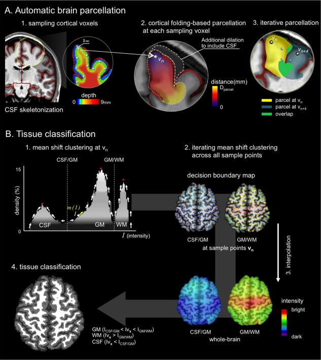
Flowchart of the proposed algorithm. (A) Guided by a preliminary CSF skeleton (red), sampling points in the cortex were identified at a depth of 2 mm. Euclidian distance maps respecting cortical folding were computed and binarized at D parcel mm. Each parcel underwent a selective morphological dilation adding likely CSF candidates. (B) In each parcel, nonparametric mean shift clustering identified peaks of the intensity histogram, assigning decision boundaries to the sampling points. Final whole‐brain classification was obtained after interpolating decision boundaries from sampling voxels to individual brain voxels, using an inverse distance weighting. [Color figure can be viewed in the online issue, which is available at http://wileyonlinelibrary.com.]
Automatic Brain Parcellation
T1‐weighted MRI were skull‐stripped using BEaST, a brain extraction algorithm based on nonlocal means [Eskildsen et al., 2012]. We generated a preliminary CSF skeleton (which was refined in a later step) based on partial volume probabilities of CSF (Fig. 1A‐1) [Kim et al., 2005; Tohka et al., 2004]. In brief, we estimated voxel‐wise CSF partial volume densities using a maximum a prior approach described in [Kim et al., 2005; Tohka et al., 2004]. The CSF partial volume was then binarized by setting any voxel containing CSF to 1 and all others to 0. We then skeletonized this volume using a 2‐subfield connectivity‐preserving medial surface skeletonization algorithm [Ma, IEEE Trans. Pattern. Anal. 2002]. Within the brain mask, we identified sampling points as voxels (Let vn be a sampling voxel, n be a vector in the Cartesian coordinates and N be the number of the total sampling voxels) at the distance of D CSF = 2 mm from this skeleton using the Chamfer distance transform (Fig. 1A‐1). This value was heuristically chosen to approximate half the average cortical thickness. We ignored sampling points around the ventricles, as our aim was to classify cortical GM and WM. Creating parcels at every sampling points and subsequent tissue classifications within each parcel may cause extensive computational time. To accelerate computations, the sampling points were, thus, downsampled at every distance Rmm from {0,0,0} in x,y,z directions in the MR image space as in a multiresolution approach [Eskildsen et al., 2012]. The R is a Euclidean distance and was determined empirically.
From a given sampling point, we performed the Euclidean distance transform to all brain voxels, anatomically constrained by the CSF skeleton (Fig. 1A‐2). This transform allowed propagations of distance map from the sampling point to all other voxels in an iterative fashion. At each iteration, we removed the distance propagation to any skeleton voxel to prevent the distance from propagating from one cortex to its neighboring cortices. Thresholding this distance map at D parcel (chosen empirically, see below) generated a cortical parcel referenced to the sampling point. Because the current parcel includes only GM and WM by design, we further extended the parcel to include CSF voxels through a selective morphological dilation (3 mm, chosen to best balance between tissue types) that adds voxels darker than the lowest intensity of the initial parcel (henceforth, likely CSF candidates). These parcels then contained candidates for all tissue types. We heuristically dilated by 3 mm. The parcellation was iterated for all the sampling points (Fig. 1A‐3).
Tissue Classification
For each parcel created from a given sampling voxel v n D parcel | v n, we built an intensity histogram H | v n to identify GM, WM, and CSF (Fig. 1B‐1). Because intensity inhomogeneity, partial volume, and background noise may generate a skewed histogram, we used nonparametric mean‐shift clustering to robustly identify the peaks in the histrogram [Comaniciu and Meer, 2002]. At a given intensity I on the histogram H | v n, the mean shift m was defined as:
| (1) |
Kσ(·) is a histogram density estimator with the Gaussian kernel K of bandwidth σ centered on I. I 1, I 2, ., Ii, ., Ik are intensities within K. Using gradient ascent search, this algorithm detects modes in the intensity distribution and identifies boundaries as points of the maximal local gradient between mode‐pairs (Fig. 1B‐1). Decision boundaries were identified in the H | v n were mapped at the given sampling voxel v n [CSF vs. GM = IVn , CSF/GM, GM vs. WM = IVn , GM/WM] (Fig. 1B‐2).
To classify a given voxel in the brain mask, we interpolated the previously computed decision boundaries mapped at sampling points v n for all the voxels vx within the brain mask (Fig. 1B‐3) using an inverse distance weighting [Lu and Wong, 2008]. This process propagated weighted decision boundaries (IVn , CSF/GM; IVn , GM/WM) to each voxel of vx [i.e., CSF vs. GM = I Vx , CSF/GM, GM vs. WM = I Vx , GM/WM]:
| (2) |
dn is the Euclidean distance between a given voxel vx and all N sampling points vn . Based on the decision rule defined by Eq. (2), vx was classified into CSF (Iv x < I CSF/GM) or GM (I CSF/GM < Iv x < I GM/WM) or WM (Iv x > I GM/WM). This process was applied iteratively to all the voxels of vx within the brain mask and permitted whole‐brain classification (Fig. 1B‐4). The pseudocode of the proposed algorithm is presented in Fig. 6.
Figure 6.
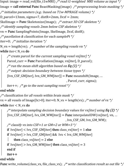
Overview of the proposed algorithm in pseudocode.
EXPERIMENTS
Dataset Description
T1‐weighted MRI data of 15‐healthy individuals (7 males; mean ± SD age = 29 ± 10 years) were acquired on a 3.0 Tesla Siemens Magnetom TimTrio System with a 32 phased‐array receiver head coil using a 3D‐MPRAGE sequence (TR = 2,300 ms; TE = 2.98 ms; TI = 900 ms; flip angle = 9°; matrix size = 256 × 256; FOV = 256 × 256 mm2), resulting in isotropic 1 × 1 × 1 mm3 voxels. None of the subjects had a mass lesion (malformation of cortical development, tumor, or vascular malformation) or a history of traumatic brain injury. The Ethics Committee of the Montreal Neurological Institute and Hospital approved the study, and written informed consent was obtained from all participants.
We also evaluated our method on 1.5 Tesla data of 20‐healthy individuals (8 males; mean ± SD age = 23 ± 4 years) from the Open Access Series of Imaging Studies (OASIS; http://www.oasis-brains.org /). Images were acquired using a 3D‐MPRAGE sequence (TR = 9.7 ms; TE = 4 ms; TI = 20 ms; flip angle = 10°; matrix size = 256 × 256; FOV = 256 × 256 mm2, resulting in 1 × 1 × 1.25 mm3 voxels).
Ground Truth: Reference Segmentation
For the 3.0 Tesla dataset, all 15 subjects had manually labeled whole‐brain GM, WM, and CSF available, drawn by a single rater (JWH). Another rater (SJH) separately labeled a subset of 6 randomly chosen cases, blinded to the labels drawn by JWH. In central and occipital cortices where bright GM intensities are caused by large myelination of deep cortical layers, 3D orthogonal viewing allowed two raters to identify a visible border between GM and WM with a higher gradient than surrounding voxels. As our purpose was cortical tissue classification, we masked out subcortical regions including the basal ganglia, thalamus, and ventricles by the ANIMAL algorithm, a multiresolution nonlinear warping of an atlas that was manually drawn on the MNI‐ICBM 152 template [Collins et al., 1999].
To quantify inter‐rater variability, we calculated the Dice overlap index:
| (3) |
Where M 1 is the segmentation of Rater 1, M 2 the segmentation of Rater 2; M 1 ∩ M2 the voxel‐wise intersection of M 1 and M 2; and v(·) the volume operator. Mean ± SD inter‐rater reliability was 99.1 ± 0.4% for GM and 99.3 ± 0.3% for WM. For the 1.5 Tesla OASIS dataset, only manual labeling of the neocortical GM was available.
Parameter Sensitivity Analysis and Optimization
Parameter optimization was carried out in each dataset (i.e., 3.0 Tesla; 1.5 Tesla) separately. The following parameters were chosen empirically: D parcel as the extent of brain parcels from the sampling point of reference; σ as the mean‐shift kernel bandwidth; R as the distance between sampling points. Classification was evaluated using a threefold cross‐validation. We randomly assigned our subjects to three sets of similar size (n = 5 for 3.0 Tesla; n = 6, 7, and 7 for 1.5 Tesla). A single subsample was selected as test‐set and the two remaining subsamples as training data. We selected those parameters that maximized the overlap between automated and manual segmentations in the training‐set, and computed segmentation accuracy in the test‐set to validate. This process was repeated three times to evaluate across all three subsets.
Performance Comparison with state‐of‐the‐Art Algorithms
We compared our classification against the following approaches: (i) Nonlocal fuzzy C‐means (NLFCM), which generates a cubic volume centered at every voxel inside the brain and assigns tissue memberships to the center voxel by combining clustering with nonlocal smoothing [Caldairou et al., 2011]; (ii) SPM8, based on a Bayesian framework which combines a mixture of Gaussian distribution models and a prior model to constrain spatially varying intensity nonuniformity and shape deformations [Ashburner and Friston, 2005]; and (iii) FSL‐FAST (ver. 4.1), based on a Hidden Markov Random Field Model and the Expectation Maximization algorithm [Zhang et al., 2001].
Default parameters provided in each algorithm did not always result in the most accurate segmentations when using our data. Thus, for fair comparison, optimal parameters were empirically selected using threefold cross‐validation, as in the parameter optimization of our algorithm. As SPM8 and FSL‐FAST incorporate their own intensity inhomogeneity corrections, parameters specific to these processes were also optimized empirically.
Performance Relative to Manual Labeling
Global overlap assessment
To quantify the volume‐wise accuracy of our approach, we computed the Dice overlap between Manual labeling and Automatic labeling, as in Eq. (3). To measure global contour differences between manual and automated labeling, we computed the mean Hausdorff distance, Hm [Chupin et al., 2007; Kim et al., 2012]:
| (4) |
where S M and v M is the surface boundary and its voxels for the manual label, S A and v A the surface boundary and its voxels for the automatic label; d(.,.) is the shortest distance defined by the Euclidean distance. We measured Hm separately for GM/WM and GM/CSF interfaces.
Surface‐based local analysis of contour accuracy
To localize the mis‐segmentation, a surface‐based framework was used to spatially localize contour difference between manual and automated segmentations [Kim et al., 2005; Worsley et al., 2009]. We automatically extracted parametric surface models of the GM–WM interfaces based on the manual labels, and based on the tissue classifications of each automated algorithm [Kim et al., 2005]. To this end, we deformed an ellipsoid triangulated using multiresolution icosahedral sampling [Kim et al., 2005], which allowed a fast fitting while avoiding a possible problem of local minima. The initial surface was sampled with 320 triangles and deformed towards the boundary of a hemispheric WM while maintaining intervertex distance and triangular topology. The surface was up‐sampled at the end of each deformation cycle, up to 81,920 triangles. We did not extract GM–CSF interface as this process required additional morphological operations on top of the given segmentation, likely modifying the actual boundary. Individual surfaces were aligned to a symmetric template [Lyttelton et al., 2007] using a nonlinear surface registration [Robbins et al., 2004]. Note that the realignment did not change the original surface morphology but only relocated vertices on the surface based on the curvature of the cortical surface to provide point‐wise correspondence between automated and manual segmentation. For each classification algorithm, we computed the point‐wise surface‐normal component of the displacement vector between automated and manual labels and performed surface‐based t‐tests on these differences [Worsley et al., 2009]. To improve statistical sensitivity and across‐subject correspondence, data were blurred using a surface‐based diffusion kernel of 10 mm full‐width‐at‐half‐maximum (FWHM). To correct for multiple comparisons, we corrected significances using random field theory, thereby controlling the family‐wise error (FWE) to be below 0.01 [Worsley et al., 1999].
Robustness against intensity nonuniformity
Classification accuracy is often dependent on preprocessing of intensity inhomogeneity correction. A nonoptimized parameter in such correction methods may yield undesirable tissue segmentation. We thus assessed each segmentation algorithm with respect to the wavelength of the estimated nonuniformity fields: a main parameter in the intensity inhomogeneity correction. FSL‐FAST was evaluated by varying the smoothing extent parameter in its own bias‐correction, and SPM8 by varying the bias FWHM parameter. The proposed method and NLFCM were evaluated by varying the smoothing distance parameter of a conventional correction method, N3 algorithm [Sled et al., 1998].
Influence of CSF Skeleton on Segmentation
As our algorithm relies on the CSF skeleton that defines the initial GM/CSF interface, we assessed whether the final segmentation improved GM/CSF interface classification against the initial segmentation by computing their mean Hausdorff distances to manual segmentation.
RESULTS
Parameter Optimization
Optimal performance was achieved with the parameters D = 13 mm, σ = 7, and R = 2 mm (note: we obtained an identical result at R = 1 mm. However, the segmentation was computationally more efficient at 2 mm) in each dataset separately (3.0 Tesla, Dice range across the three different evaluations = 97.5–98.1%; 1.5 Tesla OASIS, 89.2–89.4%; Fig. 2).
Figure 2.
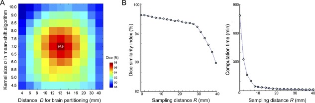
Parameter optimization for the 3.0 Tesla dataset. Classification accuracy was quantified using the Dice index between automated and manual labels. (A) Optimal classification was achieved at a parcel distance of D parcel = 13 mm and a bandwidth kernel size σ = 7 of the mean‐shift clustering. (B) Accuracy was maintained by imposing an intersampling distance pruning of R = 2 mm (left). Accuracy linearly decreased until R = 30 mm, while increasing R exponentially reduced computational complexity (right). [Color figure can be viewed in the online issue, which is available at http://wileyonlinelibrary.com.]
Parameters of all other algorithms were optimized for each dataset separately as explained in the method.
Cross‐Method Comparison
Manual labeling and classification of all evaluated algorithms are shown in Figure 3.
Figure 3.
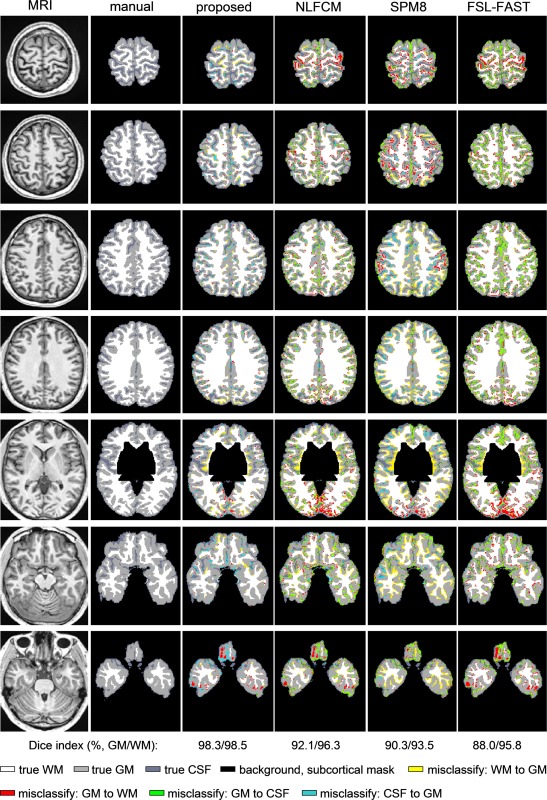
Exemplary tissue classification in an individual brain. Columns display T1‐weighted MRI, manual labels, and automated classification results of the proposed method, NLFCM, SPM8, and FSL‐FAST. [Color figure can be viewed in the online issue, which is available at http://wileyonlinelibrary.com.]
Global assessment
Classification performance is listed in the Table 1. Across the two datasets, our method provided the highest accuracy (3.0 Tesla: t > 11.5, P < 0.001, Bonferroni‐corrected; 1.5 Tesla: t > 10.1, P < 0.001, Bonferroni‐corrected).
Table 1.
Comparison between automated segmentation methods and manual labeling using Dice similarity index (Dice, mean ± SD, in %) and mean Hausdorff distance (Hm, mean ± SD, in mm) for the 3.0 Tesla and 1.5 Tesla datasets
| Proposedskel1 | Proposedskel2 | nonlocal FCM | SPM8 | FSL‐FAST | |
|---|---|---|---|---|---|
| 3 Tesla | |||||
| Dice,GM | 97.9 ± 0.6 | 97.7 ± 0.8 | 91.4 ± 1.0a | 91.1 ± 1.3a | 89.6 ± 1.0a |
| Hm,GM/CSF | 0.21 ± 0.04 | 0.21 ± 0.05 | 0.61 ± 0.13a | 0.43 ± 0.06a | 0.58 ± 0.14a |
| Hm,GM/WM | 0.13 ± 0.02 | 0.13 ± 0.02 | 0.24 ± 0.04a | 0.43 ± 0.05a | 0.27 ± 0.04a |
| 1.5T Tesla | |||||
| Dice,GM | 89.2 ± 0.7 | 89.3 ± 0.6 | 86.7 ± 0.6a | 83.7 ± 1.0a | 81.2 ± 1.7a |
| Hm,GM/CSF | 0.58 ± 0.10 | 0.57 ± 0.09 | 0.59 ± 0.09 | 1.15 ± 0.24a | 1.33 ± 0.28a |
| Hm,GM/WM | 0.32 ± 0.02 | 0.32 ± 0.03 | 0.39 ± 0.02a | 1.10 ± 0.10a | 1.01 ± 0.12a |
Our method's high performance was maintained even with a sparse sampling up to R = 18 mm (Fig. 2; 3.0 Tesla: Dice = 94.1 ± 2.3%; 1.5 Tesla: Dice = 88.3 ± 1.1%). Notably, while sparse sampling decreased computation time from 790 to 9 min for a single scan (Linux workstation, 1 CPU, 2.30 Ghz, 8GB RAM), performance remained superior to the other algorithms, (t < 4.4, P < 0.01 Bonferroni‐corrected).
Our algorithm significantly improved the segmentation accuracy of GM/CSF interface defined by CSF skeletonization (Hm: 0.21 ± 0.04 mm vs. 0.43 ± 0.06 mm, t = 11, P < 0.0001). The choice of CSF skeletonization algorithm did not affect classification performance of our algorithm in the 3T and 1.5T datasets (Table 1; Tohka vs. SPM8, 3T: GM: Dice = 97.9 ± 0.6 vs. 97.7 ± 0.8, Hm, GM/CSF = 0.21 ± 0.04 vs. 0.21 ± 0.05, P > 0.3, FWE; 1.5T OASIS: GM: Dice = 89.2 ± 0.7 vs. 89.3 ± 0.6, Hm, GM/CSF = 0.58 ± 0.10 vs. 0.57 ± 0.09, P > 0.4, FWE). Subsequent evaluations were based on the CSF skeleton based on Tohka's method.
Surface‐based contour accuracy
At the WM–GM interface, all conventional algorithms underestimated central and occipital GM compared to manual labeling (0.7–1.5 mm; Fig. 4). Our algorithm segmented these areas very well (displacement: <0.3 mm) When mis‐segmentation was compared between the proposed algorithm and others, our algorithm indeed showed more significantly superior performance (FWE < 0.001). SPM8 and FSL‐FAST furthermore showed lower accuracy in anterior temporal and frontal regions (FWE < 0.01).
Figure 4.
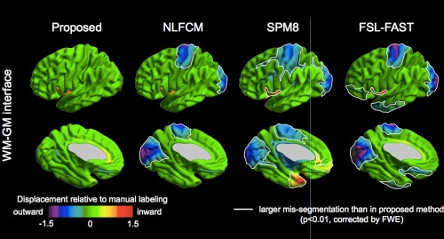
Contour analysis. Surface maps show mean displacement of automated algorithms compared to manual segmentation (in mm). Significantly larger displacements (i.e., increased segmentation errors) of NLFCM, SPM8, and FSL‐FAST compared to the proposed algorithm, corrected for multiple comparisons using random field theory for nonisotropic images at FWE < 0.01, are highlighted by white borders. [Color figure can be viewed in the online issue, which is available at http://wileyonlinelibrary.com.]
Robustness against intensity‐inhomogeneity
Performance of the proposed method and NLFCM was independent from the bandwidth parameter of nonuniformity correction (i.e., N3) (r < 0.12, t < 1.3, P > 0.1, uncorrected; Fig. 5). Conversely, classification accuracy of SPM8 and FSL‐FAST decreased with larger wavelength of their own correction methods (r > 0.5, t > 3.4, P < 0.005, Bonferroni‐correction).
Figure 5.
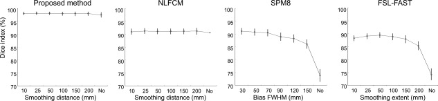
Impact of intensity inhomogeneity correction parameters on automated classification. Each algorithm was tested at various smoothing distance parameters, or without correction. For SPM8 and FSL‐FAST, we used their integrated correction routine; our method and NLFCM were tested using the N3 algorithm [Sled et al., 1998]. While global methods (i.e., SPM8, FSL‐FAST) showed reduced performance when no bias correction was chosen, local classification algorithms (i.e., the proposed method and NLFCM) maintained high accuracy irrespective of the correction parameters.
DISCUSSION
MRI intensities within a given tissue type are subject to considerable nonuniformity across the brain, challenging the mapping from intensity values to classes. One source of inhomogeneity relates to poor radio frequency coil uniformity and gradient‐driven eddy currents. While several preprocessing strategies have been developed to reduce such intensity bias [Ashburner and Friston, 2005; Sled et al., 1998], correction parameters and their efficacy may vary across datasets and magnetic field strengths [Boyes et al., 2008]. Aside from MRI‐related artifacts, neuroimaging investigations on normal brain anatomy have shown substantial signal variations in T1 or T1‐weighted images that are of biological origin, with a darker appearance of association cortices relative to bright‐appearing primary sensory and motor cortices [Dinse et al., 2013; Fischl et al., 2004; Salat et al., 2009; Steen et al., 2000]. In the light of early neuroanatomical work on cortical myeoloarchitecture [Flechsig, 1920; Vogt, 1910], and correlative studies, it has become increasingly evident that T1 and T1‐weighted signal strongly relates to cortical myelin content, which has been shown to vary substantially across cortical regions [Bock et al., 2013; Eickhoff et al., 2005; Geyer et al., 2011; Glasser and Van Essen, 2011].
In this work, we present a novel tissue classification algorithm that created anatomically constrained local parcels from the brain, instead of operating over the entire image. The success of local tissue classification is highly related to the size and shape of the formed parcels. On the one hand, parcels should be sufficiently large to sample adequate amount of tissue, yet small enough to avoid intensity bias effects. Moreover, consistency across neighboring parcels needs to be guaranteed. Previous techniques based on use of cubic parcels used voxel‐wise local Gaussian mixtures [Grabowski et al., 2000; Joshi et al., 1999] or an interpolation of partially overlapping models [Grabowski et al., 2000]. More recent approaches have combined Gaussian mixtures and cooperative local Markov random fields [Richard et al., 2007; Scherrer et al., 2009] to ensure smooth transitions; others have used combinations of multicontext FCM with information fusion [Zhu and Jiang, 2003], or local FCM models with nonlocal means [Caldairou et al., 2011]. The latter approach, NLFCM [Caldairou et al., 2011], is forced to use wide cubes to obtain a reasonable balance of tissue classes, which in turn increases sensitivity to intensity inhomogeneity. In our evaluation, while NLFCM reduced segmentation errors in central and occipital regions compared to SPM and FSL‐FAST, it could not completely eliminate them. On the other hand, the proposed algorithm incorporates sulco‐gyral information through a preliminary CSF skeleton, which allowed the generation of small parcels adhering to cortical topology, while ensuring balanced tissue proportions; notably, the skeleton initialized the placement of the sample points; it was not used for final tissue classification. Since parcels have a small number of voxels, we opted for the nonparametric mean‐shift clustering to obtain modes of the parcel‐wise intensity distributions. This robust method allows not only finding local modes but also local thresholds between two tissue classes. In our approach, consistency across neighboring parcels was obtained by interpolating these thresholds across all brain voxels to provide the final segmentation.
Using comprehensive evaluations against a validated manually labeled dataset (i.e., 20 cases scanned at 3.0 Tesla), we showed excellent overall accuracy to segment GM, WM, and CSF surrounding the cortical ribbon, irrespective of the correction of intensity inhomogeneity. Noteworthy, compared to two widely used algorithms in which tissue classes are estimated from global intensity histograms across the entire volume (i.e., SPM8 and FSL‐FAST), our algorithm showed increased accuracy. Further confidence in the generalizability of our approach derives from its highest performance in an independent 1.5T dataset among the tested algorithms. Surface‐based contour analysis between gold standard and automatic segmentations across thousands of cortical points localized regions of improved performance primarily at the GM/WM boundary of central and occipital cortices, even after conservative correction for multiple comparisons. These findings confirm our hypothesis that local classification accounts for a more flexible differentiation between highly myelinated GM and its underlying WM.
Biomarkers of structural brain integrity have been increasingly applied to develop novel diagnostic, monitoring, and treatment strategies in various neurological conditions. The excellent performance of the proposed anatomy‐driven local classification method advocates for its use in the study of the healthy and diseased brain.
Our segmentation was optimized to segment GM/WM near the cortex. Decision boundaries were regionally determined at every sample points extracted along the neocortex including the insula and the mesial temporal lobe. These values were then interpolated to all other brain regions including the brainstem, deep GM structures and midsagittal WM. Accordingly their decision boundary values were determined by the interpolation of neocortical samples. We found that non‐neocortical segmentation was quite similar to that determined by the global classification. A further study that expands our sampling scheme to these structures may improve their segmentation.
The parameters in the proposed tissue classification were optimized empirically on each 1.5T and 3T dataset separately. As a result, parameters could have been different between the two datasets. However, the parameters resulting in the best performance for both datasets were identical. Even though the two datasets were scanned in different field strength, a same imaging sequence (i.e., 3D‐MPRAGE) and a same preprocessing that corrected for intensity inhomogeneity, and performed registration and resampling were applied to the both datasets. This may explain that the imaging sequence and image preprocessing would be more important factors to determine the classification parameters than the MRI field strength. The field strength is yet associated with the classification performance as the accuracy was higher in the 3T dataset than the 1.5T dataset. It is noted that some parameters (D CSF, 3 mm dilation to include CSF voxels in parcels) should be carefully chosen based on the cortical thickness or the sample balance between tissue types. Also, D parcel related to the size of the used parcels should be chosen as small as to prevent from inclusion of tissues from multiple cortices.
REFERENCES
- Ashburner J, Friston KJ (2005): Unified segmentation. Neuroimage 26:839–851. [DOI] [PubMed] [Google Scholar]
- Bernhardt BC, Bernasconi N, Concha L, Bernasconi A (2010): Cortical thickness analysis in temporal lobe epilepsy: Reproducibility and relation to outcome. Neurology 74:1776–1784. [DOI] [PubMed] [Google Scholar]
- Bock NA, Hashim E, Janik R, Konyer NB, Weiss M, Stanisz GJ, Turner R, Geyer S (2013): Optimizing T(1)‐weighted imaging of cortical myelin content at 3.0T. Neuroimage 65:1–12. [DOI] [PubMed] [Google Scholar]
- Boyes RG, Gunter JL, Frost C, Janke AL, Yeatman T, Hill DLG, Bernstein MA, Thompson PM, Weiner MW, Schuff N, Alexander GE, Killiany RJ, DeCarli C, Jack CR, Fox NC (2008): Intensity non‐uniformity correction using N3 on 3‐T scanners with multichannel phased array coils. Neuroimage 39:1752–1762. [DOI] [PMC free article] [PubMed] [Google Scholar]
- Caldairou B, Passat N, Habas PA, Studholme C, Rousseau F (2011): A non‐local fuzzy segmentation method: Application to brain MRI. Pattern Recognit 44:1916–1927. [Google Scholar]
- Chupin M, Mukuna‐Bantumbakulu AR, Hasboun D, Bardinet E, Baillet S, Kinkingnehun S, Lemieux L, Dubois B, Garnero L (2007): Anatomically constrained region deformation for the automated segmentation of the hippocampus and the amygdala: Method and validation on controls and patients with Alzheimer's disease. Neuroimage 34:996–1019. [DOI] [PubMed] [Google Scholar]
- Collins DL, Zijdenbos AP, Baare WFC, Evans AC (1999): ANIMAL+INSECT: Improved cortical structure segmentation In: Kuba A, editor. Image Processing in Medical Imaging. Springer Verlag, Heidelberg, Cambridge, UK: pp 210–223. [Google Scholar]
- Colliot O, Bernasconi N, Khalili N, Antel SB, Naessens V, Bernasconi A (2006): Individual voxel‐based analysis of gray matter in focal cortical dysplasia. Neuroimage 29:162–171. [DOI] [PubMed] [Google Scholar]
- Comaniciu D, Meer P (2002): Mean shift: A robust approach toward feature space analysis. IEEE Trans Pattern Anal Mach Intell 24:603–619. [Google Scholar]
- Dinse J, Waehnert M, Tardif CL, Schafer A, Geyer S, Turner R, Bazin PL (2013): A histology‐based model of quantitative T1 contrast for in‐vivo cortical parcellation of high‐resolution 7 Tesla brain MR images. Med Image Comput Comput Assist Interv 16:51–58. [DOI] [PubMed] [Google Scholar]
- Eickhoff S, Walters NB, Schleicher A, Kril J, Egan GF, Zilles K, Watson JD, Amunts K (2005): High‐resolution MRI reflects myeloarchitecture and cytoarchitecture of human cerebral cortex. Hum Brain Mapp 24:206–215. [DOI] [PMC free article] [PubMed] [Google Scholar]
- Eskildsen SF, Coupe P, Fonov V, Manjon JV, Leung KK, Guizard N, Wassef SN, Ostergaard LR, Collins DL (2012): BEaST: Brain extraction based on nonlocal segmentation technique. Neuroimage 59:2362–2373. [DOI] [PubMed] [Google Scholar]
- Fischl B, Salat DH, van der Kouwe AJ, Makris N, Segonne F, Quinn BT, Dale AM (2004): Sequence‐independent segmentation of magnetic resonance images. Neuroimage 23(Suppl. 1):S69–S84. [DOI] [PubMed] [Google Scholar]
- Flechsig P (1920): Anatomie des menschlichen Gehirns und Rueckenmarks auf myelogenetischer Grundlage. Leipzig: George Thieme.
- Geyer S, Weiss M, Reimann K, Lohmann G, Turner R (2011): Microstructural Parcellation of the human cerebral cortex ‐ from Brodmann's post‐mortem map to in vivo mapping with high‐field magnetic resonance imaging. Front Hum Neurosci 5:19 [DOI] [PMC free article] [PubMed] [Google Scholar]
- Glasser MF, Van Essen DC (2011): Mapping human cortical areas in vivo based on myelin content as revealed by T1‐ and T2‐weighted MRI. J Neurosci 31:11597–11616. [DOI] [PMC free article] [PubMed] [Google Scholar]
- Grabowski TJ, Frank RJ, Szumski NR, Brown CK, Damasio H (2000): Validation of partial tissue segmentation of single‐channel magnetic resonance images of the brain. NeuroImage 12:640–656. [DOI] [PubMed] [Google Scholar]
- Hong SJ, Kim H, Schrader D, Bernasconi N, Bernhardt BC, Bernasconi A (2014): Automated detection of cortical dysplasia type II in MRI‐negative epilepsy. Neurology 83:48–55. [DOI] [PMC free article] [PubMed] [Google Scholar]
- Jenkinson M, Beckmann CF, Behrens TE, Woolrich MW, Smith SM (2012): Fsl. Neuroimage 62:782–790. [DOI] [PubMed] [Google Scholar]
- Joshi M, Cui J, Doolittle K, Joshi S, Van Essen D, Wang L, Miller MI (1999): Brain segmentation and the generation of cortical surfaces. NeuroImage 9:461–476. [DOI] [PubMed] [Google Scholar]
- Kim H, Chupin M, Colliot O, Bernhardt BC, Bernasconi N, Bernasconi A (2012): Automatic hippocampal segmentation in temporal lobe epilepsy: Impact of developmental abnormalities. Neuroimage 59:3178–3186. [DOI] [PubMed] [Google Scholar]
- Kim JS, Singh V, Lee JK, Lerch J, Ad‐Dab'bagh Y, MacDonald D, Lee JM, Kim SI, Evans AC (2005): Automated 3‐D extraction and evaluation of the inner and outer cortical surfaces using a Laplacian map and partial volume effect classification. Neuroimage 27:210–221. [DOI] [PubMed] [Google Scholar]
- Lerch JP, Pruessner JC, Zijdenbos A, Hampel H, Teipel SJ, Evans AC (2005): Focal decline of cortical thickness in Alzheimer's disease identified by computational neuroanatomy. Cereb Cortex 15:995–1001. [DOI] [PubMed] [Google Scholar]
- Lu GY, Wong DW (2008): An adaptive inverse‐distance weighting spatial interpolation technique. Comput Geosci 34:1044–1055. [Google Scholar]
- Lyttelton O, Boucher M, Robbins S, Evans A (2007): An unbiased iterative group registration template for cortical surface analysis. Neuroimage 34:1535–1544. [DOI] [PubMed] [Google Scholar]
- Ma C‐M, Wan S‐Y, Lee J‐D (2002): Three‐dimensional topology preserving reduction on the 4‐subfields. IEEE Trans. Pattern Anal Mach Intell 24:1594–1605. [Google Scholar]
- Richard N, Dojat M, Garbay C (2007): Distributed Markovian segmentation: Application to MR brain scans. Pattern Recognit 40:3467–3480. [Google Scholar]
- Robbins S, Evans AC, Collins DL, Whitesides S (2004): Tuning and comparing spatial normalization methods. Med Image Anal 8:311–323. [DOI] [PubMed] [Google Scholar]
- Salat DH, Lee SY, van der Kouwe AJ, Greve DN, Fischl B, Rosas HD (2009): Age‐associated alterations in cortical gray and white matter signal intensity and gray to white matter contrast. Neuroimage 48:21–28. [DOI] [PMC free article] [PubMed] [Google Scholar]
- Sanchez‐Panchuelo, R.M , Besle, J , Mougin, O , Gowland, P , Bowtell, R , Schluppeck, D , Francis, S (2014): Regional structural differences across functionally parcellated Brodmann areas of human primary somatosensory cortex. Neuroimage 93(Pt 2):221–230. [DOI] [PubMed] [Google Scholar]
- Scherrer B, Forbes F, Garbay C, Dojat M (2009): Distributed Local MRF Models for Tissue and Structure Brain Segmentation. IEEE Trans Med Imaging 28:1278–1295. [DOI] [PubMed] [Google Scholar]
- Sereno MI, Lutti A, Weiskopf N, Dick F (2013): Mapping the human cortical surface by combining quantitative T(1) with retinotopy. Cereb Cortex 23:2261–2268. [DOI] [PMC free article] [PubMed] [Google Scholar]
- Sled JG, Zijdenbos AP, Evans AC (1998): A nonparametric method for automatic correction of intensity nonuniformity in MRI data. IEEE Trans Med Imaging 17:87–97. [DOI] [PubMed] [Google Scholar]
- Steen RG, Reddick WE, Ogg RJ (2000): More than meets the eye: Significant regional heterogeneity in human cortical T1. Magn Reson Imaging 18:361–368. [DOI] [PubMed] [Google Scholar]
- Tam RC, Traboulsee A, Riddehough A, Sheikhzadeh F, Li DK (2011): The impact of intensity variations in T1‐hypointense lesions on clinical correlations in multiple sclerosis. Mult Scler 17:949–957. [DOI] [PubMed] [Google Scholar]
- Tohka J, Zijdenbos A, Evans A (2004): Fast and robust parameter estimation for statistical partial volume models in brain MRI. Neuroimage 23:84–97. [DOI] [PubMed] [Google Scholar]
- Tustison NJ, Avants BB, Cook PA, Zheng Y, Egan A, Yushkevich PA, Gee JC (2010): N4ITK: Improved N3 bias correction. IEEE Trans Med Imaging 29:1310–1320. [DOI] [PMC free article] [PubMed] [Google Scholar]
- Vogt BA (1910): Die Myeloarchitektonische Felderung Des Menschlichen Stirnhirns. Psychologie Und Neurologie 15:221–232. [Google Scholar]
- Worsley KJ, Andermann M, Koulis T, MacDonald D, Evans AC (1999): Detecting changes in nonisotropic images. Hum Brain Mapp 8:98–101. [DOI] [PMC free article] [PubMed] [Google Scholar]
- Worsley KJ, Taylor JE, Carbonell F, Chung MK, Duerden E, Bernhardt B, Lyttelton O, Boucher M, Evans A.C (2009): SurfStat: A Matlab toolbox for the statistical analysis of univariate and multivariate surface and volumetric data using linear mixed effects models and random field theory. NeuroImage 47(Suppl. 1):S102. [Google Scholar]
- Zhang Y, Brady M, Smith S (2001): Segmentation of brain MR images through a hidden Markov random field model and the expectation‐maximization algorithm. IEEE Trans Med Imaging 20:45–57. [DOI] [PubMed] [Google Scholar]
- Zheng W, Chee MW, Zagorodnov V (2009): Improvement of brain segmentation accuracy by optimizing non‐uniformity correction using N3. Neuroimage 48:73–83. [DOI] [PubMed] [Google Scholar]
- Zhu C, Jiang T (2003): Multicontext fuzzy clustering for separation of brain tissues in magnetic resonance images. NeuroImage 18:685–696. [DOI] [PubMed] [Google Scholar]