

Abstract
Multi‐atlas based methods have been recently used for classification of Alzheimer's disease (AD) and its prodromal stage, that is, mild cognitive impairment (MCI). Compared with traditional single‐atlas based methods, multiatlas based methods adopt multiple predefined atlases and thus are less biased by a certain atlas. However, most existing multiatlas based methods simply average or concatenate the features from multiple atlases, which may ignore the potentially important diagnosis information related to the anatomical differences among different atlases. In this paper, we propose a novel view (i.e., atlas) centralized multi‐atlas classification method, which can better exploit useful information in multiple feature representations from different atlases. Specifically, all brain images are registered onto multiple atlases individually, to extract feature representations in each atlas space. Then, the proposed view‐centralized multi‐atlas feature selection method is used to select the most discriminative features from each atlas with extra guidance from other atlases. Next, we design a support vector machine (SVM) classifier using the selected features in each atlas space. Finally, we combine multiple SVM classifiers for multiple atlases through a classifier ensemble strategy for making a final decision. We have evaluated our method on 459 subjects [including 97 AD, 117 progressive MCI (p‐MCI), 117 stable MCI (s‐MCI), and 128 normal controls (NC)] from the Alzheimer's Disease Neuroimaging Initiative database, and achieved an accuracy of 92.51% for AD versus NC classification and an accuracy of 78.88% for p‐MCI versus s‐MCI classification. These results demonstrate that the proposed method can significantly outperform the previous multi‐atlas based classification methods. Hum Brain Mapp 36:1847–1865, 2015. © 2015 Wiley Periodicals, Inc.
Keywords: multiatlas classification, feature selection, Alzheimer's disease, ensemble learning, multiview learning
INTRODUCTION
As the most common form of dementia diagnosed in people over 65 years of age, Alzheimer's disease (AD) is an irreversible, neurodegenerative disorder that leads to progressive loss of memory and cognitive function. It is reported that, 1 in 85 people will be affected by AD by 2050 [Brookmeyer et al., 2007]. Thus, it is critical for early and accurate diagnosis of AD, especially in its early stage [i.e., mild cognitive impairment (MCI)], for timely therapy and possible delay of the progression [Li et al., 2012; Wee et al., 2012; Wee et al., 2014; Zhang et al., 2012].
Over the past decade, advances in magnetic resonance imaging (MRI) have enabled significant progress in understanding neural changes that are related to AD and other diseases [Chan et al., 2003; Chen et al., 2009b; Davatzikos et al., 2008; Fan et al., 2008; Fox et al., 1996; Hinrichs et al., 2009; Magnin et al., 2009; Mueller et al., 2005; Shi et al., 2012]. By directly accessing the structures provided by MRI, brain morphometry can identify the anatomical differences between populations of AD patients and normal controls (NC) for assisting diagnosis and also evaluating the progression of MCI [Dickerson et al., 2001; Fox et al., 1996; Jack et al., 2008; Wang et al., 2014]. In general, MRI‐based classification methods can be roughly divided into two categories, that is, (1) methods using single‐atlas based morphometric representations of brain structures [Cuingnet et al., 2011; Liu et al., 2014; Zhang et al., 2011] and (2) methods using multi‐atlas based representations of brain structures [Koikkalainen et al., 2011; Leporé et al., 2008; Min et al., 2014a, 2014b].
In the first category of methods, researchers mainly utilize a single atlas as a benchmark space to provide a representative basis for comparing the common anatomical structures of different brain images. More specifically, they first obtain a morphometric representation of each brain image by spatially normalizing it onto a common space (i.e., a predefined atlas) via nonlinear registration, and thus, the corresponding regions in different brain images can be compared [Sotiras et al., 2013; Tang et al., 2009; Yap et al., 2009]. Usually, such a predefined atlas is an image of a single subject, a general average atlas, or a specific atlas generated from a particular data under study [Chung et al., 2001; Leporé et al., 2008; Teipel et al., 2007]. In the literature, many single‐atlas based morphometry pattern analysis methods, such as voxel‐based morphometry (VBM) [Ashburner and Friston, 2000; Davatzikos et al., 2001, 2008; Thompson et al., 2001], deformation‐based morphometry (DBM) [Ashburner et al., 1998; Chung et al., 2001; Gaser et al., 2001; Joseph et al., 2014], and tensor‐based morphometry (TBM) [Kipps et al., 2005; Leow et al., 2006; Whitford et al., 2006], have been proposed and demonstrated promising results in AD diagnosis with different classification techniques [Bozzali et al., 2006; Fan et al., 2008; Frisoni et al., 2002; Hua et al., 2013]. Specifically, in these methods, after nonrigidly transforming each individual brain image onto a common atlas space, VBM measures the local tissue density of the original brain image directly, while DBM and TBM measure the local deformation and the Jacobian of local deformation, respectively. For example, researchers in [Fan et al., 2007] proposed a Classification Of Morphological Patterns using Adaptive Regional Elements (COMPARE) algorithm to extract volumetric features from self‐organized and spatially adaptive local regions based on a single atlas. COMPARE helps overcome the limitation of traditional voxel‐wise analysis methods that often have very high feature dimensionality, and can also enhance the discriminative power of the feature representation. However, due to the potential bias associated with the use of a particular atlas, the feature representation extracted from a single (particular) atlas may not be sufficient to reveal the underlying complicated differences between populations of disease‐affected patients and NCs.
In the second category of methods, researchers attempt to use multiple atlases to minimize the bias associated with the use of a single atlas. Although requiring higher computational cost, this kind of method is important for helping reduce the negative impact of image registration errors in morphometric analysis of brain images. Recently, several studies [Koikkalainen et al., 2011; Leporé et al., 2008; Min et al., 2014a, 2014b] have shown that the multiatlas based methods can often offer more accurate diagnosis results than the single‐atlas based methods. For example, researchers in [Leporé et al., 2008] registered each brain image onto multiple atlases (which have already been nonlinearly aligned to a new common atlas), and then averaged their respective Jacobian maps of the estimated deformation fields to improve the TBM‐based monozygotic/dizygotic twin classification. To reduce errors caused by registration in the TBM‐based classification, researchers in [Koikkalainen et al., 2011] investigated the effects of utilizing mean deformation fields, mean volumetric features, and mean predicted responses of regression‐based classifiers from multiple atlases, and obtained the improved results for AD analysis. However, one main disadvantage of the aforementioned methods is that, after averaging the features from multiple atlases, morphometric representations for a subject (although generated from different atlases) could become less powerful in revealing the underlying complicated differences between AD patients and NCs, because they ignore the characteristics of each atlas.
It is worth noting that, because the anatomical structures of different atlases could be very different from each other, a subject's corresponding representations generated from different atlases (also called views later) will also be different, as illustrated in Figure 1. From Figure 1, we can observe that the gray matter (GM) tissue density maps represented in the spaces of two atlases (i.e., Ti and Tj) are very different. Therefore, the representations generated from these different atlases [Min et al., 2014b] would convey different information to help reveal the underlying complicated differences between populations of disease‐affected patients and NCs. To this end, researchers in [Min et al., 2014a, 2014b] proposed to nonlinearly register each brain image onto multiple atlases separately for obtaining multiple representations. However, in [Min et al., 2014a, 2014b], when considered for AD classification, the features generated from different atlases are simply concatenated, which could include redundant information from similar atlases and also lead to high dimensional feature representations. Therefore, deciding how to better use those feature representations from multiple atlases is a challenging problem.
Figure 1.
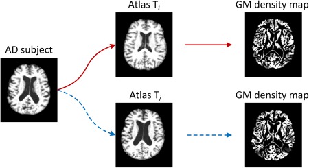
Illustration of different morphometric patterns generated from different atlases. Here, an AD subject image is registered to two different atlases (i.e., Ti and Tj), through which two different representations (i.e., density maps for GM) are generated as features for the AD subject. [Color figure can be viewed in the online issue, which is available at http://wileyonlinelibrary.com.]
Conversely, in machine learning and pattern recognition domains, multiview based learning methods have been well studied to make full use of features from multiple views to represent an object [Li et al., 2002; Thomas et al., 2006]. For example, in the multiview face recognition, a person can be represented by both front‐view and side‐view images. Because these images provide different information for the same person, the use of multiple sets of features from different views can largely enrich the representation for the person and bring better learning performance than methods with only single‐view features, as demonstrated in various studies [Basha et al., 2013; Gong et al., 2014; Li et al., 2002; Thomas et al., 2006; Xu et al., 2014]. Similarly, in brain morphometry, multiple atlases can also be regarded as multiple views for representing the same brain. Thus, a representation generated from a specific atlas can be regarded as a profile for the brain, and can be used to provide supplementary or side information for other representations generated from the other atlases (i.e., views). Intuitively, focusing on the representation from one atlas with also extra guidance from other atlases could lead to a richer representation for the brain, and thus improve the disease diagnosis performance. However, to our knowledge, few of the existing multiatlas based classification methods have explored the representation of each atlas with extra guidance from other atlases to aid more accurate classification of AD or related brain disease(s).
In this article, we propose a view‐centralized multi‐atlas (VCMA) classification method to identify (1) AD patients from NCs and (2) progressive MCI patients from stable MCI patients, using a collection of representations derived from multiple atlases. Unlike previous multiatlas based works in [Koikkalainen et al., 2011; Leporé et al., 2008] that often averaged the representations from multiple atlases, or works in [Min et al., 2014a, 2014b] that simply concatenated features from different atlases, we retain each atlas in its original (linearly aligned) space and then focus on the feature representation from each atlas with extra guidance provided by other atlases. The key of our proposed method involves a VCMA feature selection algorithm and also a classifier ensemble strategy. Specifically, we first spatially normalize each brain image onto multiple atlases via nonlinear registration for obtaining the respective regional features in multiple atlases. Then, we propose a VCMA feature selection method by concentrating on the feature representation of each atlas with extra guidance from other atlases. Here, for a certain atlas, we treat it as the main‐view information source, and regard other atlases as the side‐view information sources for providing extra side information for the main‐view. As each of the K atlases will be treated as the main‐view (with other K−1 atlases as side views), in turn, our proposed VCMA feature selection method will be performed for K times to get K sets of selected features. Finally, based on these K sets of selected features, support vector machine (SVM) classifiers [Jie et al., 2014; Klöppel et al., 2008; Magnin et al., 2009; Zhang et al., 2011] are learned to construct multiple (i.e., K) base classifiers, and then these K base classifiers are combined through a classifier ensemble strategy for making a final decision. To evaluate the efficacy of our proposed method, we perform two sets of experiments: (1) AD versus NC classification and (2) progressive MCI (p‐MCI) versus stable MCI (s‐MCI) classification. Using a 10‐fold cross‐validation strategy on the Alzheimer's Disease Neuroimaging Initiative (ADNI) database [Jack et al., 2008], we achieve a significant performance improvement for both AD versus NC classification and p‐MCI versus s‐MCI classification, compared with the state‐of‐the‐art methods for AD/MCI diagnosis.
The rest of this article is organized as follows. The proposed VCMA classification method is presented in the Method section. Then, in the Results section, we perform extensive experiments by comparing our method with several state‐of‐the‐art methods using the ADNI database. Finally, in the Conclusion section, we conclude this paper and discuss some possible future directions.
METHOD
Figure 2 shows the flowchart of our proposed view‐centralied multi‐atlas (VCMA) classification framework. As can be seen from Figure 2, brain images are first nonlinearly registered onto multiple atlases individually, and then, their volumetric features are extracted within each atlas space. In this way, multiple feature representations can be generated from different atlases for each specific subject. Based on such representations, we then apply our proposed VCMA feature selection algorithm to select the most discriminative features, by focusing on the main‐view atlas along with the extra guidance from side‐view atlases. Finally, multiple SVM classifiers are constructed based on multiple sets of selected features, followed by a classifier ensemble strategy to combine the outputs of multiple SVM classifiers for making a final decision. In what follows, we will introduce each step in detail.
Figure 2.
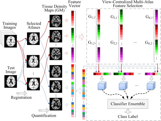
The framework of our proposed view‐centralized multi‐atlas classification method, which includes four main steps: (1) preprocessing and atlas selection, (2) feature extraction, (3) feature selection, and (4) ensemble classification. [Color figure can be viewed in the online issue, which is available at http://wileyonlinelibrary.com.]
Preprocessing and Atlas Selection
For all studied subjects, we first apply a standard preprocessing procedure to the T1‐weighted MR brain images. More specifically, nonparametric nonuniform bias correction (N3) [Sled et al., 1998] is used to correct intensity in homogeneity. Then, we perform skull stripping [Wang et al., 2014], and also perform manual review (or correction) to ensure the clean removal of skull and dura. Afterward, we remove the cerebellum by warping a labeled atlas to each skull‐stripping image. Next, we apply the FAST method [Zhang et al., 2001] to segment each brain image into three tissues, that is, GM, white matter (WM) and cerebrospinal fluid (CSF). Finally, all brain images are affine‐aligned by FLIRT [Jenkinson et al., 2002; Jenkinson and Smith, 2001].
One challenging problem in multiatlas based methods is deciding how to select appropriate atlases, which should not only be representative enough to cover the entire population, to reduce the overall registration errors, but also capture the discriminative information of brain changes related to AD. For that purpose, we first perform a clustering algorithm, called affinity propagation [Frey and Dueck, 2007], to partition the whole population of AD and NC images into K (e.g., K = 10 in this study) nonoverlapping clusters, through which an exemplar image can be automatically selected for each cluster. Then, these exemplar images can be used as representative images or atlases for different clusters. Accordingly, we can construct an atlas pool by combining these exemplar images from different clusters. During the clustering process, the normalized mutual information [Pluim et al., 2003] is used as similarity measure and a bisection method [Frey and Dueck, 2007] is adopted to find the appropriate preference value for the affinity propagation clustering algorithm. In this study, there are a total of 10 atlases in our atlas pool. Although it is possible to add more atlases to the atlas pool, those additional atlases could introduce redundant information, as well as higher computational cost, especially in the image registration stage. It is worth noting that multiple atlases used in this study are only selected from both AD and NC subjects rather than MCI subjects, because MCI can be regarded as an intermediate stage between AD and NC and, thus, owns the characteristics of both AD and NC.
Feature Extraction
To obtain feature representations for each subject based on multiple atlases, we perform the following two procedures: (1) a registration step for spatial normalization of different brain images onto multiple atlas spaces and (2) a quantification step for morphometric measurement. Specifically, for a given subject with three segmented tissues (i.e., GM, WM, and CSF), its brain image is first nonlinearly registered onto K atlases using a high‐dimensional elastic warping tool, that is, HAMMER [Shen and Davatzikos, 2002]. Then, based on these K estimated deformation fields, for each tissue we quantify its voxel‐wise tissue density map [Davatzikos et al., 2001; Goldszal et al., 1998] in each of the K atlas spaces, to reflect the unique deformation behaviors of a given subject with respect to each specific atlas. In this study, we extract a GM density map as the feature representation for a brain image, as GM is the most affected by AD and widely used in the literature [Liu et al., 2014; Min et al., 2014a; Zhang and Shen, 2012].
After registration and quantification in each atlas space, we first determine a set of region of interest (ROI) by performing watershed segmentation [Grau et al., 2004; Vincent and Soille, 1991] on the correlation map between voxel‐wise tissue density values and class labels of all training subjects. It is worth noting that each atlas will yield its unique ROI partition, as different tissue density maps of the same subject are often generated from different atlas spaces. Then, to improve the discriminative power, as well as the robustness of the volumetric features computed from each ROI, we further refine ROI by choosing the voxels with reasonable representation power. To be specific, we first select the most relevant voxel according to the Pearson correlation (PC) between this voxel's tissue density values and class labels among all training subjects. Then, we iteratively include the neighboring voxels until no increase in PC when adding new voxels. Note that such voxel selection process will lead to a voxel set for a specific region, through which the mean of tissue density values of those selected voxels can be computed as the feature for this region. It is worth noting that such voxel selection process is important in eliminating irrelevant and noisy features, which has been confirmed by several previous studies [Liu et al., 2013; Min et al., 2014a, 2014b]. Finally, in each atlas space, the top 1,500 most discriminative ROI features are selected as the representation for a subject. Given K atlases, the feature representation for each subject is of 1,500 dimensionality.
Feature Selection
Although we extract the most representative regional features in each atlas space, many regional features could still be redundant or too noisy for the subsequent classification task. Therefore, feature selection plays an important role in selecting a robust feature subset, as well as to remove those noisy features to achieve good classification results.
In this subsection, we propose a VCMA feature selection method to select features from each atlas with extra guidance from other atlases. Specifically, given N training images that have been registered to K atlases, we denote (D = 1,500 in this study) as the training data, where is the feature representation generated from K atlases for the ith training image. Let be the class labels of N training data, and be the weight vector for the feature selection task. For clarity, we divide the feature representations from multiple atlases into a main‐view group and a side‐view group, as illustrated in Figure 3. As can be seen from Figure 3, the main‐view group (corresponding to the main atlas) contains features from a certain atlas, while the side‐view group (corresponding to other supplementary atlases) contains features form all other (supplementary) atlases.
Figure 3.
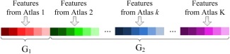
Illustration of group information for feature representations generated from multiple atlases. The first group G1 (i.e., the main‐view group) consists of features from a certain atlas, while the second group G2 (i.e., the side‐view group) contains features from all other (supplementary) atlases. [Color figure can be viewed in the online issue, which is available at http://wileyonlinelibrary.com.]
Denote as the weighting parameters for two different groups, where represents the weighting value for the main‐view (i.e., main atlas) group and denotes the weighting value for the side‐view (i.e., supplementary atlases) group. By setting different weighting values for features from the main view and the side views, we can incorporate our prior information into the following learning model:
| (1) |
where represents the weight vector for the th group. The first term in Eq. (1) is the empirical loss on the training data, and the second one is the L1‐norm regularization term that enforces some elements of to be zero. It is worth noting that the last term in Eq. (1) is a view‐centralized regularization term, which treats features in the main‐view group and the side‐view group differently using different weighting values (i.e., and ). For example, a small (as well as a large ) implies that the coefficients for features in the main‐view group will be penalized lightly, while features in the side‐view group will be penalized severely, because the goal of the model defined in Eq. (1) is to minimize the objective function. Accordingly, most elements in the weight vector corresponding to the side‐view group will be zero, while those corresponding to the main‐view group will not. In this way, the prior knowledge that we focus on the representation from the main atlas (i.e., main view) with extra guidance from other atlases can be incorporated into the learning model naturally. In addition, two constraints in Eq. (1) are used to ensure that the weighting values for different groups are greater than 0 and not greater than 1. By introducing such constraints, we can efficiently reduce the freedom degree of the proposed model, and avoid over‐fitting with limited training samples.
Based on the feature selection model defined in Eq. (1), we can obtain a feature subset by selecting features with non‐zero coefficients in . Each time, we perform the aforementioned feature selection procedure by focusing on one of multiple atlases, with other atlases used as extra guidance. Accordingly, given K atlases, we get K selected feature subsets, with each of them reflecting the information learned from a certain main atlas and corresponding supplementary atlases.
It is straightforward to verify that the objective function in Eq. (1) is convex but nonsmooth because of the nonsmooth L1‐norm regularization term. The basic idea to solve this problem is to use a smooth function to approximate the original nonsmooth objective function and then solve the former by utilizing some off‐the‐shelf fast algorithms. In this study, we resort to the widely used Accelerated Proximal Gradient (APG) method [Beck and Teboulle, 2009; Chen et al., 2009b] to solve the problem defined in Eq. (1). To be specific, we first separate the objective function in Eq. (1) to a smooth part
| (2) |
and a nonsmooth part
| (3) |
To approximate the composite function , we further construct the following function:
| (4) |
where denotes the gradient of at the point , and S is the step size that can be determined by line search, for example, the Armijo‐Goldstein rule [Dennis and Schnabel, 1983]. Finally, the update step of the AGP algorithm is defined as follows:
| (5) |
where .
The key of the AGP algorithm is to solve the update step efficiently. The study in [Liu and Ye, 2009] showed that this problem can be decomposed into several separate subproblems. Thus, we can obtain the analytical solutions of these subproblems easily. In addition, according to the technique used in [Chen et al., 2009a], instead of performing gradient descent based on ,we compute the following equation:
| (6) |
where is a properly chosen coefficient [Chen et al., 2009a]. The detailed procedures for the optimization algorithm for the problem defined in Eq. (1) are given in Algorithm 1.
Algorithm 1. Optimization Algorithm for the Proposed Model.
Input: The training data ; The class labels .Initialize: The maximum iteration number Q; The step size ; The parameters, i.e., , , . 1: Let , and S = S0; 2: for j = 1 to Q do 3: Set , and compute according to Eq. (6); 4: Find the smallest such that where is computed using Eq. (5); 5: Set and . 6: end for Output:
For a fixed Q (i.e., the maximum iteration), the APG algorithm for the problem in Eq. (1) has a O(1/Q 2) asymptotical convergence rate. Here, we further plot the change of the objective function values in Eq. (1) in both AD versus NC and p‐MCI versus s‐MCI classification tasks in Figure 4. From Figure 4, one can observe that the values of the objective function decrease rapidly within 10 iterations in both classification tasks, illustrating the fast convergence of Algorithm 1.
Figure 4.
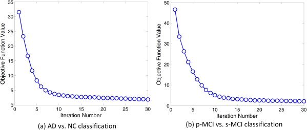
Objective function values versus optimization iteration number in (a) AD versus NC classification and (b) p‐MCI versus s‐MCI classification. [Color figure can be viewed in the online issue, which is available at http://wileyonlinelibrary.com.]
Ensemble Classification
After obtaining K feature subsets using our proposed view‐centralized feature selection algorithm, we can then learn K base classifiers individually. In this study, a linear SVM classifier is used to identify AD patients from NCs, and progressive MCI patients from stable MCI patients. Here, we choose a linear model because it has good generalization capability across different training data as shown in extensive studies [Burges, 1998; Pereira et al., 2009; Zhang and Shen, 2012]. Finally, a classifier ensemble strategy is used to combine these K base classifiers to construct a more accurate and robust learning model. Among various classifier combination approaches, we use the majority voting strategy because it is very simple and is one of the more widely used methods for the fusion of multiple classifiers. Thus, the class label of an unseen test sample can be determined by majority voting for the outputs of K base classifiers.
Implementation Details
In this study, we adopt a 10‐fold cross‐validation strategy to evaluate the performance of our proposed method. To be specific, all subject samples are partitioned into 10 subsets (each subset with a roughly equal size), and each time all samples within one subset are successively selected as the testing data, while the remaining samples in the other nine subsets are combined together as the training data to perform feature selection and classification. Finally, we report the average values of classification results across all 10 cross‐validation folds. It is worth noting that the 10‐fold cross‐validation strategy has been widely used in recent neuroimaging based classification [Jie et al., 2014; Liu et al., 2014; Min et al., 2014b; Zhang and Shen, 2012].
In our proposed feature selection algorithm, the regularization parameters and are chosen from {2−10, 2−9, , 20} through cross‐validation on the training data. More specifically, in each fold of the 10‐fold cross validation, we further split the training set into the training part and the validation part. By varying the values of both and in the proposed feature selection method, we can obtain different feature subsets based on samples in the training part, and record the classification results on the validation data. The values of and with the best classification accuracy on the validation data will then be chosen. Here, the linear SVM [Chang and Lin, 2011] is used as the classifier, with the default value for the parameter C (i.e., C = 1). Similarly, the parameter for the L1‐norm regularization term in Lasso is selected from {2−10, 2−9, , 20} through cross‐validation on the training data. In addition, the weighting value for the main‐view group is set as 0.1, and the weighting value for the side‐view group is set as 0.9 empirically, because with such settings we can not only concentrate on one main atlas but also make full use of information provided by other atlases. In the Results section, we will further investigate the influence of parameters on the performance of our proposed method.
In our experiments, we use four measurement criteria to evaluate the performances of different methods, including classification accuracy (ACC), classification sensitivity (SEN), classification specificity (SPE), and the area under the receiver operating characteristic (ROC) curve (AUC). To be specific, the accuracy measures the proportion of subjects that are correctly predicted among all studied subjects, the sensitivity denotes the proportion of AD patients (or p‐MCI) that are correctly predicted, and the specificity represents the proportion of NC (or s‐MCI) that are correctly predicted.
To evaluate the efficacy of our proposed method, we perform experiments on part of subjects in the ADNI database (http://adni.loni.usc.edu/). The ADNI database was launched in 2003 by the National Institute on Aging (NIA), the National Institute of Biomedical Imaging and Bioengineering (NIBIB), the Food and Drug Administration (FDA), private pharmaceutical companies and nonprofit organizations, as a $60 million, 5‐year public–private partnership. The primary goal of the ADNI has been to test whether different biological markers (e.g., such as magnetic resonance imaging (MRI) and Positron Emission Tomography (PET)) as well as clinical and neuropsychological assessment can be combined to measure the progression of MCI and early AD. Determination of sensitive and specific markers of very early AD progression is intended to aid researchers and clinicians to develop new treatments and monitor their effectiveness, as well as lessen the time and the cost of clinical trials. The Principal Investigator of this initiative is Michael W. Weiner MD, VA Medical Center and University of California, San Francisco. The ADNI was the result of efforts of many coinvestigators from a broad range of academic institutions and private corporations. The studied subjects were recruited from over 50 sites across the U.S. and Canada, and gave written informed consent at the time of enrollment for imaging and genetic sample collection, as well as completed questionnaires approved by each of the participating sites' Institutional Review Board (IRB).
In this study, we use T1‐weighted MRI data in ADNI‐1 [Jack et al., 2008] for AD‐related disease diagnosis. In our experiments, there are a total of 459 subjects, randomly selected from those scanned with a 1.5T scanner, including 97 AD, 128 NC, and 234 MCI (117 p‐MCI and 117 s‐MCI) subjects. The scanning parameters for the 1.5T MRI data used in this study can be found from [Jack et al., 2008]. It is worth noting that not all subjects with MRI data from the ADNI‐1 database are used, because it requires much preprocessing time to register all subjects to multiple atlases (i.e., 10 atlases in this study). Conversely, the subject size used in our experiments is very similar to that used in many previous studies [Cuingnet et al., 2011; Koikkalainen et al., 2011; Liu et al., 2014; Min et al., 2014a; Zhang et al., 2011], and is sufficient to compare the proposed method with the other methods. The demographic information of the studied subjects is shown in Table 1.
Table 1.
Demographic information of the studied subjects from ADNI database
| Diagnosis | Number | Age | Gender (M/F) | MMSE |
|---|---|---|---|---|
| AD | 97 | 75.90 ± 6.84 | 48/49 | 23.37 ± 1.84 |
| NC | 128 | 76.11 ± 5.10 | 63/65 | 29.13 ± 0.96 |
| p‐MCI | 117 | 75.18 ± 6.97 | 67/50 | 26.45 ± 1.66 |
| s‐MCI | 117 | 75.09 ± 7.65 | 79/38 | 27.42 ± 1.78 |
Values are denoted as mean ± deviation; MMSE means mini‐mental state examination; M and F represent male and female, respectively.
RESULTS
AD Classification
Classification using single atlases
To demonstrate the variability of classification results using different atlases, we first report the results of AD versus NC classification based on a single atlas. Note that, in the single atlas case, our proposed VCMA feature selection method uses only features from a particular atlas (i.e., main view), while features from other atlases are completely ignored (i.e., and ); thus Eq. (1) is similar to the formulation of elastic net [Zou and Hastie, 2005]. In this group of experiments, we compare our method with two conventional feature selection methods. The first one is based on the ranking of PC coefficients, and the second one is the COMPARE method proposed in [Fan et al., 2007] that combines PC and SVM‐RFE [Guyon et al., 2002]. For fair comparison, the linear SVM with default parameter (C = 1) is adopted as a classifier after feature selection using PC, COMPARE, and our proposed method. In Figure 5, we report the distribution of classification results achieved by PC, COMPARE, and our method using 10 single atlases in AD versus NC classification.
Figure 5.
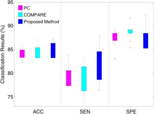
Distribution of accuracy (ACC), sensitivity (SEN) and specificity (SPE) achieved by different singleatlas based methods in AD versus NC classification. [Color figure can be viewed in the online issue, which is available at http://wileyonlinelibrary.com.]
As can be seen in Figure 5, the classification results using different single atlases are very different, regardless of the use of different feature selection methods. The underlying reason may be that the anatomical structure of a certain atlas may be more representative for the entire population, compared with other atlases. In this case, the overall registration errors of this atlas are smaller and, thus, the feature representation generated from this atlas includes less noise. Another possible reason could be that the AD‐related patterns generated from a certain atlas may be more discriminative than those generated from other atlases, thus, have better generalization capability in identifying unseen test subjects. Conversely, from Figure 5, one can see that the overall performance of our proposed method is better than that of PC and that of COMPARE, in terms of classification accuracy and sensitivity. Especially, our method achieves the best sensitivity among the three compared methods, indicating that our method can effectively classify AD patients from the NCs. Although COMPARE achieves the best specificity, its accuracy and sensitivity are lower than our method.
Classification using multiple atlases
In this subsection, we show results for AD versus NC classification using multiple atlases. Here, we compare our method with six feature selection methods, including (1) single‐atlas based PC (PC_SA); (2) single‐atlas based COMPARE (COMPARE_SA); (3) multiple‐atlas based PC (PC_MA); (4) multiple‐atlas based COMPARE (COMPARE_MA); (5) Random subspace (RS) [Ho, 1998] that randomly selects features from the original feature space; and (6) Lasso [Tibshirani, 1996] that is a widely used feature selection method in neuroimaging analysis. Specifically, we report the averaged classification results of single‐atlas based methods (i.e., PC and COMPARE) among all 10 atlases for PC_SA and COMPARE_SA, respectively. It is worth noting that all compared methods use the same feature representation (i.e., 15,000‐dimensional) generated from 10 atlases. Similar to the work in [Min et al., 2014a], for both PC_MA and COMPARE_MA methods, we first concatenate all regional features (i.e., 15,000‐dimensional) extracted from multiple atlases. Then, the top M (M = ) features are sequentially selected according to the PC (with respect to class labels) for PC_MA and PC+SVM‐RFE for COMPARE_MA, and the best classification results are reported. It is worth noting that, in our proposed method, we learn 10 SVM classifiers based on different atlas‐centralized feature subsets determined by our proposed feature selection method, and then construct a classifier ensemble with these learned base classifiers. For fair comparison, for the RS method, we randomly select M (M = ) features from each atlas for classification, and then record the best result. For the Lasso method, we first learn a Lasso model based on the features from one specific atlas, and then select features with non‐zero coefficient in the learned weight vector. Given 10 atlases, 10 classifiers can be constructed based on the features selected by RS and Lasso, respectively. Finally, for the RS and Lasso methods, these classifiers are combined by the same ensemble strategy as used in our proposed method. The experimental results are summarized in Table 2, and Figure 6 shows the ROC curves achieved by the different methods.
Table 2.
Results of AD versus NC classification using single atlas and multiple atlases
| Method | ACC (%) | SEN (%) | SPE (%) | AUC |
|---|---|---|---|---|
| PC_SA | 84.00 | 79.53 | 87.45 | 0.7692 |
| COMPARE_SA | 84.18 | 75.33 | 89.17 | 0.7870 |
| PC_MA | 85.91 | 81.56 | 89.23 | 0.8191 |
| COMPARE_MA | 87.19 | 80.56 | 92.31 | 0.8495 |
| RS | 85.44 | 69.00 | 92.75 | 0.7688 |
| Lasso | 87.27 | 84.78 | 89.23 | 0.9004 |
| Proposed method | 92.51 | 92.89 | 88.33 | 0.9583 |
PC_SA and COMPARE_SA denote PC and COMPARE using single atlas, respectively; PC_MA and COMPARE_MA mean PC and COMPARE using multiple atlases, respectively; RS represents random subspace; ACC denotes accuracy; SEN means sensitivity; SPE represents specificity, and AUC denotes the area under ROC curve.
Figure 6.
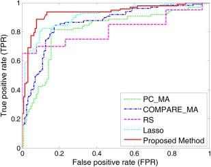
ROC curves for the classification between AD and NC achieved by different methods. [Color figure can be viewed in the online issue, which is available at http://wileyonlinelibrary.com.]
From Table 2 and Figure 6, it is clear to see that multiatlas based methods (i.e., PC_MA, COMPARE_MA, RS, Lasso, and our proposed method) generally achieve much better performance than single‐atlas based methods (i.e., PC_SA and COMPARE_SA). Specifically, the best accuracies achieved by PC_SA and COMPARE_SA are only 84.00% and 84.18%, respectively, which are much lower than those of COMPARE_MA, Lasso, and our proposed method. This demonstrates that, compared with the case of using single atlas, using multiple atlases can improve the performance of AD classification, which is consistent with the conclusion in [Min et al., 2014a, 2014b]. Conversely, Table 2 shows that our proposed method consistently outperforms other methods in terms of classification accuracy, sensitivity, and AUC value. To be specific, our method achieves a classification accuracy of 92.51%, a sensitivity of 92.89%, and an AUC of 0.9583, while, among the other methods, the best accuracy is 87.27%, the best sensitivity is 84.78%, and the best AUC is 0.9004. Obviously, by focusing on the representation from a certain atlas with other atlases as extra guidance, our method achieves better performance than the compared methods.
In addition, from Table 2, we can observe that the sensitivities of PC_SA, COMPARE_SA, PC_MA, COMPARE_MA, RS, and Lasso are much lower than their corresponding specificities. Here, low sensitivity values indicate low confidence in AD diagnosis, which will greatly limit the practical usage in real‐world applications. In contrast, our method achieves a significantly improved sensitivity value (i.e., nearly 8% higher than the second best sensitivity achieved by Lasso). This characteristic of possessing a high sensitivity may be advantageous for a confident AD diagnosis, which is potentially very useful in practice.
MCI Conversion Prediction
Prediction using single atlases
Similar to the AD versus NC classification experiments, we evaluate single‐atlas based methods in MCI conversion prediction (i.e., p‐MCI vs. s‐MCI classification), with results reported in Figure 7. From Figure 7, one can see that using different single atlases yields a large variation of classification results, which is similar to the trend in AD versus NC classification. In addition, as shown in Figure 7, our method generally achieves much better results than PC and COMPARE in terms of the classification accuracy, sensitivity, and specificity. Conversely, from Figures 5 and 7, one can see that the results of p‐MCI versus s‐MCI classification are much lower than those of AD versus NC classification. The reason may be that MCI can be regarded as the early stage of AD, where the related atrophy is small and not as discriminative in distinguishing p‐MCI from s‐MCI subjects [Jie et al., 2014; Suk et al., in press].
Figure 7.
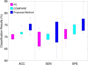
Distributions of accuracy (ACC), sensitivity (SEN) and specificity (SPE) achieved by different singleatlas based methods in p‐MCI versus s‐MCI classification. [Color figure can be viewed in the online issue, which is available at http://wileyonlinelibrary.com.]
Prediction using multiple atlases
In this subsection, we perform p‐MCI versus s‐MCI classification using feature representations generated from multiple atlases. The experimental results are reported in Table 3. We further plot the ROC curves achieved by different methods in Figure 8.
Table 3.
Results of p‐MCI versus s‐MCI classification using single atlas and multiple atlases
| Method | ACC (%) | SEN (%) | SPE (%) | AUC |
|---|---|---|---|---|
| PC_SA | 68.49 | 67.80 | 69.10 | 0.6285 |
| COMPARE_SA | 70.06 | 68.08 | 72.02 | 0.6356 |
| PC_MA | 72.78 | 74.62 | 70.91 | 0.7245 |
| COMPARE_MA | 73.35 | 75.76 | 70.83 | 0.7405 |
| RS | 69.05 | 68.10 | 72.94 | 0.6912 |
| Lasso | 75.32 | 81.36 | 69.17 | 0.7602 |
| Proposed method | 78.88 | 85.45 | 76.06 | 0.8069 |
Note: PC_SA and COMPARE_SA denote PC and COMPARE using single atlas, respectively; PC_MA and COMPARE_MA mean PC and COMPARE using multiple atlases, respectively; RS represents random subspace; ACC denotes accuracy; SEN means sensitivity; SPE represents specificity, and AUC denotes the area under ROC curve.
Figure 8.
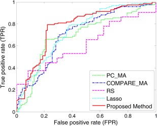
ROC curves for the classification between p‐MCI and s‐MCI achieved by different methods. [Color figure can be viewed in the online issue, which is available at http://wileyonlinelibrary.com.]
From Table 3 and Figure 8, we can observe again that multiatlas based methods generally outperform single‐atlas based ones. For example, the best accuracy of multiatlas based methods (achieved by our method) is 78.88%, which is significantly better than the best accuracy of single‐atlas based methods, that is, 70.06% (achieved by COMPARE_SA). In addition, among the five multiatlas based methods, our proposed method achieves consistently better performances than the other four methods in terms of classification accuracy, sensitivity, specificity, and AUC value. Especially, our proposed method achieves an area under the ROC curve (AUC) of 0.8069, while the best AUC value of the compared methods is only 0.7602 (achieved by Lasso). Furthermore, Table 2 and Table 3 also indicate that, for both AD versus NC classification and p‐MCI versus s‐MCI classification, our proposed method achieves much higher sensitivities than the compared methods, implying that our method can produce more confident diagnosis results for both AD and progressive MCI patients.
Comparison with Existing Classification Methods
In this subsection, we compare the results achieved by our proposed method with some recent results reported in the literature, which are also based on the MRI data of ADNI subjects for AD/MCI classification. To be specific, we compare our method with seven methods, which are based on either single atlas [Cuingnet et al., 2011; Liu et al., 2012, 2014; Zhang et al., 2011] or multiple atlases [Koikkalainen et al., 2011; Min et al., 2014a, 2014b]. For fair comparison, results using only MRI data are reported for the multimodality based approach in [Zhang et al., 2011]. In Tables 4 and V, we report the results of AD versus NC classification and p‐MCI versus s‐MCI classification, respectively. In addition, we further list the details of each method in Tables 4 and V, including the type of features, classifiers, and subjects used in the corresponding methods.
Table 4.
Comparison of AD versus NC classification results reported in the literature using MR imaging data of ADNI subjects
| Method | Feature | Classifier | Subjects | Atlas | ACC (%) | SEN (%) | SPE (%) |
|---|---|---|---|---|---|---|---|
| Cuingnet et al. [2011] | Voxel‐Direct‐D GM | SVM | 137 AD + 162 NC | Single‐atlas | 88.58 | 81.00 | 95.00 |
| Zhang et al. [2011] | 93 ROI GM | SVM | 51 AD + 52 NC | Single‐atlas | 86.20 | 86.00 | 86.30 |
| Liu et al. [2012] | Voxel‐Wise GM | SRC ensemble | 198 AD + 229 NC | Single‐atlas | 90.80 | 86.32 | 94.76 |
| Liu et al. [2014] | Patch‐Based GM | SVM ensemble | 198 AD + 229 NC | Single‐atlas | 92.00 | 91.00 | 93.00 |
| Koikkalainen et al. [2011] | Tensor‐Based Morphometry | Linear regression | 88 AD + 115 NC | Multi‐atlas | 86.00 | 81.00 | 91.00 |
| Min et al. [2014a] | Data‐Driven ROI GM | SVM | 97 AD + 128 NC | Multi‐atlas | 91.64 | 88.56 | 93.85 |
| Min et al. [2014b] | Data‐Driven ROI GM | SVM | 97 AD + 128 NC | Multi‐atlas | 90.69 | 87.56 | 93.01 |
| Proposed method | Data‐Driven ROI GM | SVM ensemble | 97 AD + 128 NC | Multi‐atlas | 92.51 | 92.89 | 88.33 |
ACC denotes accuracy, SEN means sensitivity, and SPE represents specificity.
As shown in Table 4, for AD versus NC classification, our proposed method is superior to the compared methods, in terms of both classification accuracy and sensitivity. More specifically, our method achieves an accuracy of 92.51% and a sensitivity of 92.89%, while only the method proposed in [Liu et al., 2014] obtained comparable results, with an accuracy of 92.00% and a sensitivity of 91.00%. Although researchers in [Cuingnet et al., 2011] reported the highest specificity value, their accuracy and sensitivity are relatively lower than our method. Conversely, among the four multiatlas based methods, our proposed method achieves significantly higher accuracy and sensitivity than the method proposed in [Koikkalainen et al., 2011] which simply averaged feature representations from different atlases. At the same time, our method obtains slightly better accuracy, but much higher sensitivity, than methods proposed in [Min et al., 2014a, 2014b], which simply concatenated feature representations from multiple atlases.
Among all compared methods, only four methods (i.e., those in [Cuingnet et al., 2011; Koikkalainen et al., 2011; Min et al., 2014a, 2014b]) report their results of p‐MCI versus s‐MCI classification, which is a more difficult classification task. Accordingly, we list their performances as well as ours in Table 5. In the work of [Cuingnet et al., 2011], the best results for AD versus NC classification and p‐MCI versus s‐MCI classification were obtained using different features. That is, they used the GM tissue density map for AD versus NC classification, and adopted a subset of features selected by the method proposed in [Vemuri et al., 2008] for p‐MCI versus s‐MCI classification. In addition, the best results in [Koikkalainen et al., 2011] are obtained by combing the classifiers trained from different atlases, which is different from the strategy used in AD versus NC classification. In [Min et al., 2014a], the best result of p‐MCI versus s‐MCI classification is obtained in a transfer‐learning manner. That is, they use the abnormal patterns identified between AD and NC for guiding p‐MCI versus s‐MCI classification. In addition, the best result reported in [Min et al., 2014b] is based on a new representation learned from the feature concatenation of multiple representations generated from multiple atlases.
Table 5.
Comparison of p‐MCI versus s‐MCI classification results reported in the literature using MR imaging data of ADNI subjects
| Method | Feature | Classifier | Subjects | Atlas | ACC (%) | SEN (%) | SPE (%) |
|---|---|---|---|---|---|---|---|
| Cuingnet et al. [2011] | Voxel‐stand‐D GM | SVM | 76 p‐MCI + 134 s‐MCI | Single‐atlas | 70.40 | 57.00 | 78.00 |
| Koikkalainen et al. [2011] | Tensor‐based Morphometry | Linear regression | 54 p‐MCI + 115 s‐MCI | Multi‐atlas | 72.10 | 77.00 | 71.00 |
| Min et al. [2014a] | Data‐driven ROI GM | SVM | 117 p‐MCI + 117 s‐MCI | Multi‐atlas | 72.41 | 72.12 | 72.58 |
| Min et al. [2014b] | Data‐driven ROI GM | SVM | 117 p‐MCI + 117 s‐MCI | Multi‐atlas | 73.69 | 76.44 | 70.76 |
| Proposed method | Data‐driven ROI GM | SVM ensemble | 117 p‐MCI + 117 s‐MCI | Multi‐atlas | 78.88 | 85.45 | 76.06 |
ACC denotes accuracy, SEN means sensitivity, and SPE represents specificity.
From Table 5, we can observe that our proposed method achieves much higher classification accuracy and sensitivity than the other four methods. Specifically, our method achieves a classification accuracy of 78.88% and a sensitivity of 85.45%, while the best accuracy and the best sensitivity obtained by the compared methods are only 73.69% and 77.00%, respectively. Although the specificity reported in [Cuingnet et al., 2011] is higher than those of other methods, its accuracy and sensitivity are much lower than our method.
DISCUSSION
Effect of Atlas Number
In this subsection, we investigate the effect of different atlas numbers on the performance of our proposed method. By adding more atlases, we report the classification accuracy achieved by our method in AD versus NC classification and p‐MCI versus s‐MCI classification in Figure 9. As shown in Figure 9, in both AD versus NC and p‐MCI versus s‐MCI classification tasks, the accuracy achieved by our method rises gradually with the increase of atlas number. To demonstrate the underlying reason, we further analyze the correlation relationship among multiple atlases used in this study.
Figure 9.
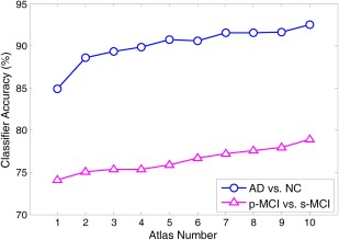
Results of our proposed method by adding the atlas number from 1 to 10 in both the AD versus NC classification (a line with circle markers) and the p‐MCI versus s‐MCI classification (a line with triangle markers). [Color figure can be viewed in the online issue, which is available at http://wileyonlinelibrary.com.]
As different atlases generally have different anatomical structures, features from different atlases may be extracted from different ROIs in the feature extraction stage. In such case, it could be meaningless to directly compute correlation between feature representations from two atlases. To model correlation relationship among multiple atlases, we will first define the correlation coefficient between two atlases. Let and denote the feature dimension in two atlas (i.e., and ) spaces ( in this study), respectively. Denote as the correlation coefficient between two atlases and , and can be computed in the following way:
| (7) |
where denotes the pth feature vector on the training samples in the atlas , denotes the qth feature vector on the training samples in the atlas , and represents the PC coefficient between and . Note that , and a larger value of denotes that the atlas and the atlas tend to be more correlated. Based on the definition in Eq. (7), we plot the correlation coefficients among 10 atlases (i.e., to ) in Figure 10.
Figure 10.
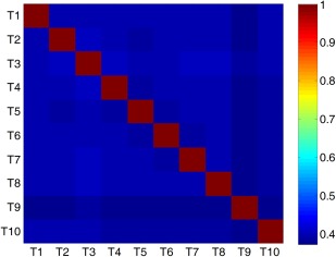
Correlation coefficients among ten atlases computed according to Eq. (7). Here, red and yellow indicate high correlation coefficients, while blue and green denote low coefficients. [Color figure can be viewed in the online issue, which is available at http://wileyonlinelibrary.com.]
As can be seen from Figure 10, these atlases are not highly correlated, with relatively low pairwise correlation coefficients. For example, the correlation coefficients of atlas T9 and other atlases are consistently smaller than 0.5. Conversely, results in Figures 9 and 10 imply that, if multiple atlases are not highly relevant, using features from more atlases tends to help improve the classification result. This could partly explain why increasing the number of atlases can boost the classification performance of our method.
Analysis of Diversity
To understand how our ensemble approach works, we use the kappa measure to plot the diversity‐error diagram, which evaluates the level of agreement between the outputs of two classifiers [Rodriguez et al., 2006]. In Figure 11, we show the diversity‐error diagrams of RS, Lasso, and our proposed method in AD versus NC classification and p‐MCI versus s‐MCI classification tasks. For each method, the corresponding ensemble contains 10 individual classifiers that correspond to 10 different atlases. The value on the x‐axis of a diversity‐error diagram denotes the kappa diversity of a pair of classifiers in the ensemble, while the value on the y‐axis is the averaged individual error of a pair of classifiers. As a small value of kappa diversity indicates better diversity and a small value of averaged individual error indicates a better accuracy, the most desirable pairs of classifiers will be close to the bottom left corner of the graph. It is worth noting that, as shown in Figure 11a, there are a small number of points for RS and our method in AD versus NC classification, because many classifier pairs have the same diversity and classification errors. For visual evaluation of the relative positions of the clouds of Kappa‐error points, we also plot the centroids of clouds for three methods in Figure 11.
Figure 11.
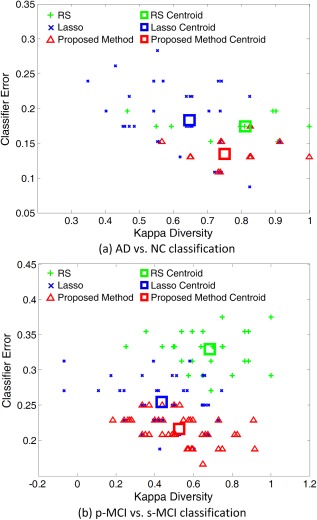
The diversity‐error diagrams of classifiers in (a) AD versus NC classification and (b) p‐MCI versus s‐MCI classification using RS, Lasso and our proposed method. The final ensemble is composed of ten classifiers. The x‐axis represents the diversity of a pair of classifiers evaluated by the kappa measure, and y‐axis represents the average classification error of a pair of classifiers. The green, blue and red squares denote the centroids of RS, Lasso, and our proposed method classifier clouds, respectively. [Color figure can be viewed in the online issue, which is available at http://wileyonlinelibrary.com.]
From Figure 11a,b, we can observe that, in both AD versus NC classification and p‐MCI versus s‐MCI classification, our proposed method achieves much higher diversity as well as many fewer errors than those of RS. At the same time, our proposed method is not as diverse as Lasso, but apparently, it has more accurate base classifiers than Lasso. As shown in Tables 2 and III, our proposed method outperforms Lasso in both AD versus NC and p‐MCI versus s‐MCI classification tasks. It seems that our proposed method can achieve a better trade‐off between accuracy and diversity than the compared methods. That is, it builds a classifier ensemble based on the reasonably diverse but markedly accurate individual components [Rodriguez et al., 2006].
Effect of Parameters
In this subsection, we evaluate the influence of parameters on the performance of our proposed method. In the experiments, we vary the values of and in the range of {2−10, 2−9, , 20}, and record the corresponding classification results achieved by our method in AD versus NC classification. The experimental results are shown in Figure 12. From Figure 12a,b, we can clearly see that the classification accuracy and sensitivity slightly fluctuate in a small range with the increase of and . At the same time, Figure 12c,d reveal that the specificity and AUC value achieved by our method are generally stable with respect to these two parameters (i.e., and ).
Figure 12.
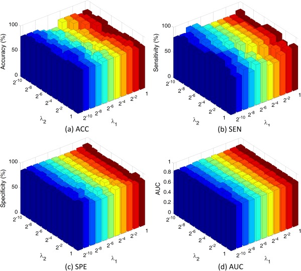
Results of AD versus NC classification with different parameter values for λ1 and λ2. Note that λ1 and λ2 are chosen from {2−10, 2−9, ⋯, 20}. Here, ACC denotes accuracy, SEN means sensitivity, SPE represents specificity, and AUC denotes the area under ROC curve. [Color figure can be viewed in the online issue, which is available at http://wileyonlinelibrary.com.]
Furthermore, we investigate the influence of different weighting values for the main‐view group (i.e., ) and the side‐view group (i.e., ) on the performance of our proposed method. In this group of experiments, we gradually increase the value of (where ), and record the corresponding classification results achieved by our method. The classification results versus different weighting values for the main‐view group (i.e., ) in AD versus NC classification and p‐MCI versus s‐MCI classification are shown in Figure 13.
Figure 13.
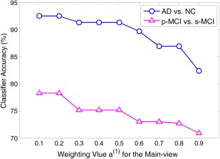
Classification accuracy achieved by our proposed method with different weighting values of a(1) for the main‐view group in AD versus NC classification (a line with circle markers) and p‐MCI versus s‐MCI classification (a line with triangle markers). Note that the weighting values for the main‐view group range from 0.1 to 0.9 with step 0.1, while other two parameters λ1 and λ2 are chosen from {2−10, 2−9, ⋯, 20} through cross‐validation. [Color figure can be viewed in the online issue, which is available at http://wileyonlinelibrary.com.]
As shown in Figure 13, in both classification tasks, the accuracy obtained by our proposed method gradually becomes worse with the increase of the weighting value for the main‐view (i.e., ) in a large scale. For example, in AD versus NC classification, our method achieves higher classification accuracy when the value of is smaller than 0.3, and achieves the worst performance with (i.e., ). In p‐MCI versus s‐MCI classification, we can find the similar trend as in AD versus NC classification. It is worth noting that, in our proposed method, a small value of (as well as a large value of ) indicates that more features are selected from the main‐view group (i.e., main atlas), while relatively less features are selected from the side‐view group (i.e., supplementary atlases). The results in Figure 13 imply that focusing on a certain atlas, along with extra guidance from other atlases (as done in our proposed method), can offer more accurate diagnosis results.
Clinical Relevance and Limitations
This study proposes a novel VCMA classification method for AD diagnosis. Compared with the conventional ways of simple feature concatenation and averaging, our method provides a unified way to combine features generated from multiple atlases. Experimental results on 459 subjects from ADNI database demonstrate that our method can consistently and substantially outperform the existing multiatlas based classification methods. Specifically, our method can achieve high accuracies of 92.51% and 78.88% for AD versus NC classification and p‐MCI versus s‐MCI classification, respectively. It is worth noting that our method is general for various disease diagnosis applications where multiview (or multimodality) features can be obtained.
In recent studies, several works have shown that feature representations from multiple atlases may contain complementary information for AD diagnosis [Cuingnet et al., 2011; Koikkalainen et al., 2011; Min et al., 2014a, 2014b; Wolz et al., 2011]. However, most existing studies simply average or concatenate these multiple feature representations, thus ignore potentially important diagnosis information related to the anatomical differences of individual atlases. Conversely, as features are extracted from multiple atlases, they could be redundant, which increases the difficluty for the subsequent learning process. As an effective way to eliminate such redundant features, feature selection is commonly used for identifying discriminative biomarkers for AD and MCI. For example, researchers in [Min et al., 2014a] proposed a correlation‐and‐relevance‐based feature selection method using the concatenation of features from multiple atlases, and thus ignores the redundancy of complementary information conveyed in multiatlas data. To this end, we propose a VCMA feature selection method, where each time we focus only on one atlas with the extra guidance from other atlases. The good classification results achieved by our method indicate its good diagnostic power. As can be seen from Tables 2 and III, our method achieves superior performance over the compared methods.
In this study, we also propose an ensemble classification method by combining the results of multiple classifiers corresponding to multiple atlases. As can be seen from Tables 2 and III, the methods using ensemble strategy (including PC, Lasso, and our proposed method) often perform better than other methods, demonstrating the effectiveness of the ensemble strategy in boosting the classification results based on multiatlas data. In Figure 11, we plot the diversity‐error diagram to understand how our ensemble approach works. It can be seen that our proposed method achieves a better trade‐off between accuracy and diversity than the compared methods in both AD versus NC and p‐MCI versus s‐MCI classification tasks.
Furthermore, in Tables 4 and V, we compare our method with the recent state‐of‐the‐art methods for MRI‐based AD/MCI classification. It is clear that our method achieves the best classification accuracy and sensitivity. To investigate the influence of parameters on the performance of our method, we further perform experiments by varying the parameter values (i.e., and ) and record their corresponding results, as shown in Figure 12. We can see that our method is not sensitive to the selection of parameter values. In addition, we study the influence of the weighting value for the main view (i.e., ), with experimental results given in Figure 13. It can be seen that focusing on a certain atlas (along with the extra guidance from other atlases) can offer more accurate diagnosis results.
However, this study is limited by the following factors. First, our method has high computational cost due to the use of multiple atlases for image registration. Second, only the regional features are extracted for feature representation, while other morphometric features such as Jacobian determinants can also be used in our method. Third, we only use MRI data to learn the classification model, although there are other types of biomarkers, such as fluorodeoxyglucose positron emission tomography (FDG‐PET). Specifically, the use of multiple biomarkers can potentially further boost the learning performance of our method, as confirmed in many recent works [Zhang and Shen, 2012; Zhang et al., 2011]. Finally, we only use the MRI baseline data in ADNI in our experiments. In the future, we will use both baseline data and longitudinal data to characterize the spatiotemporal development pattern of brain atrophy for better diagnosis and prediction of brain disease. For example, the longitudinal changing patterns can be captured using multiple atlases, and thus the longitudinal features from different atlases can be used as multiview features for classification with our proposed view‐centralized classification method. All these will be our future work for further improving the diagnosis performance with new features, multimodality data, and longitudinal images.
CONCLUSION
In this study, we propose a novel VCMA classification method, which can better exploit the useful information in different feature representations from multiple atlases. Specifically, we first register all brain images onto multiple atlases individually, for extracting the respective feature representation in each atlas space. Then, we apply the proposed view‐centralized multi‐atlas feature selection method to select the most discriminative features corresponding to each atlas, using other atlases as extra guidance. Finally, for each atlas, we learn a SVM classifier using the selected features specific to each atlas, and further combine multiple SVM classifiers corresponding to multiple atlases through a classifier ensemble strategy for making a final decision. Experimental results on 459 subjects from the ADNI database have demonstrated significant performance improvement for both AD versus NC classification and p‐MCI versus s‐MCI classification. In the current study, we evaluate the proposed method on AD/MCI classification. Actually, our method can also be used in other brain analysis applications, such as autism and schizophrenia diagnosis, which will be our future work.
ACKNOWLEDGMENTS
The authors would like to thank editor and anonymous reviewers for their constructive comments and contributions for the improvement of this article.
Data used in preparation of this article were obtained from the Alzheimer's Disease Neuroimaging Initiative (ADNI) database (http://www.loni.ucla.edu/ADNI). As such, the investigators within the ADNI contributed to the design and implementation of ADNI and/or provided data but did not participate in analysis or writing of this report. A complete listing of ADNI investigators can be found at http://www.loni.ucla.edu/ADNI/Collaboration/ADNI_Authorship_list.pdf .
REFERENCES
- Ashburner J, Friston KJ (2000): Voxel‐based morphometry‐the methods. NeuroImage 11:805–821. [DOI] [PubMed] [Google Scholar]
- Ashburner J, Hutton C, Frackowiak R, Johnsrude I, Price C, Friston K (1998): Identifying global anatomical differences: Deformation‐based morphometry. Hum Brain Mapp 6:348–357. [DOI] [PMC free article] [PubMed] [Google Scholar]
- Basha T, Moses Y, Kiryati N (2013): Multi‐view scene flow estimation: A view centered variational approach. Int J Comput Vis 101:6–21. [Google Scholar]
- Beck A, Teboulle M (2009): A fast iterative shrinkage‐thresholding algorithm for linear inverse problems. Siam J Imging Sci 2:183–202. [Google Scholar]
- Bozzali M, Filippi M, Magnani G, Cercignani M, Franceschi M, Schiatti E, Castiglioni S, Mossini R, Falautano M, Scotti, G , Comi G, Falini A. (2006): The contribution of voxel‐based morphometry in staging patients with mild cognitive impairment. Neurology 67:453–460. [DOI] [PubMed] [Google Scholar]
- Brookmeyer R, Johnson E, Ziegler‐Graham K, Arrighi HM (2007): Forecasting the global burden of Alzheimer's disease. Alzheimers Dement 3:186–191. [DOI] [PubMed] [Google Scholar]
- Burges CJ (1998): A tutorial on support vector machines for pattern recognition. Data Min Knowl Disc 2:121–167. [Google Scholar]
- Chan D, Janssen JC, Whitwell JL, Watt HC, Jenkins R, Frost C, Rossor MN, Fox NC (2003): Change in rates of cerebral atrophy over time in early‐onset Alzheimer's disease: Longitudinal MRI study. Lancet 362:1121–1122. [DOI] [PubMed] [Google Scholar]
- Chang C‐C, Lin C‐J(2011): LIBSVM: A library for support vector machines. ACM Trans Intell Syst Technol 2:27. [Google Scholar]
- Chen X, Pan W, Kwok JT, Carbonell JG (2009a): Accelerated gradient method for multitask sparse learning problem. In Proceedings of IEEE International Conference on Data Mining. Florida, USA.
- Chen Y, An H, Zhu H, Stone T, Smith JK, Hall C, Bullitt E, Shen D, Lin W (2009b): White matter abnormalities revealed by diffusion tensor imaging in non‐demented and demented HIV+ patients. NeuroImage 47:1154–1162. [DOI] [PMC free article] [PubMed] [Google Scholar]
- Chung M, Worsley K, Paus T, Cherif C, Collins D, Giedd J, Rapoport J, Evans A (2001): A unified statistical approach to deformation‐based morphometry. NeuroImage 14:595–606. [DOI] [PubMed] [Google Scholar]
- Cuingnet R, Gerardin E, Tessieras J, Auzias G, Lehéricy S, Habert, M.‐O. , Chupin M, Benali H, Colliot O (2011): Automatic classification of patients with Alzheimer's disease from structural MRI: A comparison of ten methods using the ADNI database. NeuroImage 56:766–781. [DOI] [PubMed] [Google Scholar]
- Davatzikos C, Genc A, Xu D, Resnick SM (2001): Voxel‐based morphometry using the RAVENS maps: Methods and validation using simulated longitudinal atrophy. NeuroImage 14:1361–1369. [DOI] [PubMed] [Google Scholar]
- Davatzikos C, Fan Y, Wu X, Shen D, Resnick SM (2008): Detection of prodromal Alzheimer's disease via pattern classification of magnetic resonance imaging. Neurobiol Aging 29:514–523. [DOI] [PMC free article] [PubMed] [Google Scholar]
- Dennis JJE, Schnabel RB (1983): Numerical Methods for Unconstrained Optimization and Nonlinear Equations. Prentice‐Hall, Inc, Englewood Cliffs, NJ. [Google Scholar]
- Dickerson BC, Goncharova I, Sullivan M, Forchetti C, Wilson R, Bennett D, Beckett L, deToledo‐Morrell L (2001): MRI‐derived entorhinal and hippocampal atrophy in incipient and very mild Alzheimer's disease. Neurobiol Aging 22:747–754. [DOI] [PubMed] [Google Scholar]
- Fan Y, Shen D, Gur RC, Gur RE, Davatzikos C (2007): COMPARE: Classification of morphological patterns using adaptive regional elements. IEEE Trans Med Imaging 26:93–105. [DOI] [PubMed] [Google Scholar]
- Fan Y, Resnick SM, Wu X, Davatzikos C (2008): Structural and functional biomarkers of prodromal Alzheimer's disease: A high‐dimensional pattern classification study. NeuroImage 41:277–285. [DOI] [PMC free article] [PubMed] [Google Scholar]
- Fox N, Warrington E, Freeborough P, Hartikainen P, Kennedy A, Stevens J, Rossor MN (1996): Presymptomatic hippocampal atrophy in Alzheimer's disease A longitudinal MRI study. Brain 119:2001–2007. [DOI] [PubMed] [Google Scholar]
- Frey BJ, Dueck D (2007): Clustering by passing messages between data points. Science 315:972–976. [DOI] [PubMed] [Google Scholar]
- Frisoni G, Testa C, Zorzan A, Sabattoli F, Beltramello A, Soininen H, Laakso M (2002): Detection of grey matter loss in mild Alzheimer's disease with voxel based morphometry. J Neurol Neurosur Ps 73:657–664. [DOI] [PMC free article] [PubMed] [Google Scholar]
- Gaser C, Nenadic I, Buchsbaum BR, Hazlett EA, Buchsbaum MS (2001): Deformation‐based morphometry and its relation to conventional volumetry of brain lateral ventricles in MRI. NeuroImage 13:1140–1145. [DOI] [PubMed] [Google Scholar]
- Goldszal AF, Davatzikos C, Pham DL, Yan MX, Bryan RN, Resnick SM (1998): An image‐processing system for qualitative and quantitative volumetric analysis of brain images. J Comput Assist Tomo 22:827–837. [DOI] [PubMed] [Google Scholar]
- Gong Y, Ke Q, Isard M, Lazebnik S (2014): A multi‐view embedding space for modeling internet images, tags, and their semantics. Int J Comput Vis 106:210–233. [Google Scholar]
- Grau V, Mewes A, Alcaniz M, Kikinis R, Warfield SK (2004): Improved watershed transform for medical image segmentation using prior information. IEEE Trans Med Imaging 23:447–458. [DOI] [PubMed] [Google Scholar]
- Guyon I, Weston J, Barnhill S, Vapnik V (2002): Gene selection for cancer classification using support vector machines. Mach Learn 46:389–422. [Google Scholar]
- Hinrichs C, Singh V, Mukherjee L, Xu G, Chung MK, Johnson SC (2009): Spatially augmented LPboosting for AD classification with evaluations on the ADNI dataset. NeuroImage 48:138–149. [DOI] [PMC free article] [PubMed] [Google Scholar]
- Ho TK (1998): The random subspace method for constructing decision forests. IEEE Trans Pattern Anal Mach Intell 20:832–844. [Google Scholar]
- Hua X, Hibar DP, Ching CR, Boyle CP, Rajagopalan P, Gutman BA, Leow AD, Toga AW, Jack CR, Jr , Harvey D, Weiner Michael W, Thompson Paul M. (2013): Unbiased tensor‐based morphometry: Improved robustness and sample size estimates for Alzheimer's disease clinical trials. NeuroImage 66:648–661. [DOI] [PMC free article] [PubMed] [Google Scholar]
- Jack CR, Bernstein MA, Fox NC, Thompson P, Alexander G, Harvey D, Borowski B, Britson PJ, L Whitwell J, Ward C, Dale AM, Felmlee JP, Gunter JL, Hill DLG, Killiany R, Schuff N, Fox‐Bosetti D, Lin C, Studholme C, DeCarli CS, Krueger G, Ward HA, Metzger GJ, Scott KT, Mallozzi R, Blezek D, Levy J, Debbins JP, Fleisher AS, Albert M, Green R, Bartzokis G, Glover Gary, Mugler J, Weiner MW. (2008): The Alzheimer's disease neuroimaging initiative (ADNI): MRI methods. J Magn Reson Imaging 27:685–691. [DOI] [PMC free article] [PubMed] [Google Scholar]
- Jenkinson M, Smith S (2001): A global optimisation method for robust affine registration of brain images. Med Image Anal 5:143–156. [DOI] [PubMed] [Google Scholar]
- Jenkinson M, Bannister P, Brady M, Smith S (2002): Improved optimization for the robust and accurate linear registration and motion correction of brain images. NeuroImage 17:825–841. [DOI] [PubMed] [Google Scholar]
- Jie B, Zhang D, Wee CY, Shen D (2014): Topological graph kernel on multiple thresholded functional connectivity networks for mild cognitive impairment classification. Hum Brain Mapp 35:2876–2897. [DOI] [PMC free article] [PubMed] [Google Scholar]
- Joseph J, Warton C, Jacobson SW, Jacobson JL, Molteno CD, Eicher A, Marais P, Phillips OR, Narr KL, Meintjes EM (2014): Three‐dimensional surface deformation‐based shape analysis of hippocampus and caudate nucleus in children with fetal alcohol spectrum disorders. Hum Brain Mapp 35:659–672. [DOI] [PMC free article] [PubMed] [Google Scholar]
- Kipps C, Duggins A, Mahant N, Gomes L, Ashburner J, McCusker E (2005): Progression of structural neuropathology in preclinical Huntington's disease: A tensor based morphometry study. J Neurol Neurosurg Psychiatry 76:650–655. [DOI] [PMC free article] [PubMed] [Google Scholar]
- Klöppel S, Stonnington CM, Chu C, Draganski B, Scahill RI, Rohrer JD, Fox NC, Jack CR, Ashburner J, Frackowiak RS (2008): Automatic classification of MR scans in Alzheimer's disease. Brain 131:681–689. [DOI] [PMC free article] [PubMed] [Google Scholar]
- Koikkalainen J, Lötjönen J, Thurfjell L, Rueckert D, Waldemar G, Soininen H (2011): Multi‐template tensor‐based morphometry: Application to analysis of Alzheimer's disease. NeuroImage 56:1134–1144. [DOI] [PMC free article] [PubMed] [Google Scholar]
- Leow AD, Klunder AD, Jack CR, Jr , Toga AW, Dale AM, Bernstein MA, Britson PJ, Gunter JL, Ward CP, Whitwell JL (2006): Longitudinal stability of MRI for mapping brain change using tensor‐based morphometry. NeuroImage 31:627–640. [DOI] [PMC free article] [PubMed] [Google Scholar]
- Leporé N, Brun C, Chou, Y.‐Y ., Lee A, Barysheva M, De Zubicaray GI, Meredith M, Macmahon K, Wright M, Toga AW (2008): Multi‐atlas tensor‐based morphometry and its application to a genetic study of 92 twins In Proceedings of Medical Image Computing and Computer‐Assisted Intervention Workshop on Mathematical Foundations of Computational Anatomy. New York, USA, 6–10 September, 2008. [Google Scholar]
- Li SZ, Zhu L, Zhang Z, Blake A, Zhang H, Shum H (2002): Statistical learning of multi‐view face detection. In Proceedings of European Conference on Computer Vision. Copenhagen, Danmark, Springer, 27 May 2002. [Google Scholar]
- Li Y, Wang Y, Wu G, Shi F, Zhou L, Lin W, Shen D (2012): Discriminant analysis of longitudinal cortical thickness changes in Alzheimer's disease using dynamic and network features. Neurobiology of Aging 33:427. e15–427. e30. [DOI] [PMC free article] [PubMed] [Google Scholar]
- Liu M, Zhang D, Shen D (2012): Ensemble sparse classification of Alzheimer's disease. NeuroImage 60:1106–1116. [DOI] [PMC free article] [PubMed] [Google Scholar]
- Liu J, Ye, J 2009. Efficient L1/Lq Norm Regularization. Arizona State University, Phoenix, AZ, USA.
- Liu M, Zhang D, Shen D (2012): Ensemble sparse classification of Alzheimer's disease. NeuroImage 60:1106–1116. [DOI] [PMC free article] [PubMed] [Google Scholar]
- Liu M, Zhang D, Shen D (2013): Identifying informative imaging biomarkers via tree structured sparse learning for AD diagnosis. Neuroinformatics 12:381–394. [DOI] [PMC free article] [PubMed] [Google Scholar]
- Liu M, Zhang D, Shen D (2014): Hierarchical fusion of features and classifier decisions for Alzheimer's disease diagnosis. Hum Brain Mapp 35:1305–1319. [DOI] [PMC free article] [PubMed] [Google Scholar]
- Magnin B, Mesrob L, Kinkingnéhun S, Pélégrini‐Issac M, Colliot O, Sarazin M, Dubois B, Lehéricy S, Benali H (2009): Support vector machine‐based classification of Alzheimer's disease from whole‐brain anatomical MRI. Neuroradiology 51:73–83. [DOI] [PubMed] [Google Scholar]
- Min R, Wu G, Cheng J, Wang Q, Shen D (2014a): Multi‐atlas based representations for Alzheimer's disease diagnosis. Hum Brain Mapp 35:5052–5070. DOI: 10.1002/hbm.22531. [DOI] [PMC free article] [PubMed] [Google Scholar]
- Min R, Wu G, Shen D (2014b): Maximum‐margin based representation learning from multiple atlases for Alzheimer's disease classication. Medical Image Computing and Computer‐Assisted Intervention. Boston, USA. [DOI] [PMC free article] [PubMed]
- Mueller SG, Weiner MW, Thal LJ, Petersen RC, Jack CR, Jagust W, Trojanowski JQ, Toga AW, Beckett L (2005): Ways toward an early diagnosis in Alzheimer's disease: The Alzheimer's Disease Neuroimaging Initiative (ADNI). Alzheimers Dement 1:55–66. [DOI] [PMC free article] [PubMed] [Google Scholar]
- Pereira F, Mitchell T, Botvinick M (2009): Machine learning classifiers and fMRI: A tutorial overview. NeuroImage 45:S199–S209. [DOI] [PMC free article] [PubMed] [Google Scholar]
- Pluim JP, Maintz JA, Viergever MA (2003): Mutual‐information‐based registration of medical images: A survey. IEEE Trans Med Imaging 22:986–1004. [DOI] [PubMed] [Google Scholar]
- Rodriguez JJ, Kuncheva LI, Alonso CJ (2006): Rotation forest: A new classifier ensemble method. IEEE Trans Pattern Anal Mach Intell 28:1619–1630. [DOI] [PubMed] [Google Scholar]
- Shen D, Davatzikos C (2002): HAMMER: Hierarchical attribute matching mechanism for elastic registration. IEEE Trans Med Imaging 21:1421–1439. [DOI] [PubMed] [Google Scholar]
- Shi F, Yap P‐T, Gao W, Lin W, Gilmore JH, Shen D (2012): Altered structural connectivity in neonates at genetic risk for schizophrenia: a combined study using morphological and white matter networks. Neuroimage 62:1622–1633. [DOI] [PMC free article] [PubMed] [Google Scholar]
- Sled JG, Zijdenbos AP, Evans AC (1998): A nonparametric method for automatic correction of intensity nonuniformity in MRI data. IEEE Trans Med Imaging 17:87–97. [DOI] [PubMed] [Google Scholar]
- Sotiras A, Davatzikos C, Paragios N (2013): Deformable medical image registration: A survey. IEEE Trans Med Imaging 32:1153–1190. [DOI] [PMC free article] [PubMed] [Google Scholar]
- Suk H‐I, Lee S‐W, Shen D (2013): Latent feature representation with stacked auto‐encoder for AD/MCI diagnosis. Brain Struct Funct 1‐19. [DOI] [PMC free article] [PubMed]
- Tang S, Fan Y, Wu G, Kim M, Shen D (2009): RABBIT: Rapid alignment of brains by building intermediate templates. NeuroImage 47:1277–1287. [DOI] [PMC free article] [PubMed] [Google Scholar]
- Teipel SJ, Born C, Ewers M, Bokde AL, Reiser MF, Möller H‐J, Hampel H (2007): Multivariate deformation‐based analysis of brain atrophy to predict Alzheimer's disease in mild cognitive impairment. NeuroImage 38:13–24. [DOI] [PubMed] [Google Scholar]
- Thomas A, Ferrar V, Leibe B, Tuytelaars T, Schiel B, Van Gool L (2006): Towards multi‐view object class detection. In Proceedings of IEEE Conference on Computer Vision and Pattern Recognition. New York, USA, IEEE Computer Society, 17–22 June 2006. [Google Scholar]
- Thompson PM, Mega MS, Woods RP, Zoumalan CI, Lindshield CJ, Blanton RE, Moussai J, Holmes CJ, Cummings JL, Toga AW (2001): Cortical change in Alzheimer's disease detected with a disease‐specific population‐based brain atlas. Cerebral Cortex 11:1–16. [DOI] [PubMed] [Google Scholar]
- Tibshirani R (1996): Regression shrinkage and selection via the lasso. J R Stat Soc B 58:267–288. [Google Scholar]
- Vemuri P, Gunter JL, Senjem ML, Whitwell JL, Kantarci K, Knopman DS, Boeve BF, Petersen RC, Jack CR, Jr (2008): Alzheimer's disease diagnosis in individual subjects using structural MR images: Validation studies. NeuroImage 39:1186–1197. [DOI] [PMC free article] [PubMed] [Google Scholar]
- Vincent L, Soille P (1991): Watersheds in digital spaces: An efficient algorithm based on immersion simulations. IEEE Trans Pattern Anal Mach Intell 13:583–598. [Google Scholar]
- Wang Y, Nie J, Yap P‐T, Li G, Shi F, Geng X, Guo L, Shen D, for the Alzheimer's Disease Neuroimaging Initiative (2014): Knowledge‐guided robust MRI brain extraction for diverse large‐scale neuroimaging studies on humans and non‐human primates. PloS one 9:e77810. [DOI] [PMC free article] [PubMed] [Google Scholar]
- Wee CY, Yap P‐T, Denny K, Browndyke JN, Potter GG, Welsh‐Bohmer KA, Wang L, Shen D (2012): Resting‐state multi‐spectrum functional connectivity networks for identification of MCI patients. PloS one 7:e37828. [DOI] [PMC free article] [PubMed]
- Wee CY, Yap P‐T, Shen D (2013): Prediction of Alzheimer's disease and mild cognitive impairment using cortical morphological patterns. Human Brain Mapping 34:3411–3425. [DOI] [PMC free article] [PubMed] [Google Scholar]
- Wee CY, Yap P‐T, Zhang D, Wang L, Shen D (2014): Group‐constrained sparse fMRI connectivity modeling for mild cognitive impairment identification. Brain Structure and Function 219:641–656. [DOI] [PMC free article] [PubMed] [Google Scholar]
- Whitford TJ, Grieve SM, Farrow TF, Gomes L, Brennan J, Harris AW, Gordon E, Williams LM (2006): Progressive grey matter atrophy over the first 2‐3 years of illness in first‐episode schizophrenia: A tensor‐based morphometry study. NeuroImage 32:511–519. [DOI] [PubMed] [Google Scholar]
- Wolz R, Julkunen V, Koikkalainen J, Niskanen E, Zhang DP, Rueckert D, Soininen H, Lötjönen J, for the Alzheimer's Disease Neuroimaging Initiative (2011): Multi‐method analysis of MRI images in early diagnostics of Alzheimer's disease. PloS one 6:e25446. [DOI] [PMC free article] [PubMed] [Google Scholar]
- Xu C, Tao D, Xu C (2014): Large‐margin multi‐view information bottleneck. IEEE Trans Pattern Anal Mach Intell 36:1159–1572. [DOI] [PubMed] [Google Scholar]
- Yap P‐T, Wu G, Zhu H, Lin W, Shen D (2009): TIMER: Tensor image morphing for elastic registration. NeuroImage 47:549–563. [DOI] [PMC free article] [PubMed] [Google Scholar]
- Zhang D, Shen D (2012): Multi‐modal multi‐task learning for joint prediction of multiple regression and classification variables in Alzheimer's disease. NeuroImage 59:895–907. [DOI] [PMC free article] [PubMed] [Google Scholar]
- Zhang D, Shen D, Initiative AsDN (2012): Predicting future clinical changes of MCI patients using longitudinal and multimodal biomarkers. PloS one 7:e33182. [DOI] [PMC free article] [PubMed] [Google Scholar]
- Zhang D, Wang Y, Zhou L, Yuan H, Shen D (2011): Multimodal classification of Alzheimer's disease and mild cognitive impairment. NeuroImage 55:856–867. [DOI] [PMC free article] [PubMed] [Google Scholar]
- Zhang Y, Brady M, Smith S (2001): Segmentation of brain MR images through a hidden Markov random field model and the expectation‐maximization algorithm. IEEE Trans Med Imaging 20:45–57. [DOI] [PubMed] [Google Scholar]
- Zou H, Hastie T (2005): Regularization and variable selection via the elastic net. J R Stat Soc B 67:301–320. [Google Scholar]