

Abstract
Automatic and reliable segmentation of subcortical structures is an important but difficult task in quantitative brain image analysis. Multi‐atlas based segmentation methods have attracted great interest due to their promising performance. Under the multi‐atlas based segmentation framework, using deformation fields generated for registering atlas images onto a target image to be segmented, labels of the atlases are first propagated to the target image space and then fused to get the target image segmentation based on a label fusion strategy. While many label fusion strategies have been developed, most of these methods adopt predefined weighting models that are not necessarily optimal. In this study, we propose a novel local label learning strategy to estimate the target image's segmentation label using statistical machine learning techniques. In particular, we use a L1‐regularized support vector machine (SVM) with a k nearest neighbor (kNN) based training sample selection strategy to learn a classifier for each of the target image voxel from its neighboring voxels in the atlases based on both image intensity and texture features. Our method has produced segmentation results consistently better than state‐of‐the‐art label fusion methods in validation experiments on hippocampal segmentation of over 100 MR images obtained from publicly available and in‐house datasets. Volumetric analysis has also demonstrated the capability of our method in detecting hippocampal volume changes due to Alzheimer's disease. Hum Brain Mapp 35:2674–2697, 2014. © 2013 Wiley Periodicals, Inc.
Keywords: multi‐atlas based segmentation, local label learning, hippocampal segmentation, SVM
INTRODUCTION
Subcortical structure segmentation from magnetic resonance (MR) brain images is of great importance in a variety of neuroimaging studies, such as the brain anatomy and function [Mazziotta et al., 1991], the brain development, and brain disorders [Ostby et al., 2009; Sowell et al., 2002]. However, it is a challenging task to achieve automatic segmentation of subcortical structures from MR images due to a high degree of overlap between their intensity distributions and blurred boundaries between subcortical regions and background [Fischl et al., 2002; Tu et al., 2008].
Among existing medical image segmentation techniques, atlas‐based methods have attracted great attention partially because spatial positions of anatomical structures are relatively stable across subjects. Given a target image to be segmented, the atlas‐based methods spatially register one atlas image to the target image so that its associated atlas label is propagated with the obtained deformation field to the target image space [Bajcsy et al., 1983; Collins et al., 1995; Gee et al., 1993; Iosifescu et al., 1997]. The performance of such methods hinges on image registration accuracy and anatomical differences between the target and atlas images.
It has been proposed to select the most similar atlas to the target image based on either image similarity [Aljabar et al., 2009] or demographic information [Hajnal et al., 2007] in the atlas based image segmentation with multiple available atlases for alleviating the impact of anatomical variability. Although such strategies have been shown to be able to improve image segmentation performance [Avants et al., 2010; Wu et al., 2007], they might not work effectively if the target image is much different from all available atlases. Multiple atlases can also be used to generate a probability map as a prior information in statistical image segmentation algorithms [Ashburner and Friston, 2005; Collins et al., 1999; Fischl et al., 2004; Han and Fischl, 2007; Leventon et al., 2000; Marroquin et al., 2003; Pohl et al., 2006a; Twining et al., 2005; Yeo et al., 2008].
Recent studies have demonstrated that multi‐atlas based segmentation methods can achieve robust performance by fusing propagated labels of multiple atlases in the target image space [Artaechevarria et al., 2009; Heckemann et al., 2006; Khan et al., 2011; Rohlfing and Maurer, 2007; Rohlfing et al., 2004b; Sdika, 2010; Warfield et al., 2004]. A multi‐atlas based segmentation algorithm typically consists of two steps: (1) registering each atlas image to the target image so that the atlas label is propagated to the target image space, and (2) fusing all the propagated atlas labels to generate a segmentation result of the target image. For achieving improved multi‐atlas based image segmentation performance, besides optimizing the image registration [Heckemann et al., 2010; Jia et al., 2012; Khan et al., 2009, 2008], many methods have been proposed to improve the label fusion. Among the existing label fusion methods, probably the most simple and intuitive one is majority voting [Heckemann et al., 2006; Rohlfing et al., 2004a; Rohlfing and Maurer, 2007]. Improved label fusion strategies have been proposed to take into account local or global similarity between the target and atlas images in a weighted linear combination framework, such as image similarity based atlas weighting [Artaechevarria et al., 2008, 2009; Isgum et al., 2009; Sabuncu et al., 2010], segmentation performance based atlas weighting [Asman and Landman, 2011; Rohlfing et al., 2004b; Warfield et al., 2004], and regression based atlas weighting [Khan et al., 2011; Wang et al., 2011b]. Particularly, it has been demonstrated that linear combination models with their weights derived from patch‐based image similarity measures are robust in several image segmentation studies [Coupe et al., 2011; Rousseau et al., 2011]. To relieve the adverse effects of atlases that are much different from the target image and reduce the computation cost, an atlas selection procedure, a special case of atlas weighting with binary weights, can also be adopted in multi‐atlas based segmentation algorithms [Aljabar et al., 2009; Langerak et al., 2010; Leung et al., 2010; Lotjonen et al., 2010; van Rikxoort et al., 2010].
Along with the multi‐atlas based methods for subcortical structure segmentation, supervised learning based image segmentation methods have been proposed to build classifiers based on the information of multiple atlases. Such supervised learning based segmentation methods first extract image features with information often richer than intensity information alone, and then construct a classification model based on the image features using supervised learning algorithms, such as SVMs [Morra et al., 2010; Powell et al., 2008], boosting [Morra et al., 2010], and artificial neural networks [Magnotta et al., 1999; Pierson et al., 2002; Powell et al., 2008; Spinks et al., 2002]. Since subcortical structures often exhibit complex appearance patterns, such as similar appearance of different subcortical regions and distinct appearance in different parts of the same subcortical region, one single classification model cannot successfully capture subcortical structures' complex appearance patterns in different locations, despite efforts to address this problem by combining shape or context information [Morra et al., 2009b; Tu et al., 2008; Tu and Toga, 2007; Wang et al., 2011a].
In this article, a novel local label learning (LLL) framework is proposed for image segmentation based on multiple atlases spatially registered to the target image using a pairwise non‐linear image registration algorithm. In particular, for each of the target image voxels, a classification model for segmentation is learned from voxels of atlas images within a spatial neighborhood of the voxel considered. The classification model is learned using a hybrid of SVM and kNN (k nearest neighbor classification) [Zhang et al., 2006], which builds a SVM classifier for the voxel considered based on its k nearest positive and negative training samples. For reducing the computational cost, a probabilistic voting of the labels of registered atlases is adopted to identify image voxels with 100% certainty, and the classification is applied to those image voxels with uncertain probabilistic label voting. Our algorithm for segmenting hippocampus has been validated on 117 MR images of different scanning field strengths (1.5 T and 3.0 T) and different diagnostic groups of Alzheimer's disease (AD) as well as MR images of different scanning field strengths (1.5 T and 3.0 T) of 50 epilepsy patients and normal subjects. The experimental results indicated that our method could achieve competitive performance compared with state‐of‐the‐art multi‐atlas based segmentation methods. Preliminary results of this study have been reported in [Hao et al., 2012]. The software of our method will be made publicly available at http://www.nitrc.org, and imaging data along with the manual segmentation results will be distributed with the software.
MATERIALS AND METHODS
Subjects and Imaging
Some of the image data used in the preparation of this article were obtained from the Alzheimer's Disease Neuroimaging Initiative (ADNI) database (http://adni.loni.ucla.edu). The ADNI was launched in 2003 by the National Institute on Aging (NIA), the National Institute of Biomedical Imaging and Bioengineering (NIBIB), the Food and Drug Administration (FDA), private pharmaceutical companies and non‐profit organizations, as a $60 million, 5‐year public–private partnership. The primary goal of ADNI has been to test whether serial magnetic resonance imaging (MRI), positron emission tomography (PET), other biological markers, and clinical and neuropsychological assessment can be combined to measure the progression of mild cognitive impairment (MCI) and early Alzheimer's disease (AD). Determination of sensitive and specific markers of very early AD progression is intended to aid researchers and clinicians to develop new treatments and monitor their effectiveness, as well as lessen the time and cost of clinical trials.
The Principal Investigator of this initiative is Michael W. Weiner, MD, VA Medical Center and University of California‐San Francisco. ADNI is the result of efforts of many co‐investigators from a broad range of academic institutions and private corporations, and subjects have been recruited from over 50 sites across the U.S. and Canada. The initial goal of ADNI was to recruit 800 adults, ages 55 to 90, to participate in the research, approximately 200 cognitively normal older individuals to be followed for 3 years, 400 people with MCI to be followed for 3 years, and 200 people with early AD to be followed for 2 years. For up‐to‐date information, see http://www.adni-info.org.
From the ADNI database, 30 subjects were randomly selected and they were equally distributed in three diagnostic groups, i.e., 10 patients with Alzheimer's disease (AD), 10 subjects with mild cognitive impairment (MCI), and 10 normal control people (NC). For each of them, both 1.5 T and 3.0 T T1‐weighted MR images were downloaded. The dataset of 1.5 T images is referred to as Dataset A, and the dataset of 3.0 T images is referred to as Dataset B. For all the images, corrections including GradWarp [Jovicich et al., 2006], B1‐correction [Jack et al., 2008], “N3” bias field correction [Sled et al., 1998] and geometrical scaling [Jack et al., 2008], were performed by ADNI.
An in‐house dataset, referred to as Dataset C, consisting of Sagittal T1‐weighted MR images of 57 subjects (20 NC, 15 MCI, and 22 AD), was acquired using a 3.0 T Siemens scanner with a magnetization prepared rapid gradient echo (MP‐RAGE) sequence (TR/TE = 2,000/2.6 ms; FA = 9°; slice thickness = 1 mm, no gap). “N3” bias field correction [Sled et al., 1998] was applied to the images for reducing intensity inhomogeneity. These subjects' clinical scores and demographic information are shown in Table 1.
Table 1.
Demographic data and clinical scores of the subjects
| ADNI (dataset A and B) | In‐house (dataset C) | |||||
|---|---|---|---|---|---|---|
| NC | MCI | AD | NC | MCI | AD | |
| Subject Size | 10 | 10 | 10 | 20 | 15 | 22 |
| Age (years) | 73.2(6.3) | 73.5 (9.6) | 73.1(7.0) | 65.4(8.3) | 71.5(9.2) | 65.1(7.3) |
| Males/Females | 5/5 | 5/5 | 5/5 | 7/13 | 7/8 | 12/10 |
| MMSE | 29.3(1.3) | 26.1(1.8) | 22.2(1.9) | 28.3(1.5) | 22.3(3.8) | 9.1(6.5) |
| Manufacturer (SIEMENS/GE) | 6/4 | 7/3 | 6/4 | 20/0 | 15/0 | 22/0 |
Dataset A and Dataset B are the ADNI subjects' 1.5 T and 3.0 T scans, respectively.
Manual segmentation of these images was performed by two trained experts, one for Dataset A and Dataset B, and the other for Dataset C. The manual delineation was performed on coronal slices using ITK‐snap [Mazziotta et al., 1991] following two protocols, one for the delineation of hippocampal head and body [Ostby et al., 2009] and the other for the delineation of the hippocampal tail [Sowell et al., 2002]. Ten images were randomly selected for accessing the intra‐rater and inter‐rater reliability. In terms of Dice index (see definition in following sections), the intra‐rater reliability was 0.91 for both experts and the inter‐rater variability was 0.89, similar to those reported in [Morra et al., 2009b; Wang et al., 2011a].
Another set of MR images of epilepsy patients and normal subjects were obtained from a publicly available dataset (http://www.radiologyresearch.org/HippocampusSegmentationDatabase/) [Jafari‐Khouzani et al., 2011]. This dataset consisted of T1 weighted MR images of 50 subjects, including 40 epileptic (13 males, 27 females; age range 15–64) and 10 nonepileptic subjects (five males, five females; age range 19–54). Images were acquired using two different MR imaging systems with different field strengths (30 1.5 T images with pixel size 0.78 × 0.78 × 2.00 mm3, and 20 3.0 T images with pixel size 0.39 × 0.39 × 2.00 mm3). Twenty‐five images were selected for training and were provided with hippocampal labels. The other 25 images were provided without labels for testing algorithms [Jafari‐Khouzani et al., 2011].
Multi‐Atlas Based Image Segmentation
Given a target image to be segmented and atlases , where is an image and is its associated segmentation label with value +1 indicating foreground and −1 indicating background, a multi‐atlas based image segmentation algorithm first spatially registers the atlas images to the target image, then propagates the atlas labels to the target image space using the obtained deformation fields, and finally fuses the propagated atlas labels to generate a segmentation result using a specific label fusion strategy. For simplicity, we use to denote an atlas that has been spatially registered to the target image. The label of a target image voxel can be computed as
| (1) |
where is a weight assigned to the atlas label at position x and l indicates the possible labels −1 or +1, is the probability that belongs to label l at x given an atlas label L i. One of the frequently used probability estimations of , can be formulated as
| (2) |
Many label fusion methods have been proposed and the major difference among them lies in how to define the weight . Depending on the weighting scheme used, label fusion methods typically fall into one of two categories: weights computed based solely on atlas labels and weights computed based on both atlas labels and image appearance.
The methods in the first category utilize the atlas labels solely to estimate the final segmentation. The simplest method is majority voting [Heckemann et al., 2006; Rohlfing and Maurer, 2007], which assumes that each atlas contributes equally to the image segmentation. The majority voting typically results in a binary label for classification [Kittler et al., 1998]. In this article, we refer to a summation of the individual labels, encoded by a probabilistic value, as probabilistic voting, which can be thresholded with a value, e.g., 0.5, to get a binary label. For image segmentation, with N atlases, the weights used in the probabilistic voting can be formulated as
| (3) |
Shape‐based averaging can also be viewed as a special case of probabilistic voting in that the atlas labels are transformed into Euclidean distance maps [Rohlfing and Maurer, 2007], which is similar to majority voting with a continuous probability estimation [Pohl et al., 2006b].
Another representative method in the first category is simultaneous truth and performance level estimation (STAPLE) which was proposed to fuse segmentation results of multiple raters by simultaneously estimating their performance so that different weights can be assigned to raters according to their performance in label fusion [Rohlfing et al., 2004b; Warfield et al., 2004]. Although STAPLE has achieved great success in characterizing the performance of the raters, it sometimes yields worse results than majority voting for the multi‐atlas based image segmentation [Artaechevarria et al., 2009; Khan et al., 2011; Langerak et al., 2010]. The performance of STAPLE might be improved by making it spatially adaptive [Asman and Landman, 2011], introducing more variables to characterize the label performance [Asman and Landman, 2011; Gering et al., 2001], or combining it with atlas selection strategy [Langerak et al., 2010]. However, all of these methods ignore the atlas image's appearance information that might be useful for achieving robust image segmentation.
The methods in the second category utilize both image appearance and label information of the atlases to fuse multiple labels. Specifically, a similarity measure of image appearance between the target and atlas images is typically used to determine weights for different atlases. The image appearance similarity can be measured globally for the whole image or locally for each voxel separately [Artaechevarria et al., 2009; Sabuncu et al., 2010; Wang et al., 2011b]. The global similarity based weighting strategy can be seen as a generalized version of majority voting or STAPLE, where the contribution of each atlas label to the final segmentation is proportional to its global image appearance similarity to the target image [Artaechevarria et al., 2009]. The local similarity based weighting methods adaptively assign a weight to each atlas voxel separately. A Gaussian weighting model (LWGU) with summed square distance (SSD) has been proposed in [Sabuncu et al., 2010; Wang et al., 2011b], and the local weight can be computed for each atlas voxel by
| (4) |
where defines a spatial neighborhood of voxel x, is the Euclidean distance between intensities of and , and is a parameter of the weighting model. Similarly, a spatially adaptive weight can be computed using the inverse weighting model (LWINV) as defined in [Artaechevarria et al., 2009; Wang et al., 2011b] by
| (5) |
where is a parameter of the weighting model with a negative value.
The label fusion can also be achieved based on a patch based weighting scheme, referred to as nonlocal patch based fusion (NLP), as defined in [Coupe et al., 2011; Rousseau et al., 2011] by
| (6) |
where is the label of voxel at location j in atlas s, V is a search volume, and is the weight assigned to based on the similarity between the patches surrounding and . In particular, the weight can be computed as [Coupe et al., 2011]:
where is a cubic patch centered at the voxel considered, and is L2 norm computed between each intensity of the elements of the patches and , is a structure similarity measure between the two patches [Coupe et al., 2011], and is a threshold. A similar strategy has been used for incorporating image intensity information in STAPLE [Asman and Landman, 2012].
Recently, a generative model employing a nonparametric estimator has been proposed for estimating the posterior label probability of the target image [Sabuncu et al., 2010]. Within this framework, several existing label fusion methods, such as majority voting, global similarity based weighing and LWGU, can be treated as one of its special cases.
Most of the existing image similarity based local weighting methods explicitly specify a weighting scheme that is not necessarily the best fit for the label fusion problem. To automate the determination of atlas weights for label fusion, a regularized linear model of propagated segmentation labels weighted by image appearance difference between the target and atlas images has been built by least square fitting [Khan et al., 2011]. Correlations between results produced by different atlases have also been taken into account for label fusion [Wang et al., 2011b].
Local Label Learning Method (LLL)
As schematically illustrated in Figure 1, the local label learning (LLL), for directly learning a classifier for each voxel of the target image to be segmented, consists of candidate training set construction, feature extraction, and local SVM classification.
Figure 1.
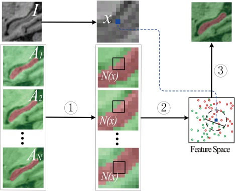
The framework of local label learning (LLL) method, consisting of steps: (1) candidate training set construction, (2) feature extraction, and (3) local SVM classification. [Color figure can be viewed in the online issue, which is available at http://wileyonlinelibrary.com.]
Candidate training set construction
To learn an image segmentation classifier for each voxel of the target image, a set of voxel‐wise training samples is identified from the registered atlases. Since the image registration of atlases cannot achieve perfect alignment of all image voxels across images, it is not appropriate to directly take the corresponding voxel of the voxel considered in each atlas as a training sample. To achieve better correspondence between voxels of the target and atlas images, a local search strategy can be used to find the best match in each atlas for the target image voxels [Wang et al., 2011b]. However, the local searching for the best match is computationally expensive if not impossible. Such a strategy also limits the number of training samples obtained no more than the number of atlases, which may require a special treatment for learning algorithms in studies with a limited number of atlases [Wang et al., 2011b].
Instead of obtaining only one sample from each atlas, we adopt a local patch based method [Coupe et al., 2011; Rousseau et al., 2011]. Given one voxel x of the target image, as illustrated in Figure 1, voxels in its neighborhood of all atlases are used as training samples. Particularly, we take a cube‐shaped neighborhood and get candidate training samples from atlases, where r is the neighborhood radius, is a feature vector extracted from voxel j of the ith atlas by the feature extraction method to be described next, and each candidate training sample's segmentation label is , same to its atlas label. When , only the corresponding voxel in each atlas is used as a training sample.
The candidate training samples from a local patch have different degrees of similarity to the target voxel to be labeled. A hybrid of SVM and kNN can identify balanced positive and negative training samples, the most similar to the target image voxel considered, and learn an effective and efficient SVM classifier based on the balanced training samples. It is worth noting that unlike the affine image registration used in [Coupe et al., 2011; Rousseau et al., 2011], we adopt a non‐rigid image registration algorithm for registering the target and atlas images so that a smaller neighborhood can be used in our algorithm, which makes the trained classifier more resistant to noise/outliers.
Feature extraction
As demonstrated in several subcortical segmentation studies [Fischl et al., 2002; Tu et al., 2008], image intensity information solely is not good enough for distinguishing different subcortical structures since most subcortical structures share similar intensity patterns in MR images. To address such a problem, in the learning based segmentation methods, more discriminative features are often extracted from MR images [Morra et al., 2010; Powell et al., 2008; Tu et al., 2008]. However, such a strategy has not been widely employed for label fusion in atlas‐based segmentation studies.
In our method, a set of features is extracted for capturing texture information of subcortical structures [Toriwaki and Yoshida, 2009]. The features extracted for each voxel include intensities in its neighborhood of size , and outputs of the first order difference filters (FODs), the second order difference filters (SODs), 3D Hyperplane filters, 3D Sobel filters, Laplacian filters, and Range difference filters [Toriwaki and Yoshida, 2009]. All of them are concatenated to form a feature vector with 367 elements.
Given an image I, FODs and SODs, capable of detecting intensity change along a line segment, can be computed as and + , respectively, where is I's intensity at voxel and θ are two rotation angles, r is the distance from to the voxels considered. In this study, , and were used for the first and second order difference filters.
Three‐dimensional Hyperplane filters and 3D Sobel filters are extensions of the first order difference filters and can be formulated as , where P is a kernel operator (for Hyperplane filters , while for 3D Sobel filters ), denotes convolution operation, and denote two planes along x axes of image I at position and . It is worth noting that the above two filters are directional. Filters along directions of y and z can be similarly implemented.
Laplacian filters are isotropic and can be treated as extensions of the second order difference filters. They can be formulated as where denotes voxels in the neighborhood of voxel excluding itself. Depending on the number of voxels used, Laplacian filter is also referred to as p‐neighbor Laplacian.In this study, three filters, namely 6−neighbor Laplacian, 18−neighbor Laplacian and 26‐neighbor Laplacian, implemented in the neighborhood were used for feature extraction.
The range difference filter computes the difference between maximal and minimal values in a given neighborhood of each voxel and can be formulated as , where denotes voxels in a given neighborhood of , and get the maximal value and the minimal value of the input, respectively. Three neighborhood sizes, including 7‐neighbor, 19‐neighbor, and 27‐neighbor, extracted in the neighborhood were used in this study for extracting features. Some filtering outputs of a randomly selected image are shown in Figure 2.
Figure 2.
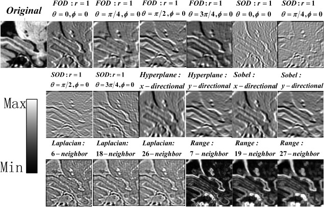
Feature extraction for a randomly selected image by applying filters with different parameters. The displayed filtering outputs are scaled to have the same intensity range as the intensity indicator.
In this study, to account for difference of intensity distributions across atlases and the target image, before feature extraction for voxel , we normalized the intensities of voxels in a cube patch centered at with a neighborhood size of . Particularly, mean value and standard deviation of intensities of all voxels in the cube patch were first computed, and then the intensity of each voxel in this cube patch was subtracted by the mean value and divided by the standard deviation.
Local SVM classification
Once the image features are extracted for both the target image voxel v and its corresponding candidate training samples, including positive samples and negative samples, a kNN strategy based SVM classification algorithm is adopted to build a classifier [Zhang et al., 2006].
In particular, approximately k nearest neighboring samples of the target image voxel are identified from the candidate training samples based on Euclidean distances between their feature vectors and the target image voxel's feature vector, including positive nearest neighboring samples and negative nearest neighboring samples, constituting a balanced training set, as illustrated by samples in the dashed black circle in Figure 1.
A SVM classifier is built on the identified training set and then used to classify the target voxel . As the features might contain redundant information, we adopt an L1‐regularized SVM method for obtaining a sparse model [Yuan et al., 2010]. The L1‐regularized SVM classifier can be obtained by solving an optimization problem:
| (7) |
where donates L1 norm.
The L1‐regularized SVM optimization problem can be solved by a coordinate descent method [Yuan et al., 2010]. In particular, our algorithm implementation used a publicly available software package LIBLINEAR (http://www.csie.ntu.edu.tw/~cjlin/liblinear/) [Fan et al., 2008]. The L1‐regularized SVM often produces a sparse solution of , and nonzero elements of are informative features selected. Once we get , the label of target image voxel can be estimated as
| (8) |
The LLL algorithm is summarized as
LLL ALGORITHM
Inputs: One target image I to be segmented, N atlases that have been spatially registered to the target image space, where is the ith atlas image and is its associated segmentation label.
Output: Label map L of the target image I.
Begin:
For each voxel x in the target image
Obtain candidate training samples and compute their image feature vectors.
Find positive training samples and negative training samples respectively from the candidate training set based on Euclidean distances between feature vectors of the testing and training samples.
Training a classifier based on the selected training samples using L1‐regularized SVM with a linear kernel.
Estimate label of the target image voxel x by applying the SVM classifier to its feature vector.
End for
End
Segmentation of Hippocampus
All MR images were registered to the MNI152 space using affine registration, and these aligned images were resampled to have a voxel size of 1 × 1 × 1 . For each of the left and right hippocampi, a bounding box was generated to cover the whole hippocampus in the MNI152 space following the procedure described in [Morra et al., 2009b]. In particular, all the atlases were scanned to find the minimum and maximum x, y, z positions of the hippocampus and the size of seven voxels was added in each direction to cover the hippocampus of unseen testing images.
Atlas Selection and Image Registration
For segmenting a target image, an atlas selection strategy was adopted to select the most similar atlases. The similarity between the target image and an atlas image was evaluated based on normalized mutual information (NMI) of image intensities within the bounding box [Aljabar et al., 2009]. In this study, we chose the top 20 most similar atlases [Morra et al., 2009b]. All the selected atlas images were independently registered to the target image using a nonlinear, cross‐correlation‐driven image registration algorithm, namely ANTs (version 1.9x) [Avants et al., 2008], with the command: ANTS 3 ‐m CC [target.nii, source.nii, 1, 2] –i 100x100x10 –o output.nii ‐t SyN[0.25] –r Gauss[3,0].
Initial Segmentation With Probabilistic Voting
To reduce the computation cost, the probabilistic voting strategy was adopted to get an initial segmentation result of the target image. For each voxel of the target image, we got the probability value of the voxel belonging to the hippocampus. The segmentation result of voxels with 100% certainty (probability value of 1 or 0) was directly taken as the final segmentation result. Then the local label learning focused on voxels with probability values greater than 0 and smaller than 1.
Parameter Tuning
The parameters of our algorithm were determined empirically based on Dataset A, including the neighborhood radius r for obtaining the candidate training samples and the parameter k for kNN. A leave‐one‐out validation was adopted to tune the parameters for achieving the optimal segmentation performance. Particularly, the searching range of r was {0, 1, 2, 3}, k was selected from {200, 300, 400, 500}. In particular, when , all available training samples were used in the SVM classifier training. We used the default value for parameter C of the L1‐regulzaried SVM as recommended in [Fan et al., 2008]. We also performed the segmentation by replacing the SVM classifier with a kNN classifier. The performance of the a kNN classifier based segmentation was evaluated with k selected from {1, 5, 10, 20, 50, 100, 150, 200, 250, 300, 400, 500}.
Feature Selection Analysis
To investigate which features are informative for the classification, we identified features most frequently selected by SVM classifiers for the segmentation of right hippocampus for images of Dataset A. As classifiers at different locations of the hippocampal structure may select different features, we focused on classifiers for voxels located at the boundary of the hippocampus. In particular, for each image of Dataset A, we first identified the boundary of its hippocampal structure, then found the features selected by the classifiers, i.e., those corresponding to non‐zero elements of , for different boundary voxels, and finally we obtained the frequency of features selected by different classifiers. The mean of frequencies of features selected for the segmentation of images of Dataset A was also obtained.
Comparison With State‐of‐the‐Art Label Fusion Methods
The proposed algorithm was compared with state of the art label fusion algorithms, including majority voting, STAPLE, LWGU [Sabuncu et al., 2010], LWINV [Wang et al., 2011b], and NLP [Coupe et al., 2011; Rousseau et al., 2011]. The parameters of LWGU, LWINV, and NLP were tuned based on Dataset A using cross‐validation. For LWGU, patch radius r and need to be determined. In particular, was adaptively set to , , and was set to 1e‐20 for numerical stability. The optimal value of r was 1, selected from {1, 2, 3}. For LWINV's parameters, including p and patch radius r, the optimal value of p was , selected from , while the optimal value of r was 1, selected from {1, 2 3}. For NLP, there are three parameters, including patch radius r, search volume V, and . The optimal value of r was 1, selected from {1, 2, 3}. The optimal value of V was , selected from { , }, was adaptively set to , and was set to 1e‐20 for numerical stability. The NLP label fusion method was performed based on atlases nonlinearly registered to the target image space, instead of those registered with affine transformation [Coupe et al., 2011; Rousseau et al., 2011].
Validation of the Segmentation Performance Across Different Datasets
We evaluated our method across different datasets. In particular, we segmented each image of Dataset A (1.5 T SIEMENS/GE scanners) with atlas images obtained from Dataset B (3.0 T SIEMENS/GE scanners) excluding that from the same subject of the image of Dataset A under consideration, and segmented each image of Dataset B with atlas images obtained from Dataset A excluding that from the same subject of the image of Dataset B under consideration. It is worth noting that images of Dataset A and Dataset B were acquired with different scanners and from subjects of different diagnostic groups, including AD, MCI, and NC. We also segmented each image of Dataset C (3.0 T SIEMENS scanner) with atlas images obtained from Dataset A (1.5 T SIEMENS/GE scanners) or Dataset B (3.0 T SIEMENS/GE scanners).
Validation of the Segmentation Performance Based on Public Available Data
Besides MR images from studies of Alzheimer's disease, we also validated our method based on a publicly available dataset of nonepileptic subjects and epilepsy patients [Jafari‐Khouzani et al., 2011]. Using the training data of 25 subjects as atlases, we obtained segmentation results of the testing data using our method, LWGU, LWINV, and NLP with the same parameters used in the previous experiments. As these images have anisotropic spatial resolution, we first interpolated the voxel size to 1 × 1 × 1 mm3 before segmentation. Then, after the segmentation, we interpolated the image back to its original resolution for evaluating the segmentation performance. The performance of these methods was evaluated by the dataset provider based on 11 metrics and compared with two algorithms: Brain Parser [Tu et al., 2008] and a multi‐atlas based segmentation method [Aljabar et al., 2007].
Evaluation Metrics
The segmentation performance of each method was evaluated using leave‐one‐out cross‐validation. We adopted the metrics used in [Jafari‐Khouzani et al., 2011] except “Specificity” due to the reason that it varies with the size of background. Given manual segmentation label E and the automated segmentation result F, these metrics can be calculated as:
,
,
,
,
,
,
Hausdorff Distance: , where ,
Hausdorff 95 Distance (HD95) is similar to Hausdorff Distance, except that 5% data points with the largest distance are removed before the calculation,
Average Symmetric Surface Distance: ,
Root Mean Square Distance: .
In above metrics, BE denotes boundary voxels of the segmentation denotes boundary voxels of the segmentation F, is the Euclidian distance between two points, is the cardinality of a set, and is the volume of segmentation X.
The first four metrics have been widely used in image segmentation studies and they are related to each other. The relative volume difference metric can reveal the segmentation method's capability for detecting volume changes, although it does not directly measure the overlap between segmentation labels. The last five metrics, measuring surface distance between segmentation results, characterize the boundary difference.
Hippocampal Volumetry for Alzheimer's Disease
A volumetric analysis was carried out to test the capacity of each method for capturing the volume difference among NC, MCI, and AD, based on the available 3.0 T images in Dataset B and Dataset C. Based on the segmentation results, each subject's hippocampal volumes were computed and normalized by its total intracranial volume (TIV) estimated by VBM8 (http://dbm.neuro.uni-jena.de/vbm/download/). In particular, each subject's hippocampal volume was divided by its TIV and then multiplied by mean of TIVs of all subjects of Dataset B and Dataset C. We also performed two sample t tests, computed standardized effect sizes (Cohen's d), and estimated sample size of each group for different methods to detect a difference in total hippocampal volumes (left + right) between NC group and MCI group, as well as between NC group and AD group. For the sample size estimation, Type I error rate was set to 0.05, and power was set to 0.8 [Eng, 2003].
RESULTS
Initial Segmentation With Probabilistic Voting
The experiment results revealed that voxels labeled by the probabilistic voting [Eq. (3)] as either hippocampus (+1) or background (−1) with 100% certainty were correctly segmented with a correct rate close to 100%. On average, only one voxel labeled with 100% certainty was misclassified in each image in Datasets A, B, and C. Figure 3 shows the initial segmentation result on one randomly selected test image. Therefore, our algorithm can focus on voxels labeled by the probabilistic voting with probability values greater than 0 and smaller than 1. In particular, about 98% of the background and 20% of the foreground voxels were labeled with 100% certainty for subjects of Dataset A within the bounding box of 44 × 63 × 64 of one side of the hippocampus.
Figure 3.
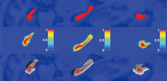
The initial segmentation result of a randomly selected test image based on the probabilistic voting. The first row shows three slices of the test image with manual segmentation label. The probabilistic voting results are shown in the second row and the color bar indicates the probability of a voxel belonging to the hippocampus. The voxels belonging to the hippocampus or not with 100% certainty (probability value is 1: red or 0: blue) are overlaid on the test image in the third row. First column: horizontal; second column: sagittal; third column: coronal. [Color figure can be viewed in the online issue, which is available at http://wileyonlinelibrary.com.]
Parameter Tuning
Figure 4 shows average Dice index values of segmentation results of the right hippocampus with r varying from 0 to 3. For the SVM based segmentation, the segmentation performance improved first as the number of training samples K increased and reached its maximal when K was 400, then the performance degraded if K was greater than 400. The optimal value of r was 1 and the optimal value for K was 400. The segmentation performance improvement with the increase of the number of training samples (<400) might be due to the relieved curse of dimensionality. However, the segmentation performance degraded if too many samples, e.g., 500 samples, were used in the SVM training, indicating that noisy training samples (located far away from the voxel considered) might be involved in the classifier training. The segmentation performance when was worse than when , possibly due to that the limited training samples might not able to provide sufficiently discriminative information for building robust classifiers. The segmentation performance degraded as r varying from 1 to 3, indicating that irrelevant samples may have been used in the classifier training when larger searching radius r was used.
Figure 4.
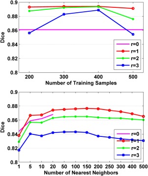
The average Dice index values of segmentation results of the right hippocampus for dataset A with different numbers of training samples and r varying from 0 to 3. Top: SVM classifier based segmentation results. Bottom: kNN classifier based segmentation results. For the SVM classifier based segmentation, all available training samples (20 in total) were used without selection when r = 0. For the kNN classifier based segmentation, all available training samples were used. [Color figure can be viewed in the online issue, which is available at http://wileyonlinelibrary.com.]
Similar to the SVM classifier based segmentation, the kNN classifier based segmentation performance improved and then degraded with the increase of k, the number of nearest neighbors used in the classification. The segmentation performance degraded as r varying from 1 to 3. However, the segmentation performance when was better than when . The best Dice index was 0.877, achieved with 150 nearest neighbors and . Overall, the segmenation performance of kNN classifiers was worse than that of SVM classifiers, suggesting that the sophisticated SVM classifiers should be used in the segmentation.
Feature Selection Analysis
The frequency of features used in the segmentation is shown in Figure 5. On average, about 7% features were selected for the segmentation. These results indicated that both intensity information and filtering outputs played important roles in the segmentation. The top ten most frequently selected features are summarized in Table 2.
Figure 5.
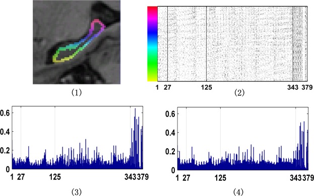
Frequency of features used in the segmentation. (1) One randomly selected image with the hippocampus boundary voxels shown in different colors. (2) Features selected in the segmentation. Each row indexed by the color bar shown at the left corresponds to the boundary voxel in the same color shown in (1). The x‐axis is the feature index (1–27: intensity features in the neighborhood of , 1–125: intensity features in the neighborhood of , 1:343: intensity features in the neighborhood of , 344–367: filtering outputs). (3) Frequency of features selected for the segmentation of the image shown in (1). (4) Mean of frequencies of features selected for the segmentation of images of dataset A. [Color figure can be viewed in the online issue, which is available at http://wileyonlinelibrary.com.]
Table 2.
Top 10 most frequently selected features on average for the segmentation of dataset A
| Rank | Feature type | Parameter | |
|---|---|---|---|
| 1 | Laplacian filter | 6‐Neighbor | |
| 2 | Laplacian filter | 26‐Neighbor | |
| 3 | Intensity | [0, 0, 0] | |
| 4 | Intensity | [−1, 0, 0] | |
| 5 | Laplacian filter | 18‐neighbor | |
| 6 | Intensity | [0, −1, 1] | |
| 7 | Intensity | [0, 1, 0] | |
| 8 | FOD |
|
|
| 9 | Intensity | [0, 1, −1] | |
| 10 | Intensity | [0, 0, 1] |
Comparison With State‐of‐the‐Art Label Fusion Methods
Figures 6 to 8 show box plots of segmentation performance measures of majority voting, STAPLE, LWGU, LWINV, NLP, as well as LLL, based on Datasets A, B, and C, respectively. The mean values of the segmentation performance measures and P values of single‐sided paired t tests for comparing LLL with others are reported in Tables 3, 4 to 5. All the results demonstrated that the proposed method performed consistently better than other label fusion methods.
Figure 6.
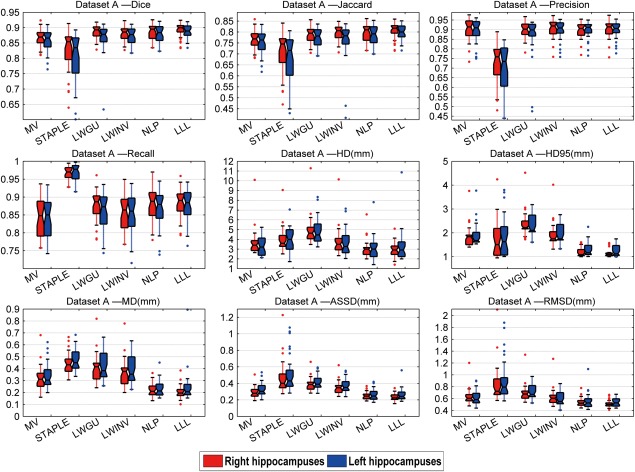
Box plots of the results for the dataset A. On each box, the central mark is the median, and edges of the box are the 25th and 75th percentiles. Whiskers extend from each end of the box to the adjacent values in the dataset and the extreme values within 1 interquartile range from the ends of the box. Outliers are data with values beyond the ends of the whiskers. [Color figure can be viewed in the online issue, which is available at http://wileyonlinelibrary.com.]
Figure 8.
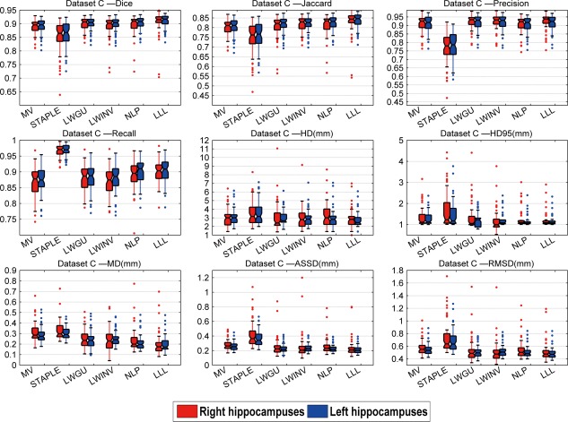
Box plots of the results for the dataset C. On each box, the central mark is the median, and edges of the box are the 25th and 75th percentiles. Whiskers extend from each end of the box to the adjacent values in the dataset and the extreme values within 1 interquartile range from the ends of the box. Outliers are data with values beyond the ends of the whiskers. [Color figure can be viewed in the online issue, which is available at http://wileyonlinelibrary.com.]
Table 3.
Results of dataset A: Means of the metrics and P values of paired‐tests comparing different methods with LLL method for both left and right hippocampus
| MV P value (L/R) | STAPLE P value (L/R) | LWGU P value (L/R) | LWINV P value (L/R) | NLP P value (L/R) | LLL | |
|---|---|---|---|---|---|---|
| Dice (L/R) | 0.860/0.868; 3.4e‐6/5.2e‐10 | 0.802/0.824; 5.2e‐7/1.1e‐6 | 0.872/0.881; 1.7e‐5/4.5e‐6 | 0.860/0.886; 1.9e‐2/1.3e‐3 | 0.882/0.888; 3.3e‐2/4.8e‐2 | 0.886/0.894 |
| Jaccard (L/R) | 0.755/0.767; 1.6e‐6/5.8e‐10 | 0.677/0.707; 1.1e‐7/3.0e‐7 | 0.775/0.789; 1.4e‐5/4.7e‐6 | 0.760/0.796; 1.3e‐2/1.1e‐3 | 0.789/0.799; 3.7e‐2/4.8e‐2 | 0.796/0.814 |
| Precision (L/R) | 0.894/0.900; 2.7e‐1/2.3e‐1 | 0.694/0.724; 1.2e‐12/2.6e‐12 | 0.864/0.898; 4.2e‐2/2.9e‐2 | 0.897/0.908; 3.5e‐1/9.7e‐1 | 0.898/0.899; 3.2e‐1/3.9e‐2 | 0.899/0.904 |
| Recall (L/R) | 0.834/0.843; 1.3e‐7/3.9e‐8 | 0.971/0.970; 1.0/1.0 | 0.863/0.876; 2.1e‐4/3.5e‐3 | 0.853/0.860; 1.0e‐7/1.8e‐7 | 0.870/0.880; 8.5e‐3/9.7e‐2 | 0.877/0.884 |
| HD (mm) (L/R) | 3.930/3.750; 7.8e‐1/1.6e‐4 | 4.100/3.990; 4.0e‐1/1.2e‐6 | 4.890/4.870; 5.5e‐2/1.3e‐9 | 3.700/3.730; 6.4e‐1/7.0e‐4 | 3.400/3.145; 9.2e‐1/3.9e‐2 | 3.917/2.909 |
| HD95 (mm) (L/R) | 1.820/1.780; 3.1e‐9/6.3e‐11 | 1.930/1.710; 3.7e‐4/9.2e‐4 | 2.220/2.300; 2.4e‐15/7.2e‐16 | 1.890/1.800; 1.5e‐11/2.5e‐10 | 1.187/1.097; 4.2e‐2/2.0e‐1 | 1.121/1.083 |
| MD (mm) (L/R) | 0.340/0.320; 2.4e‐3/2.9e‐6 | 0.470/0.440; 4.8e‐11/1.0e‐16 | 0.420/0.410; 2.7e‐6/5.1e‐10 | 0.390/0.370; 3.7e‐5/3.9e‐8 | 0.271/0.219; 7.2e‐3/2.4e‐2 | 0.244/0.203 |
| ASSD (mm) (L/R) | 0.330/0.290; 5.4e‐5/1.4e‐6 | 0.520/0.470; 2.6e‐7/2.4e‐7 | 0.410/0.390; 7.7e‐11/4.8e‐15 | 0.370/0.350; 5.8e‐8/8.7e‐12 | 0.300/0.250; 6.3e‐3/2.4e‐2 | 0.265/0.238 |
| RMSD (mm) (L/R) | 0.620/0.630; 4.7e‐1/1.4e‐6 | 0.910/0.840; 1.8e‐3/1.1e‐6 | 0.710/0.690; 1.0e‐1/4.8e‐9 | 0.661/0.620; 6.2e‐3/2.7e‐5 | 0.650/0.538; 8.3e‐3/8.0e‐3 | 0.614/0.516 |
Bold: value of LLL method is significantly (P < 0.05) better than all other methods.
Table 4.
Results of dataset B: Means of the metrics and P values of paired‐tests comparing the different methods with LLL method for both side of the hippocampus
| MV P value (L/R) | STAPLE P value (L/R) | LWGU P value (L/R) | LWINV P value (L/R) | NLP P value (L/R) | LLL | |
|---|---|---|---|---|---|---|
| Dice (L/R) | 0.872/0.876; 9.1e‐11/4.2e‐13 | 0.830/0.836; 5.6e‐7/9.0e‐8 | 0.887/0.892; 5.5e‐9/5.2e‐10 | 0.891/0.896; 1.1e‐7/1.5e‐8 | 0.898/0.902; 8.6e‐6/5.1e‐5 | 0.907/0.910 |
| Jaccard (L/R) | 0.774/0.780; 2.6e‐11/3.2e‐13 | 0.716/0.724; 1.3e‐7/1.9e‐8 | 0.797/0.805; 2.6e‐9/5.0e‐10 | 0.808/0.819; 2.2e‐5/2.8e‐3 | 0.816/0.822; 8.5e‐6/5.2e‐5 | 0.831/0.835 |
| Precision (L/R) | 0.898/0.898; 9.5e‐4/2.0e‐3 | 0.737/0.743; 1.1e‐11/1.1e‐12 | 0.912/0.901; 5.7e‐3/4.1e‐7 | 0.915/0.915; 2.3e‐1/5.5e‐1 | 0.911/0.908; 1.9e‐3/6.5e‐4 | 0.918/0.915 |
| Recall (L/R) | 0.854/0.861; 2.5e‐7/4.4e‐9 | 0.967/0.969; 1.0/1.0 | 0.892/0.889; 1.9e‐5/6.3e‐9 | 0.865/0.873; 8.4e‐9/2.1e‐10 | 0.890/0.899; 5.1e‐6/2.5e‐4 | 0.900/0.907 |
| HD (mm) (L/R) | 3.257/3.347; 3.6e‐2/1.8e‐2 | 4.111/3.711; 4.9e‐5/2.9e‐4 | 3.900/3.631; 1.3e‐7/1.6e‐3 | 3.202/3.130; 4.5e‐2/1.7e‐1 | 3.004/3.062; 3.7e‐1/1.2e‐1 | 2.954/2.907 |
| HD95 (mm) (L/R) | 1.300/1.389; 3.7e‐3/3.7e‐5 | 1.928/1.763; 2.1e‐4/3.4e‐4 | 1.618/1.573; 3.4e‐8/3.2e‐7 | 1.320/1.360; 1.1e‐3/4.2e‐4 | 1.132/1.069; 3.0e‐2/2.9e‐1 | 1.055/1.055 |
| MD (mm) (L/R) | 0.336/0.333; 3.2e‐8/2.6e‐8 | 0.342/0.345; 2.7e‐13/1.2e‐12 | 0.457/0.438; 3.2e‐12/4.7e‐12 | 0.370/0.340; 9.8e‐9/8.2e‐8 | 0.198/0.193; 8.6e‐5/1.6e‐4 | 0.175/0.174 |
| ASSD (mm) (L/R) | 0.291/0.287; 6.6e‐10/4.0e‐11 | 0.457/0.435; 4.2e‐7/1.9e‐7 | 0.358/0.343; 9.6e‐14/6.7e‐14 | 0.330/0.320; 1.2e‐11/4.7e‐12 | 0.226/0.217; 9.5e‐5/9.2e‐5 | 0.204/0.199 |
| RMSD (mm) (L/R) | 0.593/0.600; 7.3e‐9/2.1e‐7 | 0.821/0.778; 3.4e‐6/3.5e‐6 | 0.688/0.669; 1.0e‐12/6.7e‐10 | 0.570/0.600; 1.1e‐5/2.3e‐6 | 0.509/0.499; 1.4e‐4/6.1e‐4 | 0.479/0.474 |
Bold: value of LLL method is significantly (P < 0.05) better than all other methods.
Table 5.
Results of dataset C: Means of the metrics and P values of paired‐tests comparing the different methods with LLL method for both side of the hippocampus
| MV P value (L/R) | STAPLE P value (L/R) | LWGU P value (L/R) | LWINV P value (L/R) | NLP P value (L/R) | LLL | |
|---|---|---|---|---|---|---|
| Dice (L/R) | 0.891/0.888; 1.5e‐14/3.0e‐4 | 0.860/0.853; 9.2e‐16/2.2e‐8 | 0.897/0.891; 3.7e‐10/2.1e‐10 | 0.899/0.900; 4.3e‐10/1.3e‐2 | 0.902/0.895; 3.2e‐6/1.4e‐5 | 0.909/0.906 |
| Jaccard (L/R) | 0.804/0.800; 5.9e‐15/2.8e‐5 | 0.757/0.748; 1.4e‐16/1.9e‐9 | 0.814/0.804; 1.7e‐10/2.6e‐11 | 0.817/0.819; 2.0e‐10/6.7e‐3 | 0.821/0.811; 2.5e‐6/2.9e‐6 | 0.834/0.831 |
| Precision (L/R) | 0.910/0.910; 1.0e‐4/6.3e‐5 | 0.778/0.770; 5.4e‐30/5.0e‐22 | 0.917/0.924; 9.3e‐1/4.5e‐1 | 0.917/0.923; 9.1e‐1/2.1e‐1 | 0.906/0.907; 2.1e‐9/4.5e‐10 | 0.915/0.924 |
| Recall (L/R) | 0.875/0.870; 6.3e‐14/2.2e‐3 | 0.968/0.966; 1.0/1.0 | 0.884/0.880; 2.3e‐15/5.9e‐2 | 0.881/0.865; 2.1e‐14/3.5e‐13 | 0.900/0.886; 8.7e‐3/1.6e‐2 | 0.905/0.892 |
| HD (mm) (L/R) | 3.035/2.986; 1.4e‐4/1.9e‐1 | 3.551/3.635; 3.5e‐6/3.1e‐6 | 2.950/3.040; 5.5e‐2/9.6e‐2 | 2.960/3.070; 2.2e‐3/2.0e‐1 | 3.000/3.174; 1.2e‐2/5.9e‐3 | 2.770/2.893 |
| HD95 (mm) (L/R) | 1.159/1.231; 6.6e‐3/5.0e‐2 | 1.430/1.579; 4.2e‐7/3.0e‐5 | 1.147/1.210; 8.1e‐2/3.6e‐2 | 1.135/1.170; 2.7e‐2/3.7e‐1 | 1.084/1.183; 3.8e‐1/1.5e‐2 | 1.081/1.124 |
| MD (mm) (L/R) | 0.287/0.310; 5.1e‐9/1.1e‐8 | 0.302/0.333; 4.6e‐19/7.7e‐12 | 0.240/0.270; 2.3e‐3/6.8e‐6 | 0.254/0.270; 1.7e‐5/3.2e‐3 | 0.213/0.235; 1.3e‐6/3.8e‐7 | 0.195/0.201 |
| ASSD (mm) (L/R) | 0.259/0.280; 8.1e‐15/7.9e‐4 | 0.370/0.416; 1.2e‐17/7.5e‐10 | 0.228/0.250; 6.9e‐3/1.2e‐3 | 0.235/0.250; 5.9e‐9/4.9e‐2 | 0.228/0.258; 1.3e‐5/3.0e‐5 | 0.212/0.233 |
| RMSD (mm) (L/R) | 0.547/0.574; 6.6e‐14/5.9e‐4 | 0.676/0.735; 6.6e‐15/6.1e‐9 | 0.507/0.526; 4.6e‐2/7.9e‐2 | 0.520/0.536; 3.1e‐9/1.9e‐2 | 0.509/0.546; 1.2e‐5/1.5e‐5 | 0.489/0.511 |
Bold: value of LLL method is significantly (P < 0.05) better than all other methods.
Figure 7.
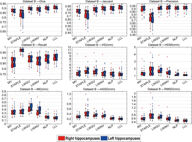
Box plots of the results for the dataset B. On each box, the central mark is the median, and edges of the box are the 25th and 75th percentiles. Whiskers extend from each end of the box to the adjacent values in the dataset and the extreme values within 1 interquartile range from the ends of the box. Outliers are data with values beyond the ends of the whiskers. [Color figure can be viewed in the online issue, which is available at http://wileyonlinelibrary.com.]
Hippocampal volume differences between results of the manual segmentation and automatic segmentation are shown in Figure 9 and Table 6. Pearson correlation coefficients between hippocampal volumes estimated by the manual segmentation and by different methods are also reported in Table 6. These results demonstrated that our proposed method could better estimate the hippocampal volume, although small volume differences do not necessarily mean accurate segmentation results. For visual inspection, Figure 10 shows segmentation results of subjects randomly selected from each dataset.
Figure 9.
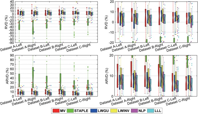
Relative volume differences (RVD) (first row) and absolute value of RVD (ARVD) (second row) between the segmentation results of automatic methods and the manual label on the three datasets. Figures at the right side are the zoomed in version of figures at the left side. On each box, the central mark is the median, and edges of the box are the 25th and 75th percentiles. Whiskers extend from each end of the box to the adjacent values in the dataset and the extreme values within 1 times the interquartile range from the ends of the box. Outliers are data with values beyond the ends of the whiskers. [Color figure can be viewed in the online issue, which is available at http://wileyonlinelibrary.com.]
Table 6.
Relative volume difference (RVD), absolute value of RVD (ARVD), and correlation between manual segmentation and segmentation results obtained by automatic methods
| Methods | MV; RVD (%); ARVD (%) | STAPLE RVD (%); ARVD (%) | LWGU; RVD (%); ARVD (%) | LWINV; RVD (%); ARVD (%) | NLP; RVD (%); ARVD (%) | LLL; RVD (%); ARVD (%) |
|---|---|---|---|---|---|---|
| Dataset A left correlation | 5.7 ± 11.5; 10.7 ± 6.8; 0.922 | −37.3 ± 24.7; 37.3 ± 24.7; 0.764 | 2.2 ± 7.8; 6.7 ± 4.5; 0.956 | 4.8 ± 9.8; 9.2 ± 5.5; 0.942 | 1.9 ± 8.7; 7.5 ± 4.6; 0.952 | 1.9 ± 8.6; 7.1 ± 5.1; 0.952 |
| Dataset A right correlation | 6.0 ± 12.6; 11.3 ± 7.9; 0.897 | −45.1 ± 31.1; 45.1 ± 31.1; 0.716 | −2.2 ± 19.5; 11.7 ± 15.6; 0.795 | 4.3 ± 10.8; 9.3 ± 6.7; 0.924 | 2.8 ± 9.7; 8.2 ± 5.8; 0.931 | 2.1 ± 9.1; 7.5 ± 5.5; 0.940 |
| Dataset B left correlation | 3.3 ± 12.2; 10.5 ± 6.8; 0.918 | −33.5 ± 22.2; 33.5 ± 22.2; 0.826 | 4.0 ± 8.9; 8.1 ± 5.3; 0.952 | 4.2 ± 9.8; 8.9 ± 5.7; 0.945 | 0.7 ± 8.7; 6.7 ± 5.4; 0.957 | 0.6 ± 8.3; 6.3 ± 5.3; 0.959 |
| Dataset B Right correlation | 4.1 ± 13.8; 11.5 ± 8.5; 0.889 | −35.6 ± 27.9; 35.6 ± 27.9; 0.759 | 5.2 ± 9.9; 9.4 ± 5.8; 0.937 | 5.0 ± 11.1; 10.0 ± 6.8; 0.926 | 2.0 ± 9.4; 7.7 ± 5.5; 0.943 | 1.6 ± 9.1; 7.4 ± 5.3; 0.944 |
| Dataset C left correlation | 4.0 ± 8.7; 7.4 ± 6.0; 0.923 | −27.8 ± 19.9; 27.8 ± 19.9; 0.803 | 4.4 ± 7.5; 7.0 ± 5.0; 0.945 | 6.0 ± 8.7; 8.2 ± 6.6; 0.914 | 2.1 ± 8.4; 6.1 ± 6.1; 0.923 | 3.3 ± 8.6; 6.0 ± 6.1; 0.947 |
| Dataset C right correlation | 3.5 ± 8.9; 7.8 ± 5.5; 0.932 | −25.9 ± 15.3; 25.9 ± 15.3; 0.902 | 3.3 ± 8.3; 7.3 ± 5.1; 0.939 | 3.6 ± 8.5; 7.5 ± 5.3; 0.937 | 0.3 ± 8.4; 6.5 ± 5.2; 0.940 | 0.8 ± 8.1; 6.3 ± 5.0; 0.945 |
Highest Pearson correlation coefficients are shown in bold.
Figure 10.
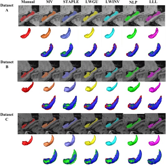
Hippocampal segmentation results obtained by different methods. One subject was randomly chosen from each dataset. For each subject, the first row shows the segmentation results produced by different methods, the second row demonstrates their corresponding surface rendering results, and the difference between results of manual and automatic segmentation methods was showed in the third row (red: manual segmentation results, green: automated segmentation results, blue: overlap between manual and automated segmentation results). [Color figure can be viewed in the online issue, which is available at http://wileyonlinelibrary.com.]
The performance of STAPLE was relatively poor, as similarly reported in other atlas‐based segmentation studies [Artaechevarria et al., 2009; Khan et al., 2011; Langerak et al., 2010]. In our experiment, STAPLE had the worst performance evaluated by most of the performance metrics, except recall index and mean distance. The visual inspection and volume difference information revealed that STAPLE was prone to generating segmentation results larger than the manual segmentation results.
The overall performance of majority voting was better than STAPLE. Particularly, majority voting had a higher precision index and a lower recall index, indicating the hippocampal segmentation volume of this method was smaller than that of the manual segmentation compared with other methods, consistent with the results (negative RVD) reported in Table 6.
LWGU and LWINV had similar performance, better than both STAPLE and majority voting. This finding was consistent with results reported in [Artaechevarria et al., 2009; Sabuncu et al., 2010], and further justified the effectiveness of spatially adaptive image similarity measures for characterizing the image registration accuracy in multi‐atlas based image segmentation. NLP performed better than LWGU and LWINV, providing supportive evidence that better fusion performance can be obtained by relaxing the one‐to‐one correspondence constrains.
For all the datasets, the proposed method achieved the best overall performance. In particular, our method had the best value on most metrics, including Dice, Jaccard, MD, ASSD, and RMSD, confirmed by paired single‐sided t test as summarized in Tables 3, 4, 5. The Recall index of our method was just lower than STAPLE's, indicating that our method was able to generate segmentation results that better covered the foreground region of the manual segmentation. For most of the metrics, our method had fewer outliers compared with other methods, indicating that our method might be more robust than other methods. Our method produced segmentation volumes with the least difference from the manual segmentation results for most datasets, except for the left hippocampus of Dataset A, as indicated by the results shown in Figure 9 and Table 6. It is worth noting that we presented measures of both RVD and absolute value of RVD. RVD itself contains directional information of the volume difference, and its absolute value reflects the absolute difference.
Validation of the Segmentation Performance Across Different Datasets
As shown in Table 7, for images obtained from ADNI, i.e., Dataset A and Dataset B, acquired with scanners of different makers and different field strengths, our method have achieved robust segmentation performance. However, the segmentation performance of our method for images of Dataset C with atlases obtained from Dataset A or Dataset B was worse than that obtained with atlases obtained from Dataset C. Such a performance difference might be caused by different imaging protocols used for image acquisition and different ethnic groups of the subjects. The images of ADNI were acquired with a standard protocol at different imaging sites and geometric distortion of images were corrected. However, the images of Dataset C were acquired without correction of geometric distortion. The difference between with and without geometric distortion correction and the difference of ethnic groups might make the image registration difficult.
Table 7.
Segmentation performance of across different datasets
| Dice index values (L/R) | |
|---|---|
| B→A(A→A) | A → B(B → B) |
| 0.887/0.893(0.886/0.894) | 0.901/0.904(0.907/0.910) |
| A→C(C→C) | B→C(C→C) |
| 0.879/0.874(0.909/0.906) | 0.883/0.875(0.909/0.906) |
X→Y: images of dataset X were used as atlases to segment images of dataset Y.
Validation on Public Available Data of Epilepsy Patients and Normal Subjects
Table 8 shows performance of the segmentation methods evaluated based on the publicly available dataset of epilepsy patients and normal subjects. Based on the published results [Jafari‐Khouzani et al., 2011], our method performed much better than the supervised learning method [Tu et al., 2008] and the multi‐atlas‐based segmentation method [Aljabar et al., 2007]. Results of statistical tests demonstrated that our method was statistically better than three other methods (LWGU, LWINV, NLP) for 6 of 10 metrics. The degree of performance improvement achieved by our method over LWGU and LWINV was similar to those reported in [Artaechevarria et al., 2009; Khan et al., 2011]. However, the improvement was statistically significant as indicated by P values of paired‐tests for comparing LLL with LWGU, LWINV, and NLP. These results also indicated that the segmentation methods performed better for images with isotropic voxels than those with highly anisotropic voxels, such as those in this public dataset (20 1.5 T images with voxel size 0.78 × 0.78 × 2.00 mm3, five 3.0 T images with voxel size 0.39 × 0.39 × 2.00 mm3).
Table 8.
Segmentation performance on the publicly available dataset of epilepsy patients and normal subjects
| Methods | Tu et al. [2008] | Aljabar et al. [2007] | LWGU; P value | LWINV; P value | NLP; P value | LLL |
|---|---|---|---|---|---|---|
| Dice | 0.64 ± 0.06 | 0.75 ± 0.07 | 0.828 ± 0.031; 7.8e‐4 | 0.828 ± 0.031; 4.4e‐4 | 0.827 ± 0.030; 1.8e‐7 | 0.831 ± 0.030 |
| Jaccard | 0.47 ± 0.06 | 0.60 ± 0.07 | 0.709 ± 0.043; 6.3e‐4 | 0.709 ± 0.043; 3.4e‐4 | 0.707 ± 0.042; 1.7e‐7 | 0.714 ± 0.042 |
| Precision | 0.50 ± 0.08 | 0.77 ± 0.07 | 0.797 ± 0.053; 2.0e‐4 | 0.797 ± 0.053; 1.6e‐4 | 0.795 ± 0.053; 4.5e‐7 | 0.802 ± 0.053 |
| Recall | 0.92 ± 0.06 | 0.74 ± 0.10 | 0.868 ± 0.039; 3.9e‐1 | 0.867 ± 0.039; 2.9e‐1 | 0.866 ± 0.039; 3.2e‐2 | 0.868 ± 0.039 |
| HD (mm) | 8.77 ± 4.30 | 4.45 ± 1.54 | 5.848 ± 5.590; 1.2e‐1 | 5.844 ± 5.591; 1.4e‐1 | 5.956 ± 5.542; 7.9e‐3 | 5.800 ± 5.606; |
| HD95 (mm) | 4.58 ± 1.68 | 2.41 ± 0.98 | 1.851 ± 0.472; 9.5e‐2 | 1.851 ± 0.468; 6.3e‐2 | 1.840 ± 0.450; 3.5e‐1 | 1.833 ± 0.473; |
| MD (mm) | 1.58 ± 0.50 | 0.50 ± 0.18 | 0.351 ± 0.128; 7.8e‐2 | 0.351 ± 0.129; 5.9e‐2 | 0.342 ± 0.125; 9.8e‐1 | 0.347 ± 0.126 |
| ASSD (mm) | 1.33 ± 0.33 | 0.55 ± 0.27 | 0.339 ± 0.095; 1.1e‐3 | 0.340 ± 0.096; 7.2e‐4 | 0.340 ± 0.094; 6.7e‐5 | 0.333 ± 0.093; |
| RMSD (mm) | 1.88 ± 0.54 | 0.95 ± 0.39 | 0.691 ± 0.165; 5.3e‐3 | 0.691 ± 0.164; 3.9e‐3 | 0.690 ± 0.160; 1.6e‐3 | 0.681 ± 0.161; |
| RVD (%) | 94 ± 37 | −4 ± 15 | 9.7 ± 11.1; 8.1e‐4 | 9.7 ± 11.1; 1.4e‐3 | 9.8 ± 11.1; 3.5e‐4 | 9.0 ± 11.0; |
| ARVD (%) | / | / | 10.6 ± 10.2; 8.8e‐3 | 10.6 ± 10.2; 1.2e‐2 | 10.7 ± 10.2; 6.7e‐3 | 10.1 ± 10.0 |
Means values with their standard deviations of the metrics are shown. Bold: value of LLL method is significantly (P < 0.05) better than all other methods.
Hippocampal Volumetry
The distributions of hippocampal volumes estimated from the segmentation results of all 3.0 T images are shown in Figure 11, and group means and standard variances of NC, MCI, and AD are summarized in Table 9. These results demonstrated that the mean volumes of segmentation results produced by our method were the closest to those obtained by manual segmentation for NC group. The segmentation results produced by the automatic methods had smaller variance than those produced by the manual segmentation as indicated by the standard deviations of volumes estimated, suggesting that automatic methods could achieve segmentation results with better consistency. The t test results confirmed the finding that the hippocampal volume is a promising biomarker for Alzheimer's disease [Morra et al., 2009a; Schuff et al., 2009; Wolz et al., 2010b]. Our method could even detect a statistically significant difference between NC and MCI with a P value smaller than the manual segmentation's. Such findings were also confirmed by the effect sizes that characterize the standard mean volume difference between NC and its counterparts. As shown in Table 9, our method had the largest effect size and the smallest sample size of all automatic methods.
Figure 11.
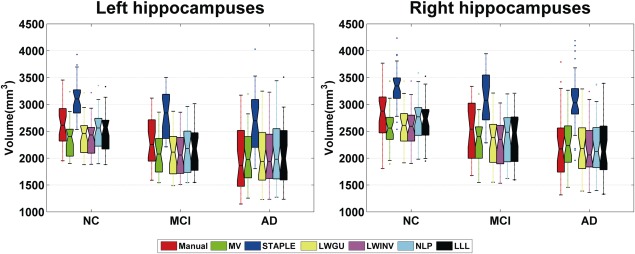
Hippocampal volumes of subjects from three diagnostic groups. On each box, the central mark is the median, and edges of the box are the 25th and 75th percentiles. Whiskers extend from each end of the box to the adjacent values in the dataset and the extreme values within 1 interquartile range from the ends of the box. Outliers are data with values beyond the ends of the whiskers. [Color figure can be viewed in the online issue, which is available at http://wileyonlinelibrary.com.]
Table 9.
Normalized hippocampal volume information of three diagnostic groups estimated by different methods, and two sample t‐tests, effect sizes, and sample sizes for different methods to detect a difference in total hippocampal volumes between NC group and MCI group, as well as between NC group and AD group
| Methods | NC | MCI | AD | ||||||
|---|---|---|---|---|---|---|---|---|---|
| Volume (mm3); left; right | Volume (mm3); left; right | t‐Test between MCI and NC (P value) | Effect size (d) | Sample size | Volume (mm3); left; right | t‐Test between AD and NC (P value) | Effect size (d) | Sample size | |
| Manual segmentation | 2,623 ± 393; 2,826 ± 450 | 2,266 ± 484; 2,482 ± 525 | 5.3e‐3 | 0.79 | 25 | 2,044 ± 586; 2,328 ± 618 | 9.0e‐5 | 1.07 | 14 |
| MV | 2,371 ± 315; 2,574 ± 366 | 2,088 ± 343; 2,317 ± 379 | 5.0e‐3 | 0.79 | 25 | 2,078 ± 474; 2,322 ± 432 | 8.2e‐3 | 0.70 | 32 |
| STAPLE | 3,114 ± 343; 3,338 ± 416 | 2,803 ± 373; 3,087 ± 399 | 6.2e‐3 | 0.77 | 26 | 2,765 ± 531; 3,177 ± 447 | 1.8e‐2 | 0.62 | 41 |
| LWGU | 2,417 ± 340; 2,610 ± 384 | 2,089 ± 386; 2,322 ± 435 | 3.8e‐3 | 0.82 | 23 | 2,055 ± 515; 2,290 ± 492 | 2.8e‐3 | 0.79 | 25 |
| LWINV | 2,397 ± 332; 2,593 ± 379 | 2,084 ± 378; 2,297 ± 427 | 3.6e‐3 | 0.82 | 23 | 2,057 ± 500; 2,235 ± 451 | 1.3e‐3 | 0.86 | 21 |
| NLP | 2,506 ± 364; 2,704 ± 403 | 2,173 ± 407; 2,394 ± 473 | 4.6e‐3 | 0.80 | 24 | 2,103 ± 566; 2,285 ± 503 | 6.7e‐4 | 0.91 | 19 |
| LLL | 2,523 ± 369; 2,736 ± 429 | 2,161 ± 418; 2,399 ± 473 | 2.8e‐3 | 0.85 | 22 | 2,108 ± 552; 2,304 ± 499 | 5.3e‐4 | 0.93 | 18 |
Effect of the Number of Atlases in Segmentation
In all above experiments, 20 atlases were used for segmenting the target image. To investigate how the number of atlases affects the segmentation performance, the segmentation performance associated with different numbers of atlases was evaluated for right hippocampus based on Dataset A. As shown in Figure 12, all the segmentation methods under study shared a similar pattern, i.e., their performance measured by a leave‐one‐out validation gradually improved with the increase of the number of atlases used in segmentation. For all the methods, an atlas selection strategy based on NMI similarity metric was used to select atlases [Aljabar et al., 2009; Collins and Pruessner, 2010; Leung et al., 2011; Wolz et al., 2010a; Wu et al., 2007]. Since LWGU and LWINV had similar performance, only LWGU was performed in this experiment.
Figure 12.
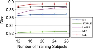
Segmentation performance as a function of the number of atlases used. [Color figure can be viewed in the online issue, which is available at http://wileyonlinelibrary.com.]
DISCUSSION AND CONCLUSION
In this study, we propose a local label learning (LLL) strategy for multi‐atlas based image segmentation. Instead of explicitly defining a weighting model to fuse the atlas labels, we utilize a machine learning method to build voxel‐wise classifiers based on image appearance and texture information. To get a robust classifier that generalizes well for each target voxel, we adopt a local patch strategy to get a training set with abundant appearance and texture information on which an L1‐regularized SVM classifier is built in conjunction with a kNN training sample selection strategy.
Our method has the following novelties. First, an L1‐regularized supervised learning method is utilized to learn the relationship between the segmentation label and image appearance/texture for each voxel. The supervised learning method can take rich information as input for learning a mapping from images to the segmentation label, and the adopted L1 SVM can handle the potential redundant information of image features. Besides the feature extraction method adopted in our method, other sophisticated feature extraction techniques can also be adopted in this framework [Dunn and Higgins, 1995]. Second, a local patch strategy is used to get a training set for each voxel to be segmented. Utilizing such a strategy to get the training set not only increases the number of training samples, but also minimizes the partial volume effect due to imaging resolution and the adverse effect of image registration errors. Finally, the kNN strategy based SVM classification is utilized to get a balanced training dataset. The kNN strategy has been demonstrated successful for learning problems with unbalanced training samples [Zhang et al., 2006].
The comparison results have demonstrated that our method could obtain better performance for segmenting images with different spatial resolutions than alternative state‐of‐the‐art methods. It is worth noting that a direct comparison of results across publications is difficult and can be affected by several factors, such as the segmentation protocol, the imaging protocol, and the patient population [Collins and Pruessner, 2010]. Since large labels might lead to larger overlap values in segmentation evaluation [Rohlfing et al., 2004a], multiple segmentation metrics should be used to comprehensively evaluate the segmentation results. One summary of the hippocampal segmentation performance reported in recent literature can be found in Table X of [Wang et al., 2011a]. Most of the recently published results had Dice index less than 0.9 and the method combining multi‐atlas‐based segmentation with an error correction step achieved the highest Dice index of 0.908 [Wang et al., 2011a]. We got a similar performance with the highest Dice index of 0.910 for images from subjects of mixed diagnostic groups of Alzheimer's disease. Our results have also indicated that the hippocampus segmentation performance is hinged on the spatial resolution of images to be segmented.
One recent study [Heckmann et al., 2011] has provided a publicly available repository of anatomically segmented brain images for the ADNI dataset. The segmentation results were also generated by a multi‐atlas based segmentation method [Heckemann et al., 2010]. Though hippocampal labels were available for these images, they were obtained with a segmentation protocol different from ours. We did not apply out method to the dataset with hippocampus labels provided by the study [Heckemann et al., 2011] for following reasons. First, our method is not suitable for segmenting hippocampus based on atlases labeled without the hippocampal tail. Since the hippocampal main body and tail have similar intensity information as shown in Figure 13, our method, achieving segmentation based on image intensity information, will generate results including the hippocampal tail. Our method cannot automatically cut the tail. Second, our method might not be able to effectively handle label errors of atlas. As shown in Figure 13, the segmentation results contained errors. Such segmentation label errors also make the performance evaluation complicated.
Figure 13.
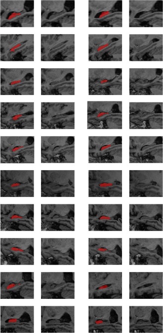
Ten randomly selected images and their segmentation labels of hippocampus obtained from the results provided by the study [Heckemann et al., 2011]. Each row shows one image's two slices and their corresponding segmentation labels. [Color figure can be viewed in the online issue, which is available at http://wileyonlinelibrary.com.]
One major issue of the multi‐atlas based image segmentation methods is their high computational cost, mainly due to the image registration. To reduce the computation cost of image registration, one can select a small number of atlases [Aljabar et al., 2009]. As demonstrated in our experiments, a small set of around 20 atlases could lead to a stable segmentation performance. Recent studies have proposed nonlocal patch‐based image labeling strategies with linear image registration based atlas alignment [Coupe et al., 2011; Rousseau et al., 2011]. However, such non‐local search procedures may increase the computational cost due to the reason that the computational cost of non‐local searching in the label fusion step might be higher than the computational cost of non‐rigid image registration, as pointed out in [Rousseau et al., 2011]. For speeding up the image registration and subsequently the image segmentation, it might be a good choice to use graphics processing units (GPUs) [Huang et al., 2011; Samant et al., 2008; Sharp et al., 2007] since a GPU‐based image registration can achieve a speedup of 25 times for atlas‐based brain image segmentation [Han et al., 2009]. In this study, we have implemented our algorithm using Matlab. It took about 7 min to fuse labels for segmenting one side of the hippocampi using single thread on a computation workstation (Intel xeonx5667) with CPUs of 3.07 GHZ.
The proposed method is designed for problems with two labels: foreground or background. However, it is straightforward to use our method in segmentation problems with multiple structures by iteratively segmenting one structure at a time. The method can also be extended for segmentation problems with multiple structures by replacing the two‐class SVM classifiers with multi‐class classifiers, such as random forests [Breiman, 2001]. Furthermore, if fuzzy label models such as those based on distance transforms are used, our method can also be extended by adopting regression techniques.
The proposed method could be further improved using the following strategies. First, shape regularization can be incorporated into the image segmentation framework. In this study, we performed voxel‐wise classification. We expect that smoother labels could be obtained by explicitly including shape constrains. Second, our algorithm could be extended to handle multiple brain structures with a multi‐class based supervised learning strategy.
ACKNOWLEDGMENTS
The study is coordinated by the Alzheimer's Disease Cooperative Study at the University of California, San Diego. ADNI data are disseminated by the Laboratory for Neuro Imaging at the University of California, Los Angeles.
This article was published online on 23 October 2014. An error was subsequently identified. This notice is included in the online and print versions to indicate that both have been corrected 28 February 2014.
REFERENCES
- Aljabar P, Heckeman R, Hammers A, Hajnal JV, Rueckert D (2007): Classifier selection strategies for label fusion using large atlas databases. Med Image Comput Comput Assist Interv 4791:523–531. [DOI] [PubMed] [Google Scholar]
- Aljabar P, Heckemann RA, Hammers A, Hajnal JV, Rueckert D (2009): Multi‐atlas based segmentation of brain images: Atlas selection and its effect on accuracy. Neuroimage 46:726–738. [DOI] [PubMed] [Google Scholar]
- Artaechevarria X, Munoz‐Barrutia A, Ortiz‐de‐Solorzano C (2008): Effleient classifier generation and weighted voting for aflas‐based segmentation: Two small steps faster and closer to the combination oracle. SPIE Med Imag 2008:6914. [Google Scholar]
- Artaechevarria X, Munoz‐Barrutia A, Ortiz‐de‐Solorzano C (2009): Combination strategies in multi‐atlas image segmentation: Application to brain MR data. IEEE Trans Image Process 28:1266–1277. [DOI] [PubMed] [Google Scholar]
- Ashburner J, Friston KJ (2005): Unified segmentation. Neuroimage 26:839–851. [DOI] [PubMed] [Google Scholar]
- Asman AJ, Landman BA (2011): Robust statistical label fusion through consensus level, labeler accuracy, and truth estimation (COLLATE). IEEE Trans Image Process 30:1779–1794. [DOI] [PMC free article] [PubMed] [Google Scholar]
- Asman AJ, Landman BA (2012): Non‐local STAPLE: An intensity‐driven multi‐atlas rater model. Med Image Comput Comput Assist Interv 15:426–434. [DOI] [PMC free article] [PubMed] [Google Scholar]
- Avants BB, Epstein CL, Grossman M, Gee JC (2008): Symmetric diffeomorphic image registration with cross‐correlation: Evaluating automated labeling of elderly and neurodegenerative brain. Med Image Anal 12:26–41. [DOI] [PMC free article] [PubMed] [Google Scholar]
- Avants BB, Yushkevich P, Pluta J, Minkoff D, Korczykowski M, Detre J, Gee JC (2010): The optimal template effect in hippocampus studies of diseased populations. Neuroimage 49:2457–2466. [DOI] [PMC free article] [PubMed] [Google Scholar]
- Bajcsy R, Lieberson R, Reivich M (1983): A computerized system for the elastic matching of deformed radiographic images to idealized atlas images. J Comput Assist Tomogr 7:618–625. [DOI] [PubMed] [Google Scholar]
- Breiman L (2001): Random forests. Mach Learn 45:5–32. [Google Scholar]
- Collins DL, Holmes CJ, Peters TM, Evans AC (1995): Automatic 3‐D model‐based neuroanatomical segmentation. Human Brain Mapp 3:190–208. [Google Scholar]
- Collins DL, Pruessner JC (2010): Towards accurate, automatic segmentation of the hippocampus and amygdala from MRI by augmenting ANIMAL with a template library and label fusion. Neuroimage 52:1355–1366. [DOI] [PubMed] [Google Scholar]
- Collins DL, Zijdenbos AP, Baare WFC, Evans AC (1999): ANIMAL+INSECT: Improved cortical structure segmentation. Inf Process Med Imaging 1613:210–223. [Google Scholar]
- Coupe P, Manjon JV, Fonov V, Pruessner J, Robles M, Collins DL (2011): Patch‐based segmentation using expert priors: Application to hippocampus and ventricle segmentation. Neuroimage 54:940–954. [DOI] [PubMed] [Google Scholar]
- Dunn D, Higgins WE (1995): Optimal Gabor filters for texture segmentation. IEEE Trans Image Process 4:947–964. [DOI] [PubMed] [Google Scholar]
- Eng J (2003): Sample size estimation: How many individuals should be studied? Radiology 227:309–313. [DOI] [PubMed] [Google Scholar]
- Fan RE, Chang KW, Hsieh CJ, Wang, XR , Lin CJ (2008): LIBLINEAR: A library for large linear classification. J Mach Learn Res 9:1871–1874. [Google Scholar]
- Fischl B, Salat DH, Busa E, Albert M, Dieterich M, Haselgrove C, van der Kouwe A, Killiany R, Kennedy D, Klaveness S, Montillo A, Makris N, Rosen B, Dale AM (2002): Whole brain segmentation: Automated labeling of neuroanatomical structures in the human brain. Neuron 33:341–355. [DOI] [PubMed] [Google Scholar]
- Fischl B, van der Kouwe A, Destrieux C, Halgren E, Segonne F, Salat DH, Busa E, Seidman LJ, Goldstein J, Kennedy D, Caviness V, Makris N, Rosen B, Dale AM (2004): Automatically parcellating the human cerebral cortex. Cereb Cortex 14:11–22. [DOI] [PubMed] [Google Scholar]
- Gee JC, Reivich M, Bajcsy R (1993): Elastically deforming 3D atlas to match anatomical brain images. J Comput Assist Tomogr 17:225–236. [DOI] [PubMed] [Google Scholar]
- Gering DT, Nabavi A, Kikinis R, Hata N, O'Donnell LJ, Grimson WE, Jolesz FA, Black PM, Wells WM III (2001): An integrated visualization system for surgical planning and guidance using image fusion and an open MR. J Magn Reson Imaging 13:967–975. [DOI] [PubMed] [Google Scholar]
- Hajnal JV, Xue H, Srinivasan L, Jiang SZ, Rutherford M, Edwards AD, Rueckert D (2007): Automatic segmentation and reconstruction of the cortex from neonatal MRI. Neuroimage 38:461–477. [DOI] [PubMed] [Google Scholar]
- Han X, Fischl B (2007): Atlas renormalization for improved brain MR image segmentation across scanner platforms. IEEE Trans Med Imaging 26:479–486. [DOI] [PubMed] [Google Scholar]
- Han X, Hibbard LS, Willcut V (2009): GPU‐accelerated, gradient‐free MI deformable registration for atlas‐based MR brain image segmentation. In: Proceedings of IEEE Conference on Computer Vision and Pattern Recognition (CVPR) Workshop, Miami, FL, pp 141–148.
- Hao Y, Liu J, Duan Y, Zhang X, Yu C, Jiang T, Fan Y (2012): Local label learning (L3) for multi‐atlas based segmentation SPIE Med Imaging 2012:8314.
- Heckemann RA, Hajnal JV, Aljabar P, Rueckert D, Hammers A (2006): Automatic anatomical brain MRI segmentation combining label propagation and decision fusion. Neuroimage 33:115–126. [DOI] [PubMed] [Google Scholar]
- Heckemann RA, Keihaninejad S, Aljabar P, Gray KR, Nielsen C, Rueckert D, Hajnal JV, Hammers A (2011): Automatic morphometry in Alzheimer's disease and mild cognitive impairment. Neuroimage 56:2024–2037. [DOI] [PMC free article] [PubMed] [Google Scholar]
- Heckemann R, Keihaninejad S, Aljabar P, Rueckert D, Hajnal JV, Hammers A (2010): Improving intersubject image registration using tissue‐class information benefits robustness and accuracy of multi‐atlas based anatomical segmentation. Neuroimage 51:221–227. [DOI] [PubMed] [Google Scholar]
- Huang TY, Tang YW, Ju SY (2011): Accelerating image registration of MRI by GPU‐based parallel computation. Magn Reson Imaging 29:712–716. [DOI] [PubMed] [Google Scholar]
- Iosifescu DV, Shenton ME, Warfield SK, Kikinis R, Dengler J, Jolesz FA, McCarley RW (1997): An automated registration algorithm for measuring MRI subcortical brain structures. Neuroimage 6:13–25. [DOI] [PubMed] [Google Scholar]
- Isgum I, Staring M, Rutten A, Prokop M, Viergever MA, van Ginneken B (2009): Multi‐atlas‐based segmentation with local decision fusion–Application to cardiac and aortic segmentation in CT scans. IEEE Trans Med Imaging 28:1000–1010. [DOI] [PubMed] [Google Scholar]
- Jack CR, Bernstein MA, Fox NC, Thompson P, Alexander G, Harvey D, Borowski B, Britson PJ, Whitwell JL, Ward C, Dale AM, Felmlee JP, Gunter JL, Hill DLG, Killiany R, Schuff N, Fox‐Bosetti S, Lin C, Studholme C, DeCarli CS, Krueger G, Ward HA, Metzger GJ, Scott KT, Mallozzi R, Blezek D, Levy J, Debbins JP, Fleisher AS, Albert M, Green R, Bartzokis G, Glover G, Mugler J, Weiner MW, Study A (2008): The Alzheimer's Disease Neuroimaging Initiative (ADNI): MRI methods. J Magn Reson Imaging 27:685–691. [DOI] [PMC free article] [PubMed] [Google Scholar]
- Jafari‐Khouzani K, Elisevich KV, Patel S, Soltanian‐Zadeh H (2011): Dataset of magnetic resonance images of nonepileptic subjects and temporal lobe epilepsy patients for validation of hippocampal segmentation techniques. Neuroinformatics 9:335–346. [DOI] [PMC free article] [PubMed] [Google Scholar]
- Jia H, Yap PT, Shen D (2012): Iterative multi‐atlas‐based multi‐image segmentation with tree‐based registration. Neuroimage 59:422–430. [DOI] [PMC free article] [PubMed] [Google Scholar]
- Jovicich J, Czanner S, Greve D, Haley E, van der Kouwe A, Gollub R, Kennedy D, Schmitt F, Brown G, MacFall J, Fischl B, Dale A (2006): Reliability in multi‐site structural MRI studies: Effects of gradient non‐linearity correction on phantom and human data. Neuroimage 30:436–443. [DOI] [PubMed] [Google Scholar]
- Khan AR, Cherbuin N, Wen W, Anstey KJ, Sachdev P, Beg MF (2011): Optimal weights for local multi‐atlas fusion using supervised learning and dynamic information (SuperDyn): Validation on hippocampus segmentation. Neuroimage 56:126–139. [DOI] [PubMed] [Google Scholar]
- Khan AR, Chung MK, Beg MF (2009): Robust atlas‐based brain segmentation using multi‐structure confidence‐weighted registration. Med Image Comput Comput Assist Interv 12:549–557. [DOI] [PubMed] [Google Scholar]
- Khan AR, Wang L, Beg MF (2008): FreeSurfer‐initiated fully‐automated subcortical brain segmentation in MRI using large deformation diffeomorphic metric mapping. Neuroimage 41:735–746. [DOI] [PMC free article] [PubMed] [Google Scholar]
- Kittler J, Hatef M, Duin RPW, Matas J (1998): On combining classifiers. IEEE Trans Pattern Anal Mach Intell 20:226–239. [Google Scholar]
- Langerak TR, van der Heide UA, Kotte AN, Viergever MA, van Vulpen M, Pluim JP (2010): Label fusion in atlas‐based segmentation using a selective and iterative method for performance level estimation (SIMPLE). IEEE Trans Image Process 29:2000–2008. [DOI] [PubMed] [Google Scholar]
- Leung KK, Barnes J, Modat M, Ridgway GR, Bartlett JW, Fox NC, Ourselin S, Initia ADN (2011): Brain MAPS: An automated, accurate and robust brain extraction technique using a template library. Neuroimage 55:1091–1108. [DOI] [PMC free article] [PubMed] [Google Scholar]
- Leung KK, Barnes J, Ridgway GR, Bartlett JW, Clarkson MJ, Macdonald K, Schuff N, Fox NC, Ourselin S (2010): Automated cross‐sectional and longitudinal hippocampal volume measurement in mild cognitive impairment and Alzheimer's disease. Neuroimage 51:1345–1359. [DOI] [PMC free article] [PubMed] [Google Scholar]
- Leventon ME, Grimson WEL, Faugeras O (2000): Statistical shape influence in geodesic active contours. In: Proceedings of IEEE Conference on Computer Vision and Pattern Recognition (CVPR), Volume 1, Hilton Head Island, SC, pp. 316–323.
- Lotjonen JMP, Wolz R, Koikkalainen JR, Thurfjell L, Waldemar G, Soininen H, Rueckert D, Initi ASDN (2010): Fast and robust multi‐atlas segmentation of brain magnetic resonance images. Neuroimage 49:2352–2365. [DOI] [PubMed] [Google Scholar]
- Magnotta VA, Heckel D, Andreasen NC, Cizadlo T, Corson PW, Ehrhardt JC, Yuh WT (1999): Measurement of brain structures with artificial neural networks: Two‐ and three‐dimensional applications. Radiology 211:781–790. [DOI] [PubMed] [Google Scholar]
- Marroquin JL, Santana EA, Botello S (2003) Hidden Markov measure field models for image segmentation. IEEE Trans Pattern Anal Mach Intell 25:1380–1387. [Google Scholar]
- Mazziotta JC, Valentino D, Grafton S, Bookstein F, Pelizzari C, Chen G, Toga AW (1991): Relating structure to function in vivo with tomographic imaging. Proc Ciba Found Symp 163:93–112. [DOI] [PubMed] [Google Scholar]
- Morra JH, Tu Z, Apostolova LG, Green AE, Avedissian C, Madsen SK, Parikshak N, Toga AW, Jack CR, Schuff N, Weiner MW, Thompson PM, Initi ASDN (2009a): Automated mapping of hippocampal atrophy in 1‐year repeat MRI data from 490 subjects with Alzheimer's disease, mild cognitive impairment, and elderly controls. Neuroimage 45:S3–S15. [DOI] [PMC free article] [PubMed] [Google Scholar]
- Morra JH, Tu Z, Apostolova LG, Green AE, Toga AW, Thompson PM (2010): Comparison of AdaBoost and support vector machines for detecting Alzheimer's disease through automated hippocampal segmentation. IEEE Trans Med Imaging 29:30–43. [DOI] [PMC free article] [PubMed] [Google Scholar]
- Morra JH, Tu ZW, Apostolova LG, Green AE, Avedissian C, Madsen SK, Parikshak N, Hua X, Toga AW, Jack CR, Weiner MW, Thompson PM (2009b): Validation of a fully automated 3D hippocampal segmentation method using subjects with Alzheimer's disease, mild cognitive impairment, and elderly controls. Neuroimage 44:1439–1439. [DOI] [PMC free article] [PubMed] [Google Scholar]
- Ostby Y, Tamnes CK, Fjell AM, Westlye LT, Due‐Tonnessen P, Walhovd KB (2009): Heterogeneity in subcortical brain development: A structural magnetic resonance imaging study of brain maturation from 8 to 30 years. J Neurosci 29:11772–11782. [DOI] [PMC free article] [PubMed] [Google Scholar]
- Pierson R, Corson PW, Sears LL, Alicata D, Magnotta V, Oleary D, Andreasen NC (2002): Manual and semiautomated measurement of cerebellar subregions on MR images. Neuroimage 17:61–76. [DOI] [PubMed] [Google Scholar]
- Pohl KM, Fisher J, Grimson WE, Kikinis R, Wells, W.M (2006a): A Bayesian model for joint segmentation and registration. Neuroimage 31:228–239. [DOI] [PubMed] [Google Scholar]
- Pohl KM, Fisher J, Shenton M, McCarley RW, Grimson WE, Kikinis R, Wells WM (2006b): Logarithm odds maps for shape representation. Med Image Comput Comput Assist Interv 9:955–963. [DOI] [PMC free article] [PubMed] [Google Scholar]
- Powell S, Magnotta VA, Johnson H, Jammalamadaka VK, Pierson R, Andreasen NC (2008): Registration and machine learning‐based automated segmentation of subcortical and cerebellar brain structures. Neuroimage 39:238–247. [DOI] [PMC free article] [PubMed] [Google Scholar]
- Rohlfing T, Brandt R, Menzel R, Maurer CR Jr (2004a): Evaluation of atlas selection strategies for atlas‐based image segmentation with application to confocal microscopy images of bee brains. Neuroimage 21:1428–1442. [DOI] [PubMed] [Google Scholar]
- Rohlfing T, Maurer CR (2007): Shape‐based averaging. IEEE Trans Med Imaging 16:153–161. [DOI] [PubMed] [Google Scholar]
- Rohlfing T, Russakoff DB, Maurer CR Jr (2004b): Performance‐based classifier combination in atlas‐based image segmentation using expectation‐maximization parameter estimation. IEEE Trans Med Imaging 23:983–994. [DOI] [PubMed] [Google Scholar]
- Rousseau F, Habas PA, Studholme C (2011): A supervised patch‐based approach for human brain labeling. IEEE Trans Med Imaging 30:1852–1862. [DOI] [PMC free article] [PubMed] [Google Scholar]
- Sabuncu MR, Yeo BT, Van Leemput K, Fischl B, Golland, P (2010): A generative model for image segmentation based on label fusion. IEEE Trans Med Imaging 29:1714–1729. [DOI] [PMC free article] [PubMed] [Google Scholar]
- Samant SS, Xia J, Muyan‐Ozcelik P, Owens JD (2008): High performance computing for deformable image registration: Towards a new paradigm in adaptive radiotherapy. Med Phys 35:3546–3553. [DOI] [PubMed] [Google Scholar]
- Schuff N, Woerner N, Boreta L, Kornfield T, Shaw LM, Trojanowski JQ, Thompson PM, Jack CR, Weiner MW, Initi ASDN (2009): MRI of hippocampal volume loss in early Alzheimers disease in relation to ApoE genotype and biomarkers. Brain 132:1067–1077. [DOI] [PMC free article] [PubMed] [Google Scholar]
- Sdika M (2010): Combining atlas based segmentation and intensity classification with nearest neighbor transform and accuracy weighted vote. Med Image Anal 14:219–226. [DOI] [PubMed] [Google Scholar]
- Sharp GC, Kandasamy N, Singh H, Folkert M (2007): GPU‐based streaming architectures for fast cone‐beam CT image reconstruction and demons deformable registration. Phys Med Biol 52:5771–5783. [DOI] [PubMed] [Google Scholar]
- Sled JG, Zijdenbos AP, Evans AC (1998): A nonparametric method for automatic correction of intensity nonuniformity in MRI data. IEEE Trans Med Imaging 17:87–97. [DOI] [PubMed] [Google Scholar]
- Sowell ER, Trauner DA, Gamst A, Jernigan TL (2002): Development of cortical and subcortical brain structures in childhood and adolescence: A structural MRI study. Dev Med Child Neurol 44:4–16. [DOI] [PubMed] [Google Scholar]
- Spinks R, Magnotta VA, Andreasen NC, Albright KC, Ziebell S, Nopoulos P, Cassell M (2002): Manual and automated measurement of the whole thalamus and mediodorsal nucleus using magnetic resonance imaging. Neuroimage 17:631–642. [PubMed] [Google Scholar]
- Toriwaki J, Yoshida H (2009): Fundamentals of Three‐Dimensional Digital Image Processing. London: Springer. [Google Scholar]
- Tu Z, Narr KL, Dollar P, Dinov I, Thompson PM, Toga AW (2008): Brain anatomical structure segmentation by hybrid discriminative/generative models. IEEE Trans Med Imaging 27:495–508. [DOI] [PMC free article] [PubMed] [Google Scholar]
- Tu Z, Toga AW (2007): Towards whole brain segmentation by a hybrid model. Med Image Comput Comput Assist Interv 10:169–177. [DOI] [PubMed] [Google Scholar]
- Twining CJ, Cootes T, Marsland S, Petrovic V, Schestowitz R, Taylor CJ (2005): A unified information‐theoretic approach to groupwise non‐rigid registration and model building. Inf Process Med Imaging 3565:1–14. [DOI] [PubMed] [Google Scholar]
- van Rikxoort EM, Isgum I, Arzhaeva Y, Staring M, Klein S, Viergever MA, Pluim JPW, van Ginneken B (2010): Adaptive local multi‐atlas segmentation: Application to the heart and the caudate nucleus. Med Image Anal 14:39–49. [DOI] [PubMed] [Google Scholar]
- Wang H, Das SR, Suh JW, Altinay M, Pluta J, Craige C, Avants B, Yushkevich PA (2011a): A learning‐based wrapper method to correct systematic errors in automatic image segmentation: Consistently improved performance in hippocampus, cortex and brain segmentation. Neuroimage 55:968–985. [DOI] [PMC free article] [PubMed] [Google Scholar]
- Wang H, Suh JW, Das S, Pluta J, Altinay M, Yushkevich P (2011b): Regression‐based label fusion for multi‐atlas segmentation. In: Proceedings of IEEE Conference on Computer Vision and Pattern Recognition (CVPR), Providence, RI, pp 1113–1120. [DOI] [PMC free article] [PubMed]
- Warfield SK, Zou KH, Wells WM (2004): Simultaneous truth and performance level estimation (STAPLE): An algorithm for the validation of image segmentation. IEEE Trans Med Imaging 23:903–921. [DOI] [PMC free article] [PubMed] [Google Scholar]
- Wolz R, Aljabar P, Hajnal JV, Hammers A, Rueckert D (2010a): LEAP: Learning embeddings for atlas propagation. Neuroimage 49:1316–1325. [DOI] [PMC free article] [PubMed] [Google Scholar]
- Wolz R, Heckemann RA, Aljabar P, Hajnal JV, Hammers A, Lotjonen J, Rueckert D, Initi ASDN (2010b): Measurement of hippocampal atrophy using 4D graph‐cut segmentation: Application to ADNI. Neuroimage 52:109–118. [DOI] [PubMed] [Google Scholar]
- Wu MJ, Rosano C, Lopez‐Garcia P, Carter CS, Aizenstein HJ (2007): Optimum template selection for atlas‐based segmentation. Neuroimage 34:1612–1618. [DOI] [PubMed] [Google Scholar]
- Yeo BT, Sabuncu M., Desikan R, Fischl B, Golland P (2008): Effects of registration regularization and atlas sharpness on segmentation accuracy. Med Image Anal 12:603–615. [DOI] [PMC free article] [PubMed] [Google Scholar]
- Yuan GX, Chang KW, Hsieh CJ, Lin C.J (2010): A comparison of optimization methods and software for large‐scale L1‐regularized linear classification. J Mach Learn Res 11:3183–3234. [Google Scholar]
- Zhang H, Berg AC, Maire M, Malik J (2006): SVM‐KNN: Discriminative nearest neighbor classification for visual category recognition. Comput Vis Pattern Recognit 2006:2126–2136. [Google Scholar]