Predictors of coupling between structural and functional cortical networks in normal aging

Abstract

Understanding how the mammalian neocortex creates cognition largely depends on knowledge about large‐scale cortical organization. Accumulated evidence has illuminated cortical substrates of cognition across the lifespan, but how topological properties of cortical networks support structure‐function relationships in normal aging remains an open question. Here we investigate the role of connections (i.e., short/long and direct/indirect) and node properties (i.e., centrality and modularity) in predicting functional‐structural connectivity coupling in healthy elderly subjects. Connectivity networks were derived from correlations of cortical thickness and cortical glucose consumption in resting state. Local‐direct connections (i.e., nodes separated by less than 30 mm) and node modularity (i.e., a set of nodes highly interconnected within a topological community and sparsely interconnected with nodes from other modules) in the functional network were identified as the main determinants of coupling between cortical networks, suggesting that the structural network in aging is mainly constrained by functional topological properties involved in the segregation of information, likely due to aging‐related deficits in functional integration. This hypothesis is supported by an enhanced connectivity between cortical regions of different resting‐state networks involved in sensorimotor and memory functions in detrimental to associations between fronto‐parietal regions supporting executive processes. Taken collectively, these findings open new avenues to identify aging‐related failures in the anatomo‐functional organization of the neocortical mantle, and might contribute to early detection of prevalent neurodegenerative conditions occurring in the late life. Hum Brain Mapp 35:2724–2740, 2014. © 2013 Wiley Periodicals, Inc.

INTRODUCTION

A central goal in systems neuroscience is to unveil how cognitive abilities result from dynamic interactions in large‐scale cortical networks, and to further identify how development, aging and brain diseases contribute to reshaping this complex organization. The notion that structural networks represent the physical substrate of functional connectivity patterns in the human brain has received considerable attention over the last few years [Cohen et al., 2008; Greicius et al., 2009; Koch et al., 2002; Van den Heuvel et al., 2009]. This relationship is reinforced with cerebral maturation [Hagmann et al., 2010], suggesting that associations between structural and functional connectivity (in the next, functional‐structural coupling or F‐S coupling) play a role in creating patterns of neural synchronization in the human brain.

The assumption that cortical structure and functional dynamics are intrinsically related has been supported by experiments showing a good correspondence between structural and functional hubs (i.e., cortical nodes massively connected to other nodes) at multiple temporal scales [Honey et al., 2007]. But the strength, persistence, and spatial distribution of functional connectivity patterns are not only constrained by node attributes but also by connection features. In this line, Honey et al. [2009] showed that direct structural links based on diffusion tensor image (DTI) tractography were excellent predictors of the resting‐state functional connectivity network. However, this study also revealed that indirect structural connections (i.e., pairs of nodes not directly connected to one another) also contributed moderately to functional connectivity patterns [Honey et al., 2009].

Accumulated evidence has strengthened the idea that intrinsic features of nodes and node connectivity constraint topological organization of functional networks, but it remains unknown whether such influence depends on the connection distance. This aspect becomes especially relevant in aging since both structural and functional hubs overlap heteromodal association areas in prefrontal and posterior parietal cortices [Honey et al., 2007], the late‐maturing cortical territories most vulnerable to aging‐related loss of structural integrity [McGinnis et al., 2011]. In fact, these cortical regions not only exhibit greater shrinkage [e.g., Raz et al., 2005], thinning [e.g., Fjell et al., 2009] and white‐matter atrophy [e.g., Jeon et al., 2012] with aging, but they are also involved in cognitive capacities affected by aging like attention, executive function, and cognitive control [e.g., Gazzaley and D'Esposito, 2007]. In this line, evidence has shown that older brains benefit from larger areas of activation in the prefrontal and posterior cingulate cortices, likely revealing neural compensatory mechanisms [Batouli et al., 2009].

As these cortical regions are not monosynaptically connected, one would expect less similarity between structural and functional networks (i.e., less F‐S coupling) when considering cortical nodes linked through long‐distance connections. Here we systematically tested this hypothesis by examining to what extent morphometric (cortical thickness) and functional (cortical glucose consumption) correlations between cortical regions (nodes) separated by either short (≤30 mm, local connections) or long distances (>30 mm, global connections) govern the relationship between structural and functional connectivity networks in normal aging. We hypothesize that highly interconnected nodes communicated through short connections (i.e., local hubs) like those corresponding to sensory/motor and unimodal association areas, which are less affected by aging [McGinnis et al., 2011], should predict better F‐S coupling than those highly interconnected nodes overlapping cortical heteromodal association areas whose communication relies on distant connections (i.e., global hubs).

Functional and structural cerebral connectivity graphs have been commonly derived from functional magnetic resonance imaging (fMRI) and diffusion tensor imaging (DTI) tractography, respectively [e.g., Honey et al., 2009; Supekar et al., 2010; Van den Heuvel et al., 2009]. The ability of DTI‐based techniques to successfully estimate cerebral anatomical connections critically depends on both fiber length and the underlying anatomical complexity. Whereas long anatomical pathways connecting distant cortical territories can be reliably determined with conventional DTI tractography [Oishi et al., 2008], short association fibers (also referred to as U‐fibers) connecting adjacent gyri and mediating communication between association areas are hardly detectable with this technique [Oishi et al., 2011]. Therefore, considering association fibers derived from DTI‐based models in cortical network analysis might lead to oversimplification of reality [Oishi et al., 2011]. Alternatively, topological properties of cortical networks based on thickness measurements have recently provided novel insights into the organizational principles of the human brain [Bassett et al., 2008; Chen et al., 2008; He et al., 2007; Lv et al., 2010]. Although the biological substrate of correlated cortical thickness is still poorly understood [Chen et al., 2011], connectivity patterns derived from thickness correlations have shown to be relatively consistent with those derived from DTI [Lerch et al., 2006]. Furthermore, physiological mechanisms underlying blood oxygenation level‐dependent (BOLD) responses are markedly different from those responsible for cerebral glucose consumption, likely revealing different aspects of functional cortical networks (see SM1 in Supporting Information for physiological differences between cerebral BOLD responses and FDG‐PET).

By using MRI‐cortical thickness and FDG‐PET cortical maps of glucose consumption, we further investigated whether F‐S coupling was similarly predicted by structural and functional connections in healthy elderly subjects. This prediction was supported not only by the high correspondence between the two‐modality networks found in previous studies [Honey et al., 2007; Van den Heuvel et al., 2008], but also by previous evidence showing that function can be inferred from structure [Honey et al., 2009] and vice versa [Greicius et al., 2009]. To this aim, we considered all nodes integrated within the cortical network, those nodes showing either high degree/betweenness centrality (i.e., hubs), and nodes relevant within modules, a network characteristic related to segregation of information [Schwarz et al., 2008]. As effects of aging are more noticeable on network integration (i.e., centrality measures) than on network segregation (i.e., modularity) [Chen et al., 2011], topological properties supporting segregation should significantly enhance prediction of F‐S coupling in normal aging.

MATERIALS AND METHODS

Subjects

Thirty cognitively intact elderly volunteers (66.4 ± 5.1 years [mean ± standard deviation], 17 females; Mini Mental State Examination: 28.4 ± 0.2) were enrolled in the study. This experiment received Institutional ethics approval by the Ethical Committee for Human Research at the University Pablo de Olavide, and written informed consent was obtained from each participant.

Inclusion criteria were (i) no subjective memory complaints or objective memory impairment corroborated by neuropsychological assessment, (ii) Global Clinical Dementia Rating (CDR) score of 0 (no dementia), and (iii) normal independent function judged clinically and by means of a standardized scale for the activities of daily living (IDDD). None of them reported a history of neurological, psychiatric disorders and/or major medical illness.

MRI Acquisition

Structural MRI was performed on a whole‐body Philips Intera 1.5T MRI scanner (Philips, The Netherlands) equipped with an 8‐channel head coil. Two concomitant high‐resolution MP‐RAGE (magnetization‐prepared rapid gradient echo) T1‐weighted cerebral scans were obtained from each participant. The two cerebral images were further averaged after motion correction to enhance the signal‐to‐noise ratio. Acquisition parameters were empirically optimized for grey/white matter contrast (repetition time = 2,300 ms, echo‐time = 4 ms, flip angle = 8°, matrix dimensions 256 × 192, 184 contiguous sagittal 1.2 mm thick slices, time per acquisition = 5.4 min).

FDG‐PET Acquisition and Preprocessing

FDG‐PET cerebral images were acquired on a whole‐body PET‐TAC Siemens Biograph 16 HiREZ scanner (Siemens Medical Systems, Germany) with in‐plane and axial resolution of 4.2 and 4.5 mm full‐width at half maximum (FWHM), respectively. Subjects fasted for at least 8 h before PET examination. Intravenous lines were placed 10 to 15 min before tracer injection of a mean dose of 370 MBq of 2‐[18F]fluoro‐2‐deoxy‐d‐glucose (FDG). Participants stayed in a dimly lighted room with their eyes closed to minimize external stimuli during the FDG uptake period. PET scans lasted approximately 30 min after the FDG injection. A transmission scan was used for attenuation correction, and cerebral FDG‐PET scans were reconstructed with 2.6 × 2.6 × 2 mm voxel resolution by using standard two‐dimensional back projection filters. We applied partial volume correction (PVC) to cerebral FDG‐PET images with the algorithm implemented in the PMOD software v3.17 (available at: http://www.pmod.com) [Giovacchini et al., 2004]:

$$C_{gm}=\left(C-C_{wm}\ast S_{wm}\right)/S_{gm}$$

where $C_{gm}$ refers to the corrected glucose consumption in each gray matter (GM) voxel after PVC, C denotes the uncorrected activity, $C_{wm}$ is the estimated white matter (WM) activity (assumed to be homogeneous), $S_{wm}$ is the smoothed WM mask, and $S_{gm}$ corresponds to the smoothed GM mask.

Cerebral MRI scans were registered to the Talairach stereotaxic space and then co‐registered to FDG‐PET brain images. The co‐registration algorithm implemented in PMOD applies rigid transformations (rotations and translations) to maximize mutual information between anatomical and functional brain features, thus enhancing spatial localization of cerebral glucose consumption. The analysis pipeline for estimating values of glucose consumption from cerebral FDG‐PET images is illustrated in Figure 1A (right panel).

Figure 1.

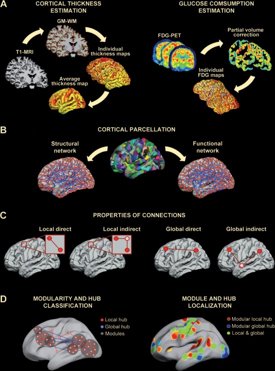
Analysis pipeline followed in this study. A. Cortical thickness estimation (left panel). T1‐MR images were segmented with Freesurfer to obtain individual cortical thickness maps that were further averaged to establish the cortical parcellation scheme. Cortical glucose consumption estimation (right panel). Partial volume effects were corrected on individual FDG‐PET cerebral images to obtain glucose consumption maps. B. Cortical parcellation. By applying a backtracking algorithm [Romero‐Garcia et al., 2012], the cortical surface was divided into 599 regions (with a surface area of 250 mm² each). Structural and functional cortical networks were based on thickness and glucose consumption, respectively, and adjacency matrices were obtained from this cortical scheme. C. Properties of connections. We calculated separately the influence of different structural connections (local direct, local indirect, global direct, and global indirect) on F‐S coupling for all network nodes, hubs (based on node degree and betweenness), and cortical regions grouped into modules. D. Left panel. Schematic representation of different types of hubs (local and global) and network modules (classification criteria are detailed in Materials and Methods). Right panel. Example of regional distribution of modular hubs in cortical networks. The color scale represents the proportion of sparsities for one specific region that reached the hub criterion.

Cortical Surface Reconstruction and Cortical Thickness Estimation

Both cortical surface reconstruction and cortical thickness estimation were performed with Freesurfer v5.1 (available at: http://surfer.nmr.mgh.harvard.edu/) following standardized analysis protocols. Pial/white matter boundaries were enhanced by manual editing, thus increasing the reliability of cortical thickness measures. The cortical thickness analysis pipeline is illustrated in Figure 1A (left panel). Further details about cortical thickness estimations can be found in the Supporting Information (SM2).

Building Structural and Functional Cortical Networks

Cortical parcellation

Different cerebral scales lead to brain networks with different levels of small‐world organization [Romero‐Garcia et al., 2012; Sanabria‐Diaz et al., 2010; Van Wijk et al., 2010]. We employed here a cortical scheme comprised of 599 regions (each region with a surface area of 250 mm²) obtained with a backtracking algorithm. This cortical scheme has provided the best trade‐off between small‐world attributes of thickness‐based cortical networks and the number of cortical regions embedded in the scale; it has shown more resilience to targeted attacks than an atlas‐based scheme [Desikan‐Killiany atlas, 66 regions; Desikan‐Killiany et al., 2006]; and its network resilience was comparable to that derived from a highly grained cortical scale (1,494 regions) [Romero‐Garcia et al., 2012]. Figure 1B illustrates the cortical scheme used in the present study.

Structural and functional connectivity matrices

Morphometric‐based correlations have been commonly used to establish connectivity patterns in structural network derived from neuroimaging datasets [Bassett et al., 2008; Chen et al., 2008; Fan et al., 2011; He et al., 2007; Lv et al., 2010; Sanabria‐Diaz et al., 2010]. In this study, structural and functional cortical networks were built from partial correlations of interregional cortical thickness and cortical glucose consumption values, respectively (a schematic representation of this procedure is displayed in Fig. 1B). Effects of age, gender, age‐gender interaction, mean overall cortical thickness, and mean overall FDG consumption were removed by applying a linear regression analysis across cortical regions.

Cortical networks are typically inferred from neuroimaging datasets with fewer subjects than cortical regions [e.g., Fan et al., 2011; Hänggi et al., 2011]. This experimental setting, known as the “small n, large p” problem, leads to both inaccurate estimations of the regression coefficients and overfitted models that result in inflated mean square errors during model validation [Peng et al., 2009]. To counteract this drawback, we applied a regularization method based on the Ledoit‐Wolf lemma that shrinks the covariance estimates [Opgen‐Rhein et al., 2007]. This method results in a more accurate, well‐conditioned and positive‐definite covariance matrix [Schäfer and Strimmer, 2005]. Corrected covariance is hence invertible and the partial correlation can be computed as:

$$r_{i,j}=-S_{i,j}^{-1}/\sqrt{S_{i,i}^{-1}\times S_{j,j}^{-1}}$$

where $r_{i,j}$ is the partial correlation between region i and region j, and $S_{i,j}^{-1}$ represents the {i,j}_th element of the inverted covariance matrix $S^{-1}$. Partial correlations computed from all possible pairs {i,j} of cortical regions result in a matrix of p rows by p columns (where p is the number of regions) containing the strength of the relationships (i.e., connection weight) among cortical regions included in the parcellation scheme.

Adjacency matrices and sparsity

The partial correlation matrix was restricted to positive values in each cortical network and further binarized using a wide range of sparsities (from 1 to 20%). Sparsities above 20% were disregarded because they result in random graphs [Bassett et al., 2008; Fan et al., 2011; Romero‐Garcia et al., 2012]. This approach, although largely used for the estimation of morphometric connectivity [He et al., 2009; Tijms et al., 2012; Wu et al., 2012], neglects the role of anti‐correlated nodes (negative correlations) on network organization [Blumenfeld et al., 2004]. Accordingly, cortical networks were also built taking into account absolute values of both negative and positive partial correlations [Bernhardt et al., 2011; He et al., 2008].

Determining small‐world properties in structural and functional cortical networks

Small‐world networks are characterized by a high density of local connections together with a scarce number of links between distant regions. This topological organization results in highly efficient networks with a relatively low wiring cost and optimal adaptability to a broad range of circumstances [Travers and Milgram, 1969]. Local connectivity was computed with the clustering coefficient (C _p) introduced by Soffer and Vazquez [2005]. This coefficient removes the correlation of the node degree present in the original C _p metric [Watts and Strogatz, 1998]:

$$C_p=\frac{{\displaystyle \sum _i{t}_i}}{{\displaystyle \sum _i{\Omega }_i}}$$

where $t_i$ is the number of connections among neighbours of the i node, and Ω_i represents the maximum possible number of connections between neighbours if i is limited by each neighbour degree. Ω_i is defined as:

$${\Omega }_i=\lfloor \frac{1}{2}{\displaystyle \sum _{neighbours}\left[\min \left(k_i,k_j\right)-1\right]}\rfloor$$

where k_i is the degree of the i node, and k_j is the degree of each neighbour of i [Soffer and Vazquez, 2005].

The global connectivity of the cortical network was determined with the path length metric (L _p). L _p denotes the average number of connections for the shortest path between every pair of regions [Watts and Strogatz, 1998]:

$$L_p=\frac{1}{n\left(n-1\right)}{\displaystyle \sum _{i\ne j}^n{d}_{ij}}$$

where n is the number of regions and $d_{ij}$ denotes the length of the shortest path between regions i and j. Shorter path lengths are associated with enhanced network capabilities to integrate information [Watts and Strogatz, 1998]. Small‐world properties are strongly influenced by intrinsic features of the network, such as the number of nodes, the number of connections, and the degree distribution. To counteract these effects, 100 random networks were built by using a random rewiring process [Maslov and Sneppen, 2002]. Thus, C _p and L _p of the cortical network were compared with the same metrices estimated in these 100 random networks. This resulted in a normalized clustering coefficient ${\gamma }_g=C_p/C_{rand}\gg 1$ and a normalized path length ${\lambda }_g=L_p/L_{rand}\approx 1$. The small‐worldness of a network combines both local and global properties in a unique descriptor (σ) that is defined as the ratio between the normalized clustering coefficient and the normalized path length ( $\sigma ={\gamma }_g/{\lambda }_g$). The above small‐world properties were computed for cortical networks derived from both positive partial correlations and from absolute values of positive and negative partial correlations.

Estimation of F‐S Coupling for Different Network Attributes

Pearson's correlation coefficient was employed to determine F‐S coupling [Hagmann et al., 2010; Honey et al., 2009; Skudlarski et al., 2010; Van den Heuvel et al., 2009; Zhang et al., 2011]. Levels of F‐S coupling were obtained from correlations between the partial correlation matrix of cortical thickness (structural connectivity) and the partial correlation matrix of cortical glucose consumption (functional connectivity). F‐S coupling was separately assessed for different types of connections (direct vs. indirect) and spatial scales (local vs. global). For direct coupling, correlations were constrained to those cortical regions considered as connected in the adjacency matrix. Coupling for indirect connections was computed considering the connectivity strength between pairs of regions resulting from the sum of all multiplicatively structural paths [Honey et al., 2009]:

$$\text{indirect}{\text{CS}}_{ij}={\displaystyle \sum _{\begin{array}{l}i\ne k\\ j\ne k\end{array}}{r}_{ik}}\cdot r_{kj}$$

where indirect CS_ij represents the strength of the indirect connection between regions i and j, k refers to each region directly connected to regions i and j, r_ik is the partial correlation between regions i and k, and r_kj denotes the partial correlation between regions k and j.

We regressed out the Euclidean distance from both direct and indirect connections [Honey et al., 2009]. Residuals resulting from regressing the functional correlations on distance were considered at examining levels of F‐S coupling. The Euclidean distance between centroids of two nodes was calculated by using the mean Talairach coordinates of voxels comprising each node [Honey et al., 2009]. Interhemispheric distances were computed assuming anatomical connections through callosal fibers:

$$InterDist(x,y)=\parallel x-CC{\parallel }^2+\parallel y-CC{\parallel }^2$$

where InterDist(x,y) refers to the interhemispheric distance between a region located in the x coordinate of the left hemisphere and another region located in the y coordinate of the right hemisphere, whereas CC corresponds to coordinates of the centroid of the corpus callosum.

Estimation of Node Centrality and Modularity in Structural and Functional Networks

Centrality reveals the importance of a node within the network [Langer et al., 2012]. This network property can be measured with different metrics, each one describing different aspects of hubs. One possibility is to use the node degree (D_i) that considers the total number of connections for each region. By using this metric, hubs were classified into four categories (Fig. 1C). Local direct hubs were defined as cortical regions with a node degree above the mean plus the standard deviation within 30 mm of a neighborhood area. Global direct hubs were similarly defined for connections longer than 30 mm. Hubs supported by indirect connections were assigned to regions with the highest number of nodes not directly connected, but with at least one two‐edge path connecting them. These nodes were considered local if the sum of the shortest paths of two connections below 30 mm was above the mean plus the standard deviation, whereas nodes were classified as global if connections were greater than 30 mm. We next computed the probability of each type of hub as the number of sparsities in which one specific node reached the hub condition (the mean plus the standard deviation) divided by the total number of sparsities (Fig. 1D, left panel).

Hubs based on node degree neglect those nodes acting as relevant relay stations within the cortical network [Zhang et al., 2011], aspect taken into account by the betweenness centrality. The betweenness of a node i is defined as the number of shortest paths between any two nodes that run through node i [Freeman, 1977]. Given that this centrality measure does not allow classifying hubs according to direct/indirect connections, we computed the betweenness centrality for local and global nodes separately, and next, estimated the F‐S coupling (see section below) for those nodes with betweenness above the mean plus one standard deviation and whose connections were either direct or indirect.

To determine cortical nodes organized into modules, we applied the hierarchical clustering criterion defined by Ferrarini et al. [2009]. This procedure groups nodes on a dendrogram by using the cluster coefficient criterion of Soffer and Vazquez [2005] as a function of distance. Distance between two nodes was defined as:

$$d_{A,B}=1-clus\left(A,B\right)$$

where clus (A,B) refers to the C _p for a pair of nodes (A and B) computed as the C _p of an auxiliary node H supposedly connected to A and B and to all their direct neighbors. The larger the number of connections between A and B, the higher the probability of being included within the same module by the hierarchical clustering procedure [Ferrarini et al., 2009]. This definition of modularity takes into account overlapping and inclusive relationships among modules, and has proved to be more specific than other approaches in discriminating different cluster topologies in brain networks [Ferrarini et al., 2009]. Those nodes with a large amount of shared connections (grouped by the hierarchical dendrogram on the basis of its high clus (A,B)) were considered as modular in the current study, and their connections to other nodes were next used to determine levels of F‐S coupling. Since this definition of modularity does not provide information about local and global network properties, we further quantified how many local and global hubs (determined with the node degree) overlapped modular nodes above 40% of sparsities (Fig. 1D, right panel).

Estimation of F‐S Coupling for Different Connection Properties

F‐S coupling based on direct and indirect connections was computed among nodes separated by Euclidean distances below (local) or above 30 mm (global), considering all nodes comprising the cortical network, nodes with either high degree or betweenness centrality (hubs), and nodes with high modularity. This analysis was performed over a broad sparsity range (from the first one at which the network is fully connected up to 20%). Significance of F‐S coupling was determined by applying nonparametric permutation tests (p < 0.05). Firstly, correlations were computed for every randomization (n = 10,000) of either structural or functional connections, and next the 95th quantile of the resulting distribution was used as a statistical threshold to retain or reject the null hypothesis of no significant relationship between functional and structural connectivity networks.

To compare results derived from different node attributes (all nodes, node degree, betweenness, and modularity) for each type of connectivity variant (local direct, local indirect, global direct, global indirect), we applied a bootstrapping method that kept constant the number of r‐values used to compute the F‐S coupling across node attributes and sparsities. F‐S coupling was computed in 10,000 equal‐size subsets of r‐values randomly selected for each node attribute and sparsity. Next, differences between pairs of node attributes were evaluated with t‐tests for independent samples across sparsities. Finally, permutation testing was used to establish the statistical significance of these differences. In particular, F‐S coupling values were permutated 10,000 times between condition pairs (all nodes vs. the two measures of centrality, all nodes vs. modules, modules vs. the two measures of centrality, and node degree vs. betweenness). For every condition pair and permutation, we computed the t statistic for each sparsity level and selected the highest value. The 95th quantile of this randomized distribution of maximum t statistics was used as a critical value to retain or reject the null hypothesis of no differences between node attributes. This procedure controls the family‐wise error (FWE) rate for all levels of sparsity jointly [Maris, 2004].

Results

Topological Properties of Structural and Functional Cortical Networks

Small‐worldness built on the only basis of positive values of partial correlations were slightly different for structural and functional networks (Fig. 2). Overall, σ values were greater in structural than in functional networks (Fig. 2, left panel; mean σ = 1.59 and 1.55, respectively). Both cortical networks showed a similar capability to integrate information (Fig. 2, right panel; mean λ _g =1.02 and 1.01, respectively), but structural networks exhibited an enhanced capability to segregate information compared to functional networks (Fig. 2, middle panel; mean γ _g =1.45 and 1.39, respectively). A similar trend, but with decreased small‐world properties, was observed when cortical networks were built with absolute values of positive and negative partial correlations (see Supporting Information Fig. SM1).

Figure 2.

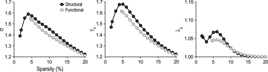
Topological properties of structural (dark‐grey circles) and functional (light‐grey circles) cortical networks. Small‐worldness (σ), clustering coefficient (γ _g), and path length (λ _g) of networks computed with positive partial correlations. Note that small‐worldness was slightly enhanced in structural when compared with functional cortical networks. This enhancement was due to the natural trend of structural connectivity networks to form segregated clusters (middle panel). The integration ability of functional networks was slightly higher than that in structural networks at lower sparsities, although the two networks behave randomly at higher sparsities (right panel).

Anatomical Location of Hubs and Modules in Structural and Functional Cortical Networks

Supporting Information Figures SM2 and SM3 show the topographic distribution of local and global hubs (based on node degree), respectively, supported by direct and indirect interactions for both structural and functional cortical networks. Cortical regions and Brodmann areas (BA) corresponding to hubs with a 100% probability across sparsities are listed in Supporting Information Tables SM1 (local hubs) and SM2 (global hubs). Further considerations about the anatomical location of both local and global hubs in structural and functional networks can be found in the Supporting Information (SM3).

Spatial overlapping of structural and functional hubs based on node degree is displayed in Figure 3. Table 1 includes BA corresponding to hubs with overlapping probability across sparsities above 40%. Most of the local hubs overlapping functional and structural networks were located in sensorimotor and unimodal association areas for both direct and indirect connections, whereas global hubs were mostly located over heteromodal association areas. Interestingly, most of these cortical regions corresponded to the classical resting‐state networks (see Supporting Information SM3 for further information on the anatomical location of global hubs in structural and functional cortical networks).

Figure 3.

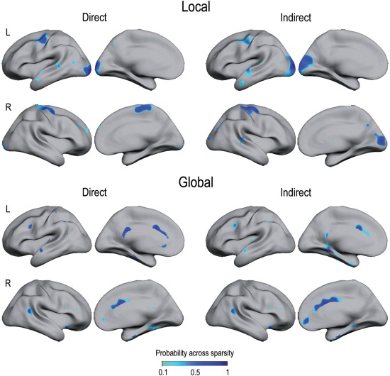
Overlapping of local and global hubs in structural and functional cortical networks. Overlapped hubs (based on node degree) were split into those with the highest number of direct connections (left column) and the highest number of indirect pathways (right column) in structural and functional networks, separately. The color scale represents the proportion of sparsities showing overlapped local/global hubs in both cortical networks. Note that overlapped local hubs were mostly allocated over unimodal association areas, whereas global hubs mainly appeared over heteromodal association areas. L = left; R = right.

Table 1.

Anatomical location of overlapped hubs in structural and functional cortical networks

Type of hub, cortical region	BA	Area	Probability across sparsities (%)
Local indirect
L Middle temporal gyrus	21	HA	90
R Superior parietal lobe	5	HA	75
R Inferior parietal lobe	40	HA	45
R Dorsolateral prefrontal cortex	9	HA	40
L/R Middle frontal gyrus	6, 8	UA	55–100
L/R Lingual gyrus	18	UA	90–100
L Inferior occipital gyrus	18	UA	55–90
L Middle occipital gyrus	18	UA	60
L/R Precentral gyrus	3, 4	SMA	40–100
R Calcarine sulcus	17	SMA	70
L Cuneus	17	SMA	65–90
L/R Lingual gyrus	17	SMA	50–85
Local indirect
R Precuneus	31	HA	85
L Superior temporal gyrus	22, 42	HA/UA	80
L/R Fusiform gyrus	18, 19	HA/UA	45–75
L Cuneus	18	UA	80–90
L Inferior temporal gyrus	20	UA	50
L Middle occipital gyrus	18	UA	95
L Superior occipital gyurs	18	UA	50
L/R Lingual gyrus	18	UA	40–70
R Inferior occipital gyrus	18	UA	60
R Middle frontal gyrus	6	UA	80
R Precentral gyrus	6	UA	60
L/R Cuneus	17	SMA	50–55
L/R Lingual gyrus	17	SMA	65–90
L/R Precentral gyrus	4	SMA	40–70
R Calcarine sulcus		SMA	100
R Poscentral gyrus	3	SMA	55
Global direct
L Inferior parietal lobe	40	HA	40–65
L/R Superior parietal lobe	7, 39	HA	55–80
R Cuneus	18	HA	60
R Dorsolateral prefrontal cortex	9	HA	90
R Parahippocampal gyrus	28	HA	45
R Posterior cingulate	31	HA	40
L/R Superior temporal gyrus	22	HA/UA	65–90
Global indirect
L Perirhinal cortex	36	HA	60
L/R Anterior cingulate	24, 32	HA	45–55
L/R Dorsolateral prefrontal cortex	9	HA	50–65
L/R Inferior parietal lobe	39, 40	HA	65–75
R Parahippocampal gyrus	38	HA	55
R Superior parietal lobe	7	HA	50
R Medial frontal gyrus	10	HA	45
R Ventrolateral prefrontal cortex	47	HA	40
L/R Superior temporal gyrus	22	HA/UA	70–90
L Fusiform gyrus	33	HA/UA	40
L Precentral gyrus	6	UA	65
R Cuneus	18	UA	65

BA: Brodmann areas; R: right; L: left; SMA: sensory‐motor area; UA: Unimodal association area; HA: heteromodal association area.

As the hierarchical clustering criterion used here to determine modularity does not consider the geometrical distance between nodes, no information can be drawn about the small‐worldness of modules integrated by local or global communities. To overcome this limitation, we estimated the degree of regional overlapping between these modules and local and global hubs (based on node degree) connected to other nodes through direct connections. Figure 4 shows module‐to‐hub coincidence across sparsities (above 40%) for the structural and functional network, separately. Cortical regions and BA corresponding to this overlapping are listed in Table 2 (structural network) and Table 3 (functional network). Results showed that the degree of overlapping between modules and hubs was higher for global than for local hubs in the two cortical networks. About half of the modules matched with global hubs, and 96% of the global direct hubs in the functional network (vs. 45% in the structural network) showed a modular structure. The degree of coincidence with local hubs decreased to 25%. Of all local hubs, 53.5% and 22.5% were modular in the structural and functional network, respectively. These ratios were similar when different sparsities were considered (above 60% and 100%, data not shown). Most of these modular hubs were restricted to heteromodal association areas; however, only those belonging to the functional network overlapped regions of different functional resting‐state networks involved in sensorimotor processing, executive functioning, memory and the default‐mode network (DMN; Fig. 4).

Figure 4.

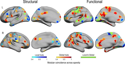
Regional distribution of cortical modules overlapping local (blue scale) and global hubs (red scale) in structural and functional networks. The color scale represents proportions for a modular node reached the hub criterion (node degree) across sparsities. Those modular nodes overlapping both local and global hubs are represented in green. L = left; R = right.

Table 2.

Anatomical location of modular nodes overlapping hubs in the structural network

Type of hub, cortical region	BA	Area	Probability across sparsities (%)
Local
L Inferior Frontal Gyrus	47	HA	90
L Medial Frontal Gyrus	10	HA	90
L Precuneus	7	HA	65–90
L Middle Temporal Gyrus	21, 39	HA	45–75
R Posterior Cingulate	29	HA	50
L Temporal Pole	38	HA/UA	40–100
L Inferior Occipital Gyrus	18	UA	80–100
L/R Cuneus	7, 17, 18, 19	UA	40–100
L Inferior Temporal Gyrus	20	UA	80
L Middle Occipital Gyrus	18, 19	UA	45–65
L Middle Frontal Gyrus	6, 9	SMA/HA	70–100
R Lingual Gyrus	17, 18	SMA/UA	55–100
R Postcentral Gyrus	2, 3	SMA	50–100
L Precentral Gyrus	4	SMA	95
Global
L Posterior Cingulate Gyrus	31	HA	55–95
L/R Inferior Frontal Gyrus	9, 47	HA	40–90
L/R Precuneus	7, 19, 31	HA	40–90
L Middle Temporal Gyrus	21, 39	HA	60–85
L Posterior Cingulate	30	HA	65
L Inferior Parietal Lobule	40	HA	60
L/R Anterior Cingulate Gyrus	24	HA	45–55
L Superior Parietal Lobule	7	HA	50
R Parahippocampal Gyrus	35	HA	50
L Superior Frontal Gyrus	8, 9	HA/UA	40–100
R Fusiform Gyrus	19, 37	HA/UA	95–100
R Medial Frontal Gyrus	6	HA/UA	100
L/R Superior Temporal Gyrus	13, 38, 39	HA/UA	45–90
L/R Inferior Temporal Gyrus	37	UA	45–90
R Cuneus	18	UA	60
R Middle Occipital Gyrus	19	UA	60
R Middle Frontal Gyrus	6, 10	SMA/HA	55–70
L Lingual Gyrus	18, 19	SMA/UA	45–95
L Precentral Gyrus	4	SMA	100
L/R Postcentral Gyrus	3, 43	SMA	40–45

BA: Brodmann areas; R: right; L: left; SMA: sensory‐motor area; UA: Unimodal association area; HA: heteromodal association area.

Table 3.

Anatomical location of modular nodes overlapping hubs in the functional network

Type of hub, cortical region	BA	Area	Probability across sparsities (%)
Local
L Middle Temporal Gyrus	21, 22, 37	HA	100
L Dorsal Anterior Cingulate	32	HA	80
L/R Fusiform Gyrus	18, 19, 20, 37	HA/UA	65–100
L/R Medial Frontal Gyrus	6, 10	HA/UA	65–100
L Inferior Occipital Gyrus	17, 18	UA	100
R Paracentral Lobule	6	UA	100
L Middle Occipital Gyrus	18	UA	80–90
L/R Cuneus	17, 18	UA	40–100
L Middle Frontal Gyrus	6, 9, 10	SMA/HA	40–100
L Superior Frontal Gyrus	6, 10	SMA/HA	70–100
L/R Lingual Gyrus	17, 18, 19	SMA/UA	40–100
L Precentral Gyrus	4, 6	SMA	65–100
L Postcentral Gyrus	2, 3	SMA	70–95
Global
L/R Middle Temporal Gyrus	21, 22, 37, 39	HA	100
R Inferior Frontal Gyrus	9	HA	100
R Uncus	38	HA	100
L/R Precuneus	7, 31, 39	HA	50–100
L Posterior Cingulate	30, 31	HA	90–100
L/R Parahippocampal Gyrus	19, 35	HA	95–100
L/R Inferior Parietal Lobule	40	HA	55–100
R Insula	13	HA	45–100
R Anterior Cingulate	24, 32	HA	40–100
L Superior Frontal Gyrus	9	HA	65
R Fusiform Gyrus	20, 37	HA/UA	100
L/R Middle Frontal Gyrus	6, 10	HA/UA	65–100
L/R Medial Frontal Gyrus	6, 10, 11	HA/UA	55–100
L/R Superior Temporal Gyrus	22, 41,13, 39	HA/UA	40–100
L Transverse Temporal Gyrus	41	UA	100
R Cuneus	18	UA	100
R Superior Parietal Lobule	7	UA	100
L/R Middle Occipital Gyrus	18, 37	UA	90–100
L Lingual Gyrus	18	UA	95
L/R Paracentral Lobule	5, 6	UA	45–100
L/R Precentral Gyrus	4, 6	SMA/UA	40–100
L/R Postcentral Gyrus	2, 3, 7	SMA	45–100

BA: Brodmann areas; R: right; L: left; SMA: sensory‐motor area; UA: Unimodal association area; HA: heteromodal association area; DMN: default‐mode network.

We further studied the pattern of connectivity of global modular hubs shared by structural and functional networks. Main results are illustrated in Supporting Information Figure SM4. This analysis confirmed the lack of frontoparietal and frontotemporal connections in the functional network, the reduced number of global modular hubs in the frontal lobe, and the fact that all nodes of the DMN were massively connected to each other.

Inferring F‐S Coupling From Topological Properties of Structural Cortical Networks

The strength of connectivity decreases with interregional distance in both structural and functional cortical networks [Lewis et al., 2009; Salvador et al., 2005]. Contrary to our expectation, the influence of within interregional distance on functional correlations was strongest for local direct cortical connections (Supporting Information Fig. SM5). To avoid this influence on network prediction, this factor was eliminated from subsequent analyses.

Figure 5 shows the influence of node attributes (all nodes, node degree, betweenness, and modularity) and type of connection (direct vs. indirect) on F‐S coupling for local (Fig. 5A) and global structural connections (Fig. 5B), after accounting for interregional distance (statistical thresholds are indicated by dashed lines). Regression analyses showed significant F‐S coupling (p < 0.05) for most types of connections and sparsities, except for those cortical regions supported by local indirect links. In the latter case, the degree of F‐S coupling only reached significance for sparsities above 10% when all nodes and node degree were considered. No significant differences were obtained for modularity. In the case of betweenness, F‐S coupling at the local level was only significant for direct connections and sparsities above 14%. Therefore, betweenness centrality was confirmed as the worst predictor of F‐S coupling in cortical networks supported by structural local connections.

Figure 5.

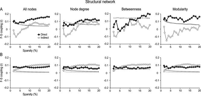
Functional‐structural (F‐S) coupling as a function of node attributes and intrinsic properties of structural network connections. F‐S coupling was displayed for direct (dark‐grey circles) and indirect connections (light‐grey circles) for cortical regions communicated through both local (A) and global interactions (B) across different levels of sparsity in the structural network. This analysis was performed for all nodes in the network, and for those nodes with either high centrality (based on node degree or betweenness) or high modularity. Dashed lines represent the statistical threshold (p <0.05) for each condition. Values above the dashed line represent significant F‐S correlations. Note that local direct structural connections were excellent predictors of F‐S coupling in cortical networks supported by local (A), but not by global elements (B).

Comparison among node attributes revealed that F‐S coupling supported by direct structural connections for both local and global interactions was strongest for modular nodes (p < 0.05, after correcting for multiple comparisons across sparsities). For indirect structural connections, F‐S coupling supported by centrality metrics and modularity was significantly higher for global connections compared to all nodes (p < 0.05, after correcting for multiple comparisons across sparsities). However, only local indirect connections for all nodes and node degree significantly accounted for the F‐S coupling, at least for sparsities above 10%.

When cortical networks were built with absolute values of both positive and negative partial correlations, levels of F‐S coupling increased for direct connections and decreased for indirect connections. Differences were more noticeable for global nodes (Supporting Information Fig. SM6). As in networks based on positive correlations, modular nodes connected through direct local connections in the structural network were the best predictors of F‐S coupling.

Inferring F‐S Coupling From Topological Properties of Functional Cortical Networks

We next investigated if F‐S coupling could be inferred from functional networks by using the above methodological approach. Figure 6 displays changes in F‐S coupling predicted by different types of functional connections. Comparison among node attributes showed that modularity was the best predictor of F‐S coupling between the two‐modality networks except for local indirect connections. In the latter case, the node degree showed the highest F‐S coupling level.

Figure 6.

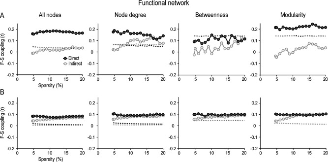
Functional‐structural (F‐S) coupling as a function of node attributes and intrinsic properties of functional network connections. F‐S coupling was displayed for direct (dark‐grey circles) and indirect connections (light‐grey circles) for cortical regions communicated through both local (A) and global interactions (B) across different levels of sparsity in the functional network. This analysis was performed for all nodes in the network, and for those nodes with either high centrality (based on node degree or betweenness) or high modularity. Dashed lines represent the statistical threshold (p <0.05) for each condition. Values above the dashed line represent significant F‐S correlations.

Apart from local betweenness, F‐S coupling reached significance for all conditions, except for functional nodes supported by local indirect connections, which resulted in a loss of F‐S coupling for sparsities below 10%. Although the degree of F‐S coupling was similarly predicted by structural or functional connections, this prediction was significantly enhanced by functional direct connections (p < 0.05 after correcting for multiple comparisons across sparsities). Thus, mean F‐S coupling for nodes with high modularity linked through direct connections was 26% higher in the functional than in the structural network at the local level, and 67% higher at global than at local level.

Levels of F‐S coupling increased when cortical networks were based on absolute values of positive and negative partial correlations. As illustrated in Supporting Information Figure SM7, modularity was corroborated as the best predictor of F‐S coupling for direct connections at both local and global levels. In contrast, F‐S coupling based on indirect connections never reached statistical significance.

DISCUSSION

Although evidence suggests that resting‐state functional connectivity is shaped by the structural organization of the brain [Greicius et al., 2009; Honey et al., 2009; Koch et al., 2002; Van den Heuvel et al., 2009], there is no histological validation of the anatomical substrate of resting‐state cerebral networks to date. This is congruent with previous evidence showing that DTI‐based structural connectivity patterns can hardly be inferred from resting‐state functional connectivity patterns based on hemodynamically‐driven changes derived from fMRI, suggesting that mechanisms underlying both types of connectivity may be unrelated [Honey et al., 2009]. Among novelties of the current study, we found that when structural and functional networks are exclusively based on measurements of cortical grey matter, like cortical thickness and glucose consumption, the F‐S coupling can be better inferred from functional than from structural network properties in normal aging. In this particular case, F‐S coupling is mainly constrained by properties supporting segregation of information (i.e., local direct connections and nodes with high modularity), at least when cortical networks are built on the only basis of positive correlations. If absolute correlation values are considered to create cortical networks, levels of F‐S coupling increase, especially for global connections. This finding should be interpreted cautiously not only because the nature of anti‐correlations is still under debate [e.g., Blumenfeld et al., 2004; Gong et al., 2012], but also because networks based on absolute correlations showed lower small‐world properties than those derived from networks only containing positive correlations (Fig. 2 and Supporting Information Fig. SM1). As will be argued below, findings derived from connectivity networks based on positive correlations correspond better to aging‐induced alterations in the functional integration of information.

Functional segregation is determined to a great extent by the network capacity for functional integration [Gong et al., 2012; Stam, 2010], suggesting that connectivity in local regions, mostly involved in specialized functions, depends on interactions among distant regions devoted to higher cognitive functions. This brain organization has demonstrated to maximize the efficiency of local and global information processing at relatively low cost in the human brain [Achard and Bullmore, 2007]. The balance between local and global network elements is affected by aging processes [Sun et al., 2012], which is consistent with structural neuroimaging evidence showing that aging‐related cognitive deficits not only arise from local cortical changes but also from failures in the integration of information between distant cortical regions [O'Sullivan et al., 2001].

Graph theory analyses applied to aging have revealed that both local and global efficiency are reduced in functional brain networks derived from resting‐state fMRI [Achard and Bullmore, 2007], these effects becoming more evident in frontal and parietal cortical regions. Accordingly, evidence suggests that the large fronto‐cingulo‐parietal module responsible for coordinating resting‐state brain circuits is segregated in anterior and posterior modules [Meunier et al., 2009], leading to increased intra‐modular connections in frontal and parietal regions in detrimental to inter‐modular connections [see also Chen et al., 2011]. This result is not restricted to resting state conditions, but also becomes evident during memory encoding and recognition [Wang et al., 2010]. Thus, increased path length in aging has been related to loss of frontoparietal connections [Wang et al., 2010], illustrating the impact of aging in the balance between integration and segregation, and confirming that a decrease in the capacity of integration of information is followed by an increase of segregation.

In line with these findings, we found less modular hubs within the frontal lobe and decreased connectivity between temporoparietal global modular hubs and frontal nodes in the functional network. The loss of frontal centrality and modularity was replaced by an enhancement of global modular hubs overlapping the primary somatosensory cortex (BA 2, 3), middle temporal gyrus (BA 39) and parahippocampal gyrus (BA 35) highly connected to other global modular hubs outside the frontal lobe (Supporting Information Fig. SM4). On the contrary, global modular nodes overlapping the DMN were highly connected to each other in the two networks. This increased connectivity was mainly evident within the posterior parietal lobe, particularly among regions like precuneus/posterior cingulate, angular gyrus, lingual gyrus, and inferior parietal lobe. This pattern of results, supported by anatomical evidence in monkeys [e.g., Cavada and Goldman‐Rakic, 1989], may indicate that the resting‐state network involved in the executive function is more affected by aging than other networks more related to somatosensory processing and memory function. This hypothesis has been extensively supported by studies suggesting that aging‐related cognitive deficits are primarily due to impaired executive control governed by the lateral prefrontal cortex [e.g., Braver and West 2008]. On the other hand, the pattern of connectivity specifically related to the DMN may be indicative of altered default‐mode activity. In this line, functional imaging studies performed in older adults have shown less deactivation in default‐mode regions, which could have important implications for information processing [Grady et al., 2006; Lustig et al., 2003; Miller et al., 2008].

Methodological Considerations

In the present study, local‐direct connections were defined as correlations between cortical regions whose centroids were separated by Euclidean distances below 30 mm. Several considerations should be taken into account regarding this criterion. On the one hand, the choice of 30 mm corresponds to the maximum length of short‐association fibers [Schüz and Braitenberg, 2002] but is also constrained by technical limitations. For instance, connections below 30 mm for cortical regions of 250 mm² would lead to a drastic decrease in the density of local connections. Thus, connections of 15 mm would lead to 53% of the cortical regions locally disconnected, whereas connections above 30 mm would result in highly similar networks at local and global levels [Sepulcre et al., 2010].

Furthermore, cortical distances below 30 mm do not necessarily reveal anatomical connections through short‐association fibers, mainly for two reasons. Firstly, because the Euclidean metric, although largely used in small‐world studies [Honey et al., 2009; Salvador et al., 2005; Sepulcre et al., 2010], neglects cortical geometry, and consequently, underestimates the length of connections between adjacent gyri, which is especially remarkable in the particular case of the corpus callosum and the arcuate fasciculum. The second reason is the controversy generated by comparing structural networks obtained with cortical thickness measurements and DTI‐based tractography. Although inter‐regional correlations of cortical thickness have shown similarities with respect to tractography maps [Lerch et al., 2006], other studies have found that only 35 to 40% of the positive thickness correlations match results from tractography [Gong et al., 2012]. Few human U‐fibers have been successfully detected with DTI tractography [Jian and Vemuri, 2007; Oishi et al., 2011], suggesting that DTI‐based graph theory analyses have no resolution enough to determine short‐association fibers.

CONCLUSIONS

Accumulating evidence suggests that coupling between structural and functional cortical connectivity discloses critical aspects of cortical organization in health [Greicius et al., 2009; Honey et al., 2009; Koch et al., 2002; Van den Heuvel et al., 2009] and disease [Skudlarski et al., 2010; Zhang et al., 2011]. However, node attributes and connection properties affecting this balance have remained unexplored. Here we show that the greatest level of F‐S coupling emerge in normal aging when inference is based on local direct connections of functional nodes with high modularity, meaning that F‐S coupling in aging is mainly constrained by those network elements involved in the segregation of information. Given that normal aging is associated with cognitive decline mainly affecting the frontal lobe and integration of information, the superior capacity of functional local network properties to predict F‐S may partially reveal these aging‐related deficits. Taken collectively, our results support the hypothesis that network coupling in aging strongly depends on node attributes and intrinsic properties of the functional network. Future research should unveil if impaired coupling between functional and structural cortical networks improve our ability to anticipate prevalent aging‐related neurodegenerative disorders.

Supporting information

Supporting Information

REFERENCES

- Achard S, Bullmore E (2007): Efficiency and cost of economical brain functional networks. PLoS Comput Biol 3:e17. [DOI] [PMC free article] [PubMed] [Google Scholar]
- Bassett DS, Bullmore E, Verchinski BA, Mattay VS, Weinberger DR, Meyer‐Lindenberg A (2008): Hierarchical organization of human cortical networks in health and schizophrenia. J Neurosci 28:9239–9248. [DOI] [PMC free article] [PubMed] [Google Scholar]
- Batouli AH, Boroomand A, Fakhri M, Sikaroodi H, Oghabian MA, Firouznia K (2009): The effect of aging on resting‐ state brain function: an fMRI study. Iran J Radiol 6:153–158. [Google Scholar]
- Bernhardt BC, Chen Z, He Y, Evans AC, Bernasconi N (2011): Graph‐theoretical analysis reveals disrupted small‐world organization of cortical thickness correlation networks in temporal lobe epilepsy. Cereb Cortex 21:2147–2157. [DOI] [PubMed] [Google Scholar]
- Blumenfeld H, McNally KA, Vanderhill SD, Paige AL, Chung R, Davis K, Norden AD, Stokking R, Studholme C, Novotny EJ Jr, Zubal IG, Spencer SS (2004): Positive and negative network correlations in temporal lobe epilepsy. Cereb Cortex 14:892–902. [DOI] [PubMed] [Google Scholar]
- Braver TS, West R (2008): Working memory, executive control and aging In: Craik FI, Salthouse TA, editors. The Handbook of Aging and Cognition, 3rd ed. New York: Psychology Press; pp 311–372. [Google Scholar]
- Cavada C, Goldman‐Rakic PS (1989): Posterior parietal cortex in rhesus monkey. II. Evidence for segregated corticocortical networks linking sensory and limbic areas with the frontal lobe. J Comp Neurol 287:422–445. [DOI] [PubMed] [Google Scholar]
- Chen ZJ, He Y, Rosa‐Neto P, Gong G, Evans AC (2011): Age‐related alterations in the modular organization of structural cortical network by using cortical thickness from MRI. Neuroimage 56:235–245. [DOI] [PubMed] [Google Scholar]
- Chen ZJ, He Y, Rosa P, Germann J, Evans AC (2008): Revealing modular architecture of human brain structural networks by using cortical thickness from MRI. Cereb Cortex 18:2374–2381. [DOI] [PMC free article] [PubMed] [Google Scholar]
- Cohen MX, Elger CE, Weber B (2008): Amygdala tractography predicts functional connectivity and learning during feedback‐guided decision‐making. Neuroimage 39:1396–1407. [DOI] [PubMed] [Google Scholar]
- Desikan RS, Segonne F, Fischl B, Quinn BT, Dickerson BC, Blacker D, Buckner RL, Dale AM, Maguire RP, Hyman BT, Albert MS, Killiany RJ (2006): An automated labeling system for subdividing the human cerebral cortex on MRI scans into gyral based regions of interest. Neuroimage 31:968–980. [DOI] [PubMed] [Google Scholar]
- Fan Y, Shi F, Smith JK, Lin W, Gilmore JH, Shen D (2011): Brain anatomical networks in early human brain development. Neuroimage 54:1862–1871. [DOI] [PMC free article] [PubMed] [Google Scholar]
- Ferrarini L, Veer IM, Baerends E, van Tol MJ, Renken RJ, van der Wee NJ, Veltman DJ, Aleman A, Zitman FG, Penninx BW, van Buchem MA, Reiber JH, Rombouts SA, Milles J (2009): Hierarchical functional modularity in the resting‐state human brain. Hum Brain Mapp 30:2220–2231. [DOI] [PMC free article] [PubMed] [Google Scholar]
- Fjell AM, Westlye LT, Amlien I, Espeseth T, Reinvang I, Raz N, Agartz I, Salat DH, Greve DN, Fischl B, Dale AM, Walhovd KB (2009): High consistency of regional cortical thinning in aging across multiple samples. Cereb Cortex 19:2001–2012. [DOI] [PMC free article] [PubMed] [Google Scholar]
- Freeman LC (1977): Set of measures of centrality based on betweenness. Sociometry 40:35–41. [Google Scholar]
- Gazzaley A, D'Esposito M (2007): Top‐down modulation and normal aging. Ann NY Acad Sci 1097:67–83. [DOI] [PubMed] [Google Scholar]
- Giovacchini G, Lerner A, Toczek MT, Fraser C, Ma K, DeMar JC, Herscovitch P, Eckelman WC, Rapoport SI, Carson RE (2004): Brain incorporation of 11C‐arachidonic acid, blood volume, and blood flow in healthy aging: a study with partial‐volume correction. J Nucl Med 45:1471–1479. [PubMed] [Google Scholar]
- Gong G, He Y, Chen ZJ, Evans AC (2012): Convergence and divergence of thickness correlations with diffusion connections across the human cerebral cortex. Neuroimage 59:1239–1248. [DOI] [PubMed] [Google Scholar]
- Grady CL, Springer MV, Hongwanishkul D, McIntosh AR, Winocur G (2006): Age‐related changes in brain activity across the adult lifespan. J Cogn Neurosci 18:227–241. [DOI] [PubMed] [Google Scholar]
- Greicius MD, Supekar K, Menon V, Dougherty RF (2009): Resting‐state functional connectivity reflects structural connectivity in the default mode network. Cereb Cortex 19:72–78. [DOI] [PMC free article] [PubMed] [Google Scholar]
- Hagmann P, Sporns O, Madan N, Cammoun L, Pienaar R, Wedeen VJ, Meuli R, Thiran JP, Grant PE (2010): White matter maturation reshapes structural connectivity in the late developing human brain. Proc Natl Acad Sci USA 107:19067–19072. [DOI] [PMC free article] [PubMed] [Google Scholar]
- Hänggi J, Wotruba D, Jäncke L (2011): Globally altered structural brain network topology in grapheme‐color synesthesia. J Neurosci 31:5816–5828. [DOI] [PMC free article] [PubMed] [Google Scholar]
- He Y, Dagher A, Chen Z, Charil A, Zijdenbos A, Worsley K, Evans A (2009): Impaired small‐world efficiency in structural cortical networks in multiple sclerosis associated with white matter lesion load. Brain 132:3366–3379. [DOI] [PMC free article] [PubMed] [Google Scholar]
- He Y, Chen Z, Evans A (2008): Structural insights into aberrant topological patterns of large‐scale cortical networks in Alzheimer's disease. J Neurosci 28:4756–4766. [DOI] [PMC free article] [PubMed] [Google Scholar]
- He Y, Chen ZJ, Evans AC (2007): Small‐world anatomical networks in the human brain revealed by cortical thickness from MRI. Cereb Cortex 17:2407–2419. [DOI] [PubMed] [Google Scholar]
- Honey CJ, Sporns O, Cammoun L, Gigandet X, Thiran JP, Meuli R, Hagmann P (2009): Predicting human resting‐state functional connectivity from structural connectivity. Proc Natl Acad Sci USA 106:2035–2040. [DOI] [PMC free article] [PubMed] [Google Scholar]
- Honey CJ, Kötter R, Breakspear M, Sporns O (2007): Network structure of cerebral cortex shapes functional connectivity on multiple time scales. Proc Natl Acad Sci USA 104:10240–10245. [DOI] [PMC free article] [PubMed] [Google Scholar]
- Jeon T, Mishra V, Uh J, Weiner M, Hatanpaa KJ, White CL III, Zhao YD, Lu H, Diaz‐Arrastia R, Huang H (2012): Regional changes of cortical mean diffusivities with aging after correction of partial volume effects. Neuroimage 62:1705–1716. [DOI] [PMC free article] [PubMed] [Google Scholar]
- Jian B, Vemuri BC (2007): A unified computational framework for deconvolution to reconstruct multiple fibers from diffusion weighted MRI. IEEE Trans Med Imaging 26:1464–1471. [DOI] [PMC free article] [PubMed] [Google Scholar]
- Koch MA, Norris DG, Hund‐Georgiadis M (2002): An investigation of functional and anatomical connectivity using magnetic resonance imaging. Neuroimage 16:241–250. [DOI] [PubMed] [Google Scholar]
- Langer N, Pedroni A, Gianotti LR, Hanggi J, Knoch D, Jäncke L (2012): Functional brain network efficiency predicts intelligence. Hum Brain Mapp 33:1393–1406. [DOI] [PMC free article] [PubMed] [Google Scholar]
- Lewis JD, Theilmann RJ, Sereno MI, Townsend J (2009): The relation between connection length and degree of connectivity in young adults: a DTI analysis. Cereb Cortex 19:554–562. [DOI] [PMC free article] [PubMed] [Google Scholar]
- Lerch JP, Worsley K, Shaw WP, Greenstein DK, Lenroot RK, Giedd J, Evans AC (2006): Mapping anatomical correlations across cerebral cortex (MACACC) using cortical thickness from MRI. Neuroimage 31:993–1003. [DOI] [PubMed] [Google Scholar]
- Lustig C, Snyder AZ, Bhakta M, O'Brien KC, McAvoy M, Raichle ME, Morris JC, Buckner RL (2003): Functional deactivations: change with age and dementia of the Alzheimer type. Proc Natl Acad Sci USA 100:14504–14509. [DOI] [PMC free article] [PubMed] [Google Scholar]
- Lv B, Li J, He H, Li M, Zhao M, Ai L, Yan F, Xian J, Wang Z (2010): Gender consistency and difference in healthy adults revealed by cortical thickness. Neuroimage 53:373–382. [DOI] [PubMed] [Google Scholar]
- Maris (2004): Randomization tests for ERP topographies and whole spatiotemporal data matrices. Psychophysiology 41:142–151. [DOI] [PubMed] [Google Scholar]
- Maslov S, Sneppen K (2002): Specificity and stability in topology of protein networks. Science 296:910–913. [DOI] [PubMed] [Google Scholar]
- McGinnis SM, Brickhouse M, Pascual B, Dickerson BC (2011): Age‐related changes in the thickness of cortical zones in humans. Brain Topogr 24:279–291. [DOI] [PMC free article] [PubMed] [Google Scholar]
- Meunier D, Achard S, Morcom A, Bullmore E (2009): Age‐related changes in modular organization of human brain functional networks. Neuroimage 44:715–723. [DOI] [PubMed] [Google Scholar]
- Miller SL, Celone K, DePeau K, Diamond E, Dickerson BC, Rentz D, Pihlajamaki M, Sperling RA (2008): Age‐related memory impairment associated with loss of parietal deactivation but preserved hippocampal activation. Proc Natl Acad Sci USA 105:2181–2186. [DOI] [PMC free article] [PubMed] [Google Scholar]
- Oishi K, Huang H, Yoshioka T, Ying SH, Zee DS, Zilles K, Amunts K, Woods R, Toga AW, Pike GB, Rosa‐Neto P, Evans AC, van Zijl PC, Mazziotta JC, Mori S (2011): Superficially located white matter structures commonly seen in the human and the macaque brain with diffusion tensor imaging. Brain Connect 1:37–47. [DOI] [PMC free article] [PubMed] [Google Scholar]
- Oishi K, Zilles K, Amunts K, Faria A, Jiang H, Li X, Akhter K, Hua K, Woods R, Toga AW, Pike GB, Rosa‐Neto P, Evans A, Zhang J, Huang H, Miller MI, van Zijl PC, Mazziotta J, Mori S (2008): Human brain white matter atlas: identification and assignment of common anatomical structures in superficial white matter. Neuroimage 43:447–457. [DOI] [PMC free article] [PubMed] [Google Scholar]
- Opgen‐Rhein R, Strimmer K (2007): Accurate ranking of differentially expressed genes by a distribution‐free shrinkage approach. Stat Appl Genet Mol Biol 6:9. [DOI] [PubMed] [Google Scholar]
- O'Sullivan M, Jones DK, Summers PE, Morris RG, Williams SC, Markus HS (2001): Evidence for cortical “disconnection” as a mechanism of age‐related cognitive decline. Neurology 57:632–638. [DOI] [PubMed] [Google Scholar]
- Peng J, Wang P, Zhou N, Zhu J (2009): Partial correlation estimation by joint sparse regression models. J Am Stat Assoc 104:735–746. [DOI] [PMC free article] [PubMed] [Google Scholar]
- Raz N, Lindenberger U, Rodrigue KM, Kennedy KM, Head D, Williamson A, Dahle C, Gerstorf D, Acker JD (2005): Regional brain changes in aging healthy adults: general trends, individual differences and modifiers. Cereb Cortex 15:1676–1689. [DOI] [PubMed] [Google Scholar]
- Romero‐Garcia R, Atienza M, Clemmensen LH, Cantero JL (2012): Effects of network resolution on topological properties of human neocortex. Neuroimage 59:3522–3532. [DOI] [PubMed] [Google Scholar]
- Salvador R, Suckling J, Coleman MR, Pickard JD, Menon D, Bullmore E (2005): Neurophysiological architecture of functional magnetic resonance images of human brain. Cereb Cortex 15:1332–1342. [DOI] [PubMed] [Google Scholar]
- Sanabria‐Diaz G, Melie‐Garcia L, Iturria‐Medina Y, Aleman‐Gomez Y, Hernandez‐Gonzalez G, Valdes‐Urrutia L, Galan L, Valdes‐Sosa P (2010): Surface area and cortical thickness descriptors reveal different attributes of the structural human brain networks. Neuroimage 50:1497–1510. [DOI] [PubMed] [Google Scholar]
- Schäfer J, Strimmer K (2005): A shrinkage approach to large‐scale covariance matrix estimation and implications for functional genomics. Stat Appl Genet Mol Biol 4:32. [DOI] [PubMed] [Google Scholar]
- Schüz A, Braitenberg V (2002): The human cortical white matter: quantitative aspects of cortico‐cortical long‐range connectivity In: Schüz A, Miller R, editors. Cortical Areas: Unity and Diversity. London: CRC Press; pp 377–385. [Google Scholar]
- Schwarz AJ, Gozzi A, Bifone A (2008): Community structure and modularity in networks of correlated brain activity. Magn Reson Imaging 26:914–920. [DOI] [PubMed] [Google Scholar]
- Sepulcre J, Liu H, Talukdar T, Martincorena I, Yeo BT, Buckner RL (2010): The organization of local and distant functional connectivity in the human brain. PLoS Comput Biol 10:e1000808. [DOI] [PMC free article] [PubMed] [Google Scholar]
- Skudlarski P, Jagannathan K, Anderson K, Stevens MC, Calhoun VD, Skudlarska BA, Pearlson G (2010): Brain connectivity is not only lower but different in schizophrenia: A combined anatomical and functional approach. Biol Psychiatry 68:61–69. [DOI] [PMC free article] [PubMed] [Google Scholar]
- Soffer SN, Vazquez A (2005): Network clustering coefficient without degree‐correlation biases. Phys Rev E Stat Nonlin Soft Matter Phys 71:057101. [DOI] [PubMed] [Google Scholar]
- Stam CJ (2010): Characterization of anatomical and functional connectivity in the brain: A complex networks perspective. Int J Psychophysiol 77:186–194. [DOI] [PubMed] [Google Scholar]
- Sun J, Tong S, Yang GY (2012): Reorganization of brain networks in aging and age‐related diseases. Aging Dis 3:181–193. [PMC free article] [PubMed] [Google Scholar]
- Supekar K, Uddin LQ, Prater K, Amin H, Greicius MD, Menon V (2010): Development of functional and structural connectivity within the default mode network in young children. Neuroimage 52:290–301. [DOI] [PMC free article] [PubMed] [Google Scholar]
- Tijms BM, Seriès P, Willshaw DJ, Lawrie SM (2012): Similarity‐based extraction of individual networks from gray matter MRI scans. Cereb Cortex 22:1530–1541. [DOI] [PubMed] [Google Scholar]
- Travers J, Milgram S (1969): An experimental study of the small world problem. Sociometry 32:425–443. [Google Scholar]
- Van den Heuvel MP, Mandl RC, Kahn RS, Hulshoff Pol HE (2009): Functionally linked resting‐state networks reflect the underlying structural connectivity architecture of the human brain. Hum Brain Mapp 30:3127–3141. [DOI] [PMC free article] [PubMed] [Google Scholar]
- Van den Heuvel MP, Mandl R, Luigjes J, Hulshoff, Pol H (2008): Microstructural organization of the cingulum tract and the level of default functional connectivity. J Neurosci 28:10844–10851. [DOI] [PMC free article] [PubMed] [Google Scholar]
- Van Wijk BC, Stam CJ, Daffertshofer A (2010): Comparing brain networks of different size and connectivity density using graph theory. PLoS One 5:e13701. [DOI] [PMC free article] [PubMed] [Google Scholar]
- Wang L, Li Y, Metzak P, He Y, Woodward TS (2010): Age‐related changes in topological patterns of large‐scale brain functional networks during memory encoding and recognition. Neuroimage 50:862–872. [DOI] [PubMed] [Google Scholar]
- Watts DJ, Strogatz SH (1998): Collective dynamics of “small‐world” networks. Nature 393:440–442. [DOI] [PubMed] [Google Scholar]
- Wu K, Taki Y, Sato K, Kinomura S, Goto R, Okada K, Kawashima R, He Y, Evans AC, Fukuda H (2012): Age‐related changes in topological organization of structural brain networks in healthy individuals. Hum Brain Mapp 33:552–568. [DOI] [PMC free article] [PubMed] [Google Scholar]
- Zhang Z, Liao W, Chen H, Mantini D, Ding JR, Xu Q, Wang Z, Yuan C, Chen G, Jiao Q, Lu G (2011): Altered functional‐structural coupling of large‐scale brain networks in idiopathic generalized epilepsy. Brain 134:2912–2928. [DOI] [PubMed] [Google Scholar]
Associated Data
This section collects any data citations, data availability statements, or supplementary materials included in this article.
Supplementary Materials