

Abstract
Using diffusion MRI, a number of studies have investigated the properties of whole‐brain white matter (WM) networks with differing network construction methods (node/edge definition). However, how the construction methods affect individual differences of WM networks and, particularly, if distinct methods can provide convergent or divergent patterns of individual differences remain largely unknown. Here, we applied 10 frequently used methods to construct whole‐brain WM networks in a healthy young adult population (57 subjects), which involves two node definitions (low‐resolution and high‐resolution) and five edge definitions (binary, FA weighted, fiber‐density weighted, length‐corrected fiber‐density weighted, and connectivity‐probability weighted). For these WM networks, individual differences were systematically analyzed in three network aspects: (1) a spatial pattern of WM connections, (2) a spatial pattern of nodal efficiency, and (3) network global and local efficiencies. Intriguingly, we found that some of the network construction methods converged in terms of individual difference patterns, but diverged with other methods. Furthermore, the convergence/divergence between methods differed among network properties that were adopted to assess individual differences. Particularly, high‐resolution WM networks with differing edge definitions showed convergent individual differences in the spatial pattern of both WM connections and nodal efficiency. For the network global and local efficiencies, low‐resolution and high‐resolution WM networks for most edge definitions consistently exhibited a highly convergent pattern in individual differences. Finally, the test–retest analysis revealed a decent temporal reproducibility for the patterns of between‐method convergence/divergence. Together, the results of the present study demonstrated a measure‐dependent effect of network construction methods on the individual difference of WM network properties. Hum Brain Mapp 36:1995–2013, 2015. © 2015 Wiley Periodicals, Inc.
Keywords: connectome, diffusion MRI, graph theory, test‐retest, inter‐subject variability, individual difference
INTRODUCTION
The human brain is a complex network with densely connected neural units in both structure and function [Sporns et al., 2005]. Advances in diffusion MRI techniques have made it possible to virtually reconstruct white matter (WM) tracts, which further allows the modeling of the human brain as a complex network/graph in vivo [Bullmore and Sporns, 2009; Le Bihan, 2003]. Graph theoretical approaches can then be applied to characterize topological architectures of whole‐brain WM networks [Rubinov and Sporns, 2010]. Using these techniques, a number of studies have revealed important topological properties for human brain WM networks, such as a small‐world organizational principle [Gong et al., 2009a; Iturria‐Medina et al., 2007], a set of highly connected hubs and highway connections [Gong et al., 2009a; Hagmann et al., 2008; Li et al., 2013], a modular structure [Hagmann et al., 2008; Hagmann et al., 2010; Yap et al., 2011], and a rich‐club attribute [van den Heuvel and Sporns, 2011; van den Heuvel et al., 2012, 2013].
Intriguingly, substantial individual differences (i.e., differences between individuals) have been observed in WM network properties, which may underlie intersubject variability in human cognitions and behaviors. For example, the topology of whole‐brain WM networks was shown to be significantly related to IQ scores and specific cognitive abilities across individuals [Li et al., 2009; Wen et al., 2011]. In addition, network variations can also be introduced by individual differences in age and sex [Gong et al., 2009b; Hagmann et al., 2010; Yan et al., 2011; Yap et al., 2011]. More importantly, specific topological properties of WM networks have shown significant changes in patients of brain diseases, such as stroke [Crofts et al., 2011], schizophrenia [van den Heuvel et al., 2010; Zalesky et al., 2011], Alzheimer's disease [Lo et al., 2010], multiple sclerosis [Shu et al., 2011], remitted geriatric depression [Bai et al., 2012], mild cognitive impairment [Shu et al., 2012], and attention deficit/hyperactivity disorder [Cao et al., 2013], which implies a potential role of the WM network topology as a biomarker for brain diseases [for a review, see Griffa et al., 2013].
While a number of studies have investigated WM networks using diffusion MRI, the construction method for WM networks differs substantially across studies. Specifically, the procedure of network construction usually involves two key issues: node and edge definition. For a WM network, nodes are typically defined as a gray matter (GM) area, and edges linking nodes are determined by diffusion MRI tractography. To date, a single choice for the node and edge definition remains elusive [Fornito et al., 2013]. For instance, the entire GM can be parcellated into either ∼100 (low‐resolution) or ∼1,000 units (high‐resolution), each of which represent a network node [de Reus and van den Heuvel, 2013]. Both deterministic and probabilistic tractography (PT) have been used to define edges, and multiple weighting strategies for edges have been proposed [Gong et al., 2009a, 2009b; Hagmann et al., 2008]. Given the differences in network construction methods, the results of WM networks become less comparable between studies, and some discrepant findings may be attributed to the methodological differences.
Recently, a few studies have exclusively assessed the effects of network construction methods (i.e., node/edge definition) on specific WM network properties (e.g., network efficiency, small‐worldness, and hub distribution), and substantial influences of the construction methods were observed [Bassett et al., 2011; Bastiani et al., 2012; Buchanan et al., 2014; Cammoun et al., 2012; Cheng et al., 2012a; Cheng et al., 2012b; Li et al., 2012; Zalesky et al., 2010]. However, these studies mainly focused on the method effects on the network properties for the same subjects. To date, how WM network construction methods affect individual differences of topological properties, and particularly if distinct construction methods can provide convergent or divergent patterns of individual difference, remains largely unknown. The individual differences in network properties are of great interests because these differences are the key issue in studying WM networks in a cross‐sectional manner, including group comparison, correlational analysis, and so forth. Therefore, a systematic evaluation of network construction methods in terms of individual differences is indispensable but still lacking. This evaluation can provide insightful implications for result interpretation across WM network studies.
In this study, we aim to exclusively assess the influence of different network construction methods on individual differences of WM network properties. Specifically, we sought to determine if different network construction methods would provide convergent or divergent individual differences. To address this issue, we applied 10 frequently used network construction methods across a healthy young adult population (57 subjects), and three aspects of WM networks were studied to assess individual differences: (1) a spatial pattern of WM connections, (2) a spatial pattern of nodal efficiency, and (3) network global efficiency and local efficiency.
MATERIALS AND METHODS
Participants
Data included in this study are a subset of the Connectivity‐based Brain Imaging Research Database (C‐BIRD) at Beijing Normal University (BNU). (http://fcon_1000.projects.nitrc.org/indi/CoRR/html/bnu_1.html). Fifty‐seven healthy young adults (female/male: 27/30; age: 23.19±2.13 years) were included in this study. Each subject was scanned twice with a 6‐week interval. All participants are right‐handed and have no history of neurological or psychiatric disorders. Written informed consent was obtained from each participant. The protocol was approved by the Institutional Review Board (IRB) of the State Key Laboratory of Cognitive Neuroscience and Learning at Beijing Normal University.
MRI Data Acquisition
All MRI scans were performed on a 3T Siemens Tim Trio MRI scanner at the Imaging Center for Brain Research, Beijing Normal University. The T1‐weighted images were acquired using a magnetization prepared rapid gradient echo sequence, and the imaging parameters were as follows: repetition time (TR) = 2,530 ms; echo time (TE) = 3.39 ms; inversion time = 1,100 ms; slice thickness = 1.33 mm; flip angle = 7°; no interslice gap; 144 sagittal slices covering the whole brain; matrix size = 256 × 256; field of view (FOV) = 256 × 256 mm2. For the diffusion‐weighted imaging (DWI) scans, a single‐shot twice‐refocused spin‐echo diffusion echo‐planar imaging (EPI) sequence was applied with the following parameters: TR = 8,000 ms; TE = 89 ms; 30 optimal diffusion‐weighted directions with a b‐value of 1,000 s/mm2 and one image with a b‐value of 0 s/mm2; data matrix = 128 × 128; FOV = 282× 282 mm2; slice thickness = 2.2 mm; 62 axial slices without interslice gap; voxel size = 2.2 × 2.2 × 2.2 mm3; number of average = 2.
WM Network Construction
Using a pipeline tool of diffusion MRI (i.e., PANDA) [Cui et al., 2013], we first preprocessed all DWI images using typical methods, for example, brain extraction, correction for eddy‐current distortion and simple head‐motion, correction for b‐matrix [Leemans and Jones, 2009], and computation for diffusion tensor and fractional anisotropy. The T1‐weighted image was segmented using the SPM8 package (http://www.fil.ion.ucl.ac.uk/spm/software/spm8/), yielding a WM mask in the T1 native space for each subject. The WM mask was further transformed into the diffusion native space for each subject, using the coregistration between the T1 and fractional anisotropy (FA) image. The resultant WM mask was applied as a constraint for subsequent tractography.
Two basic elements need to be determined for a whole‐brain network: nodes and edges. Here, 10 types of WM networks with distinct node/edge definitions were constructed for each subject. The construction flowchart is illustrated in Figure 1, using in‐house BrainNet Viewer package (http://www.nitrc.org/projects/bnv/) [Xia et al., 2013]. Defining details are described as follows.
Figure 1.
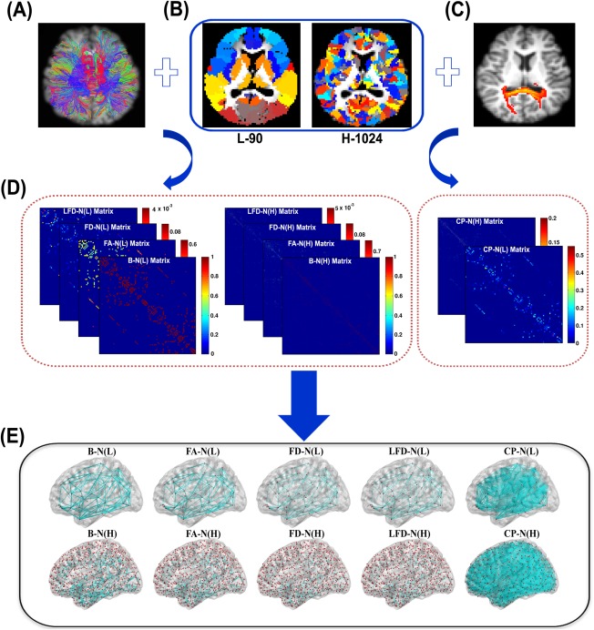
The schematic construction for the 10 WM networks in this study. (A) The outputs from the deterministic tractography. (B) The two gray matter parcellation schemes: L‐90 and H‐1024. Each patch with a specific color represents a node in WM networks. (C) The outputs from the probabilistic tractography. Both deterministic and probabilistic tractography were applied to infer connections between every two nodes within WM networks. (D) The example network matrices for the 10 construction methods. Eight networks are based on the deterministic tractography, and the other two are from the probabilistic tractography. (E) The 3D rendering for the 10 WM networks. B‐N, binary network; FA‐N, FA weighted network; FD‐N, fiber‐density weighted network; LFD‐N, length‐corrected fiber‐density network; CP‐N, connectivity‐probability weighted network. (L) and (H) denote networks at low‐resolution and high‐resolution, respectively. [Color figure can be viewed in the online issue, which is available at http://wileyonlinelibrary.com.]
Network Node Definitions
For a brain network at the macroscale, the entire GM was typically parcellated into a number of regions of interest (ROIs), each representing a network node. Here, we adopted two frequently used schemes: (1) AAL parcellation at low‐resolution (L‐90, in total 90 nodes/regions after excluding the cerebellum) [Tzourio‐Mazoyer et al., 2002]; (2) small‐ROI parcellation at high‐resolution (H‐1024, in total 1,024 nodes/ROIs after excluding the cerebellum). For the high‐resolution, the entire AAL template after excluding the cerebellum was parcellated uniformly into 1,024 small ROIs, using the algorithms developed by Zalesky et al. [2010]. The two parcellating atlases were originally defined in the standard Montreal Neurological Institute (MNI) space and were then transformed into the diffusion native space for each subject, as proposed previously [Gong et al., 2009a]. Briefly, the individual FA images were first coregistered to the T1‐weighted images. The T1‐weighted image was then nonlinearly normalized to the ICBM‐152 template in MNI space using FMRIB's Non‐linear Image Registration Tool (FNIRT, FSL, http://www.fmrib.ox.ac.uk/fsl/). Finally, the inverse transformations were applied to the two atlases (i.e., L‐90 and H‐1024 atlas) in the MNI space, resulting in native‐space GM parcelletions for each subject. The transforming procedures were also implemented by using PANDA.
Network Edge Definitions
Diffusion MRI tractography is required to determine if two GM nodes are anatomically connected. In previous WM network studies, both deterministic tractography (DT) and PT have been applied to infer between‐node connections [Gong et al., 2009a; Gong et al., 2009b; Hagmann et al., 2008]. Particularly, a WM network can be either binary or weighted, and diverse weighting strategies have been used for a weighted WM network [Meskaldji et al., 2013]. Using either DT or PT, we here adopted five weighting strategies to define edges within the WM networks, which have been frequently used in previous studies.
DT‐based edge definition
Here, DT was based on the fiber assignment continuous tracking algorithm with a tracking step size of 0.5 mm, which was applied to reconstruct whole‐brain tracts for each subject [Mori et al., 1999]. The tracking procedure was seeded from the center of each voxel within the WM mask, and was terminated if the turning angle was greater than 45° or the fiber entered a voxel out of the WM mask. All procedures were carried out using the Diffusion toolkit (http://trackvis.org) [Wang et al., 2007]. For each node pair, the linking fibers were then filtered out if the two terminal points are located in the two node regions, respectively. Based on the linking fibers between every two nodes, four types of edge weight were defined as follows.
Edge Definition 1: Binary network (B‐N). The weight only indicates the existence/absence of an edge between two nodes. Specifically, the edge weight was set to 1 if the fiber number was nonzero. Otherwise, it was set to 0 [Gong et al., 2009a].
Edge Definition 2: FA weighted network (FA‐N). The edge weight is defined as the mean FA values of voxels passed by the linking fibers [Li et al., 2009; Wen et al., 2011].
Edge Definition 3: Fiber‐Density weighted network (FD‐N). The edge weight is defined as the number of linking fibers after correcting for the nodal size , where and denote the number of voxels in regions i and j, respectively, and FN denotes the fiber number linking region i and region j [Cheng et al., 2012a]. The nodal size was corrected because a larger node/region is more likely to be touched by fibers in nature.
Edge Definition 4: Length‐corrected Fiber‐Density weighted network (LFD‐N). The weight is defined as the fiber density after additionally controlling for the fiber length , where denotes the average length of fibers linking region i and j [Hagmann et al., 2008; van den Heuvel and Sporns, 2011].
PT‐based edge definition
The PT was based on the algorithm proposed by Behrens et al. [2003, 2007], which has been implemented in FSL and used to construct WM networks [Gong et al., 2009b; Li et al., 2012]. Specifically, Markov Chain Monte Carlo sampling was used to estimate the parameters of the orientation distribution at each voxel with a Bayesian model with two‐fiber orientations [Behrens et al., 2003, 2007]. Each node region was selected as a seed region, and 5,000 fibers were sampled for each voxel within the region. For each sampled fiber, the tracking step size was set to be 0.5 mm. The edge weight based on the PT was defined as follows.
Edge Definition 5: Connectivity‐Probability weighted network (CP‐N). The connectivity probability from the seed region to the other target region was first computed as the number of fibers passing through the given target region divided by the total number of tracts sampled from the seed region. , where FN is the number of fibers passing through the target region j; n is the voxel number of the seed region i. Notably, the probability from i to j is not necessarily equivalent to the one from j to i because of the tractography dependence on the seeding location. The unidirectional edge weight was, therefore, defined as the average of these two probabilities [Cao et al., 2013; Gong et al., 2009b; Huang et al., 2013].
Taken together, two node definitions and five edge definitions were adopted in this study, which resulted in 10 separate WM networks for each subject. Each type of WM network can be represented by a symmetric matrix, in which each row and column represents a node and each element represents an edge as defined.
Network Thresholding
Due to data noise and algorithm errors, the raw individual networks are likely to contain spurious connections. Conceivably, a connection between two specific nodes is more likely to be reliable/real if it is consistently detected across individuals, and vice versa. We, therefore, controlled for spurious connections at the group level, as did previously [Gong et al., 2009a]. Specifically, for each node pair, a nonparametric sign‐test was applied by taking each individual as a sample, with the null hypothesis being that there is no existing connection (i.e., connectivity weight = 0). The Bonferroni method was used to correct for multiple comparisons across all node pairs within the network. For each type of WM networks, the node pair surviving a corrected P < 0.05 was deemed to have a connection. As a result, a binary matrix (1 for node pairs with a connection and 0 for node pairs without a connection) was generated for each type of WM networks. This binary mask was then applied to each individual network to remove the spurious connections for the subject.
For each type of WM networks, after above masking process, the density/sparsity of individual networks still differed. However, the between‐subject comparison in most network topological parameters typically requires the same network density [Fornito et al., 2013; van Wijk et al., 2010]. To control for this, we chose the minimum density/sparsity of networks across the 57 subjects. The individual network matrices with a higher density/sparsity were forced to reach the same density/sparsity by removing connections with the lowest edge weight. For each type of WM networks, the network density/sparsity became the same across subjects, improving between‐subject comparability of network measures below.
Network Measures
In graph theory, the measure of network efficiency was proposed to characterize the capacity of information communication within the network [Latora and Marchiori, 2001, 2003]. The related measures have a number of conceptual and technical advantages [Achard and Bullmore, 2007; Rubinov and Sporns, 2010], and are suitable to quantify complex networks with unconnected nodes that may exist in our obtained high‐resolution WM networks. We, therefore, chose these measures as the network measures of interest when assessing individual differences across network construction methods. Specifically, nodal efficiency, network global efficiency and local efficiency were calculated for each type of WM networks using in‐house Gretna package (http://www.nitrc.org/projects/gretna/).
Nodal Efficiency
Nodal efficiency (E nodal) is a measure that represents the capacity of a node to communicate with the other nodes of the network and is defined as follows:
| (1) |
where is the shortest path length between node i and node j, and N is the number of nodes of the network G.
Network Global Efficiency
Global efficiency is a global measure of the information transferring ability in the entire network, which is computed as the mean of nodal efficiency across all nodes of the network [Latora and Marchiori, 2001]:
| (2) |
where is the shortest path length between nodes i and j, and N is the number of nodes in the graph G.
Network Local Efficiency
Local efficiency corresponds to the efficiency of information flow within the local environment, which reflects the ability of a network to tolerate faults [Latora and Marchiori, 2001]. The local efficiency of a network is computed as follows:
| (3) |
where is the subgraph composed of the nearest neighbors of node i and the connections among them. Notably, the nearest neighbors for the were defined only in the context of graph/networks, without any spatial constrains in the brain.
Individual Differences of WM Network Properties
Specifically, individual differences of WM network properties were analyzed in three aspects: (1) the spatial pattern of WM connections, (2) the spatial pattern of nodal efficiency, and (3) the network efficiencies. For a specific WM network property, two construction methods were considered as convergent if they exhibited a similar pattern in individual differences; otherwise were considered as divergent.
Individual Differences in Spatial Pattern of WM Connections
The spatial pattern of WM connections reflects the edge distribution within the network, which represents the most basic information for the network connections. Here, the Pearson's correlation of edge weights was computed across all node pairs between every two subjects, which can reflect the degree of subject‐to‐subject similarity in the spatial pattern of WM connections [Bassett et al., 2011]. A high correlational value indicates a smaller difference in the spatial pattern between subjects. All subject‐to‐subject correlational values can be formulated as a symmetric matrix, in which each row and column represents a subject (in total 57), and element (i, j) is the correlational value between subject i and subject j. Particularly, the Pearson's phi correlation was applied between subjects for binary WM networks, which is applicable to binary cases (i.e., “1” or “0”) [Cremér, 1946]. Figure 2 illustrates the schematic diagram for estimating subject‐to‐subject similarity in the spatial pattern of WM connections. Together, ten subject‐to‐subject similarity matrices were generated, each for a WM network construction method.
Figure 2.

The schematic diagram for estimating subject‐to‐subject similarity in the spatial pattern of WM connections. (A) The WM networks of all subjects for a specific type of construction methods. The fiber‐density weighted networks at low‐resolution are displayed here as an example. (B) The WM connectivity matrix for all node pairs across all subjects. Each row and column represents a node pair and a subject, respectively. (C) The subject‐to‐subject matrix representing between‐subject similarity in the spatial pattern of WM connections. Each row and column represents a subject. The color represents Pearson correlation R‐values. (D) The scatter plot for the subject‐to‐subject Pearson correlation of connection weight. Here, the 40th and 50th subjects [marked out in (B) and (C)] were chosen as an example, and each circle represents a node pair. [Color figure can be viewed in the online issue, which is available at http://wileyonlinelibrary.com.]
For every pair of construction methods, the Pearson correlation of subject‐to‐subject similarity values was further applied across all subject pairs, which essentially captures the pattern similarity of the subject‐to‐subject matrix between methods. Therefore, a method‐to‐method similarity matrix was obtained, which reflected the degree of convergence of individual differences in the spatial pattern of WM connections.
Individual Differences in Spatial Pattern of Nodal Efficiency
The spatial pattern of nodal efficiency represents the nodal efficiency distribution within the network, which is essential to identify hub regions within the networks [Gong et al., 2009b; Hagmann et al., 2008]. Likewise, subject‐to‐subject similarity in the spatial pattern of nodal efficiency was estimated by the Pearson correlation across either 90 (low‐resolution) or 1,024 (high‐resolution) nodes within the network, which yielded another ten symmetric matrices (Fig. 3). Furthermore, by applying the Pearson correlation to the subject‐to‐subject similarity values across all subject pairs, a method‐to‐method similarity matrix was also generated, which represented the degree of convergence of individual differences in the spatial pattern of nodal efficiency.
Figure 3.

The schematic diagram for estimating subject‐to‐subject similarity in the spatial pattern of nodal efficiency. (A) The distribution of nodal efficiency of all subjects for a specific type of construction methods. Furthermore, the fiber‐density weighted networks at low‐resolution are displayed here. (B) The nodal efficiency matrix for all nodes across all subjects. Each row and column represents a node and a subject, respectively. (C) The subject‐to‐subject matrix representing between‐subject similarity in the spatial pattern of nodal efficiency. Each row and column represents a subject. The color represents Pearson correlation R‐values. (D) The scatter plot for the subject‐to‐subject Pearson correlation of connection weight. Again, the 40th and 50th subjects [marked out in (B) and (C)] were chosen as an example and each circle represents a node. [Color figure can be viewed in the online issue, which is available at http://wileyonlinelibrary.com.]
Individual Differences in Network Efficiencies
For network global and local efficiency, only one number is given to each network. Therefore, the subject‐to‐subject similarity could not be computed. The method‐to‐method similarity of the individual difference pattern was directly measured by computing the Pearson correlation of the efficiency values across all subjects. Here, a high correlational value indicates convergent individual differences of network efficiencies between methods. Likewise, we ended up with a method‐to‐method similarity matrix for network global and local efficiency.
Differences of Subject‐to‐Subject Similarity Across Methods
For the spatial pattern of both WM connections and nodal efficiency, we statistically compared subject‐to‐subject correlation values (i.e., R‐values) between the 10 construction methods. Notably, the degree of freedom for the R‐values differed between low‐resolution and high‐resolution networks. Therefore, we separately applied a one‐way repeated‐measure ANOVA at each resolution. Prior to statistical comparison, the R‐values were first converted to Z‐values using Fisher's r‐to‐z transformation.
Clustering Analysis of Network Construction Methods
To identify the convergence and divergence of individual difference pattern between network construction methods, we applied hierarchical clustering analysis to the four method‐to‐method similarity matrices. The results can be represented by a tree structure (referred to as a dendrogram), straightforwardly showing the clusters of construction methods at each hierarchical level. Here, the method‐to‐method similarity matrices were first converted to distance matrices (i.e., 1‐similarty matrix), representing the degree of difference between methods. The widely used average linkage agglomerative algorithm was then applied to each distance matrix, respectively [Legendre and Legendre, 1983]. Specifically, this bottom‐up clustering algorithm treated each construction method as a cluster at the beginning, and then merged the two clusters with the minimum distance into a new cluster. This procedure was iterated until only one cluster was reached. During each step, the distance between two clusters was defined as the average distance between members of the two clusters.
Test–Retest Reproducibility
We reran the above analyses with the second scans for all subjects and further assessed the cross‐session reproducibility for the patterns of individual differences as well as for the convergence of network construction methods. For each construction method, we first evaluated the reproducibility of the subject‐to‐subject similarity matrices for the spatial pattern of both WM connections and nodal efficiency. Specifically, for each method, we tested the Pearson correlation of all elements within the matrix between the two scans. Similarly, the reproducibility of the method‐to‐method similarity matrix for each WM network measure was tested by correlating all elements within the matrix between the two scans. In addition, we computed intraclass correlation coefficient (ICC) and coefficient of variation (CV) of the subject‐to‐subject similarities for the spatial pattern of both WM connections and nodal efficiency, and ICC and CV of the method‐to‐method similarities for each WM network measure [Bassett et al., 2011; Lachin, 2004]. Notably, there are multiple variants of ICC, and we used the version that was defined by a recent test‐retest study [Zuo et al., 2010]. Finally, the hierarchical clustering results were compared between the two sessions.
RESULTS
For each subject, we have built 10 different WM networks that involved two node definitions (i.e., L‐90 and H‐1024) and five edge definitions (i.e., binary, FA weighted, fiber‐density weighted, length‐corrected fiber‐density weighted, and connectivity‐probability weighted), as illustrated in Figure 1. These obtained WM networks exhibited very similar patterns with previously reported networks. The PT‐based networks had more connections compared with the DT‐based networks; and the high‐resolution networks showed a more sparsity than the low‐resolution ones.
Spatial Pattern of WM Connections
The subject‐to‐subject similarity matrix for each WM network was illustrated in Figure 4A, in which each element represents between‐subject similarity in the spatial pattern of WM connections. According to visual inspection, the four DT‐based low‐resolution networks consistently showed relatively high values compared with the high‐resolution networks. The one‐way repeated‐measure ANOVA revealed a significant method difference in subject‐to‐subject similarity values at both low‐resolution (P < 0.0001) and high‐resolution (P < 0.0001; Fig. 4B). In terms of the mean subject‐to‐subject similarity, the descending order is CP‐N > B‐N > FD‐N > LFD‐N > FA‐N for the low‐resolution networks and CP‐N > B‐N > FA‐N > LFD‐N >FD‐N for the high‐resolution networks. Notably, the CP‐N exhibited the highest mean subject‐to‐subject similarity at both low‐resolution and high‐resolution. Furthermore, the LSD post hoc test (i.e., the least significant difference test) found significant differences (P < 0.05) between every two adjacent networks in this order, except for FD‐N versus LFD‐N (P = 0.98) at low‐resolution.
Figure 4.
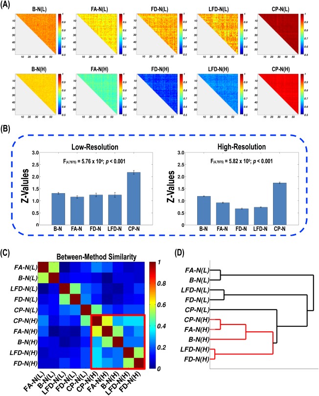
The method effects on individual differences in the spatial pattern of WM connections. (A) The 10 subject‐to‐subject similarity matrices for WM network construction methods. (B) The statistics of subject‐to‐subject similarity values for each method. The Pearson correlation R‐values were first converted to Z‐scores. According to the repeated‐measure ANOVA, significant differences were found across WM networks at low‐resolution and high‐resolution. (C) The similarity matrix representing method‐to‐method convergence of individual differences in the spatial pattern of WM connections. Each row and column represents a network construction method. The row and column were reordered to better visualize the clusters, which are marked by diagonal rectangles in red. (D) The hierarchical clustering dendrogram for construction methods. The lines are colored in terms of the clusters in (C). [Color figure can be viewed in the online issue, which is available at http://wileyonlinelibrary.com.]
The matrix of between‐method similarity was generated based on the subject‐to‐subject similarity. In total, 45 method pairs were examined, which can be further divided into three types: (1) within low‐resolution (10 in total, method‐to‐method similarity mean = 0.20, std = 0.19); (2) within high‐resolution (10 in total, mean = 0.35, std = 0.14); (3) between low‐resolution and high‐resolution (25 in total, mean = 0.16, std = 0.15). The between‐method similarity within high‐resolution was significantly higher than between low‐resolution and high‐resolution (t‐test, P = 0.0016) and showed a significant higher trend than within low‐resolution (P = 0.056). The within low‐resolution and between low‐resolution and high‐resolution types did not significantly differ (P = 0.63).
Hierarchical clustering was applied to identify convergence/divergence between the 10 construction methods. The row and column of the method‐to‐method similarity matrix was reordered for a better visualization of the clusters, and the hierarchical clustering dendrogram was illustrated (Fig. 4C,D). Clearly, the five high‐resolution WM networks can be grouped into a large cluster. Conceivably, the methods belonging to the same cluster have convergent individual difference patterns in the spatial pattern of WM connections. However, these methods are divergent with the methods outside of the cluster.
Spatial Pattern of Nodal Efficiency
Figure 5A illustrated the subject‐to‐subject matrices, which characterize the between‐subject similarity in the spatial pattern of nodal efficiency. Visual inspection also suggested relatively high similarity values for the four DT‐based low‐resolution networks compared with the high‐resolution networks. According to one‐way repeated‐measure ANOVA, the methods significantly differed at both low‐resolution (P < 0.0001) and high‐resolution (P < 0.0001; Fig. 5B). The descending order is B‐N > FA‐N > LFD‐N > CP‐N > FD‐N for the low‐resolution networks and CP‐N > B‐N > LFD‐N > FA‐N > FD‐N for the high‐resolution networks. The LSD test further revealed significant differences between every two adjacent networks in this order, except for FA‐N versus LFD‐N (P = 0.13) at low‐resolution.
Figure 5.
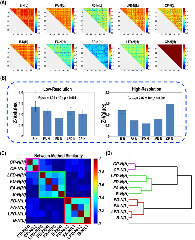
The method effects on individual differences in the spatial pattern of nodal efficiency. (A) The 10 subject‐to‐subject similarity matrices for WM network construction methods. (B) The statistics of subject‐to‐subject similarity values for each method. The Pearson correlation R‐values were first converted to Z‐scores. Significant differences were observed across WM networks at low‐resolution and high‐resolution. (C) The similarity matrix representing method‐to‐method convergence of individual differences in the spatial pattern of nodal efficiency. Each row and column represents a network construction method. The clusters are marked by diagonal rectangles in purple, red, and green. (D) The hierarchical clustering dendrogram for methods. The lines are colored in terms of the clusters in (C). [Color figure can be viewed in the online issue, which is available at http://wileyonlinelibrary.com.]
Using the subject‐to‐subject similarity of the spatial pattern of nodal efficiency, the between‐method similarity was also computed in a pairwise manner (within low‐resolution: mean = 0.26, std = 0.17; within high‐resolution: mean = 0.20, std = 0.14; between low‐resolution and high‐resolution: mean = 0.09, std = 0.16). Statistical comparisons indicated a significantly lower between‐method similarity of between low‐resolution and high‐resolution than within low‐resolution (P = 0.008), but no significant difference between within high‐resolution and both within low‐resolution (P = 0.40) and between low‐resolution and high‐resolution (P = 0.06).
The reordered method‐to‐method similarity matrix and the dendrogram from the hierarchical clustering of methods are demonstrated in Figure 5C,D. The matrix shows three obvious clusters. The first consisted of the four DT‐based high‐resolution networks, the second was formed by the four DT‐based networks at low‐resolution, and the other one was composed of the two PT‐based networks. At the highest level of the hierarchy, the 10 methods were largely divided into higher‐resolution and lower‐resolution, with the exception of the low‐resolution CP‐N being grouped into the high‐resolution family.
Network Global Efficiency and Local Efficiency
The individual values of network local and global efficiency were plotted for each WM network (Fig. 6). Expectedly, the exact values from different network construction methods differed significantly [Zalesky et al., 2010], but the subject courses of the values may exhibit a degree of similarity in shape, which suggested a convergent pattern of individual differences. The reordered matrix of between‐method similarity and the hierarchical clustering dendrogram are illustrated in Figure 6. Intriguingly, the low‐resolution and high‐resolution networks of FA‐N, LFD‐N and CP‐N were clustered together at the lowest level of the hierarchy, which suggested that individual differences in global and local efficiency were preserved across network resolutions.
Figure 6.
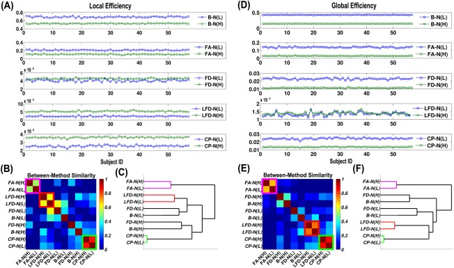
The method effects on individual differences in network global efficiency and local efficiency. (A) The subject course of local efficiency for the 10 WM networks. (B) The similarity matrix representing method‐to‐method convergence of individual differences in local efficiency. The obvious clusters are marked by diagonal rectangles in purple, red, and green. (C) The hierarchical clustering dendrogram for methods in terms of local efficiency. The lines are colored in purple, red, and green to match the clusters. (D) The subject course of global efficiency for the 10 WM networks. (E) The similarity matrix representing method‐to‐method convergence of individual differences in global efficiency. (F) The hierarchical clustering dendrogram for methods in terms of global efficiency. [Color figure can be viewed in the online issue, which is available at http://wileyonlinelibrary.com.]
Test–Retest Reproducibility
To assess the reproducibility, we tested correlations of the elements within each subject‐to‐subject similarity matrix or method‐to‐method similarity matrix between the two scans, respectively. For each WM network construction method, the subject‐to‐subject similarity in the spatial pattern of WM connections and nodal efficiency was significantly correlated (at least P < 0.001) between the two scans (Fig. 7), which indicated an acceptable reproducibility for the subject‐to‐subject similarity. As shown in Figure 8A, the four types of method‐to‐method similarity were also significantly correlated (at least P < 0.001).
Figure 7.

The test–retest reproducibility for subject‐to‐subject similarity values. (A) The results of two sessions for the spatial pattern of WM connections. (B) The results for the spatial pattern of nodal efficiency. In the scatter plots, the horizontal and vertical axes represent the first and second session, respectively. Each circle denotes a subject pair. [Color figure can be viewed in the online issue, which is available at http://wileyonlinelibrary.com.]
Figure 8.

The test–retest reproducibility for method‐to‐method similarity values and hierarchical clustering. (A) The method‐to‐method similarity matrices of two sessions for all network properties. For the scatter plots, the horizontal and vertical axes represent the first and second session, respectively. Each circle denotes a method pair. (B) The method dendrogram of two sessions for all network properties. The same network property was arranged in the same row for (A) and (B). [Color figure can be viewed in the online issue, which is available at http://wileyonlinelibrary.com.]
The ICC and CV values for the subject‐to‐subject similarity in the spatial pattern of WM connections and nodal efficiency were listed in Table 1. Specifically, the ICC values for the subject‐to‐subject similarity differed greatly across network types, with the CP‐N showing the highest values. In contrast, all network types consistently exhibited a low CV value for the subject‐to‐subject similarity (the spatial pattern of WM connections, mean = 1.6%, std = 0.94%; the spatial pattern of nodal efficiency, mean = 6.7%, std = 2.6%). For the between‐method similarity, the ICC and CV values were listed in Table 2. The ICC values were quite high for all network measures (mean = 0.91, std = 0.035), but the CV values differed greatly across network measures, with the spatial pattern of WM connection showing the lowest (CV = 27%) and the network global efficiency showing the highest (CV = 113.7%).
Table 1.
The ICC/CV for the subject‐to‐subject similarity of the spatial pattern
| WM connections | Nodal Efficiency | |||
|---|---|---|---|---|
| ICC | CV(%) | ICC | CV(%) | |
| B‐N(L) | 0.22 | 1.94 | 0.54 | 6.40 |
| B‐N(H) | 0.16 | 1.10 | 0.55 | 5.09 |
| FA‐N(L) | 0.57 | 2.02 | 0.59 | 4.59 |
| FA‐N(H) | 0.71 | 1.21 | 0.57 | 8.72 |
| FD‐N(L) | 0.63 | 2.30 | 0.65 | 10.59 |
| FD‐N(H) | 0.67 | 2.20 | 0.60 | 9.24 |
| LFD‐N(L) | 0.54 | 3.21 | 0.57 | 6.05 |
| LFD‐N(H) | 0.60 | 1.79 | 0.62 | 6.87 |
| CP‐N(L) | 0.78 | 0.27 | 0.68 | 7.75 |
| CP‐N(H) | 0.88 | 0.20 | 0.70 | 1.65 |
ICC, intraclass correlation coefficient; CV, coefficient of variation.
Table 2.
The ICC/CV for the method‐to‐method similarity
| ICC | CV(%) | |
|---|---|---|
| Spatial pattern of WM connections | 0.94 | 27.45 |
| Spatial pattern of nodal efficiency | 0.88 | 62.53 |
| Network local efficiency | 0.87 | 102.25 |
| Network global efficiency | 0.93 | 113.74 |
ICC, intraclass correlation coefficient; CV, coefficient of variation.
Finally, the clustering results from the second scan were highly consistent with the one from the first scan, irrespective of the type of method‐to‐method matrix (Fig. 8B).
DISCUSSION
By studying 10 different construction methods for WM networks, our present study demonstrated a substantial influence of the construction method on individual differences of specific WM network properties (e.g., the spatial pattern of WM connections, the spatial pattern of nodal efficiency, and network global efficiency and local efficiency). Our analysis revealed that a subset of network construction methods shared convergent patterns of individual differences, which contrasted other construction methods. More importantly, distinct network properties exhibited a convergent pattern of individual differences among specific sets of construction methods, which indicated that the method convergence depended on the network measures of interest.
To date, a number of studies have investigated individual differences (e.g., group comparison and correlational analysis) of human brain WM networks by using diffusion MRI, but with diverse network construction methods (i.e., node/edge definition) [Meskaldji et al., 2013]. For instance, network nodes have been defined at either low‐resolution (∼100 nodes) or high‐resolution (∼1,000 nodes), and network edges have been weighted differently such as binarization, FA, and fiber number. While a few studies have exclusively investigated method influences on specific network properties for the same subjects as well as their test–retest reproducibility [Bassett et al., 2011; Bastiani et al., 2012; Buchanan et al., 2014; Cheng et al., 2012a; Li et al., 2012; Zalesky et al., 2010], the method influences on individual differences remain largely unexplored. To our knowledge, this study was the first one to systematically assess method effects on individual differences, and therefore, may provide valuable implications for cross‐sectional WM network studies.
Effects of Node Definition on Individual Differences
For all WM networks, the subject‐to‐subject similarity values (i.e., R‐values) for the spatial pattern of WM connections and nodal efficiency were sufficiently high to reach the significance level (P < 0.05), which indicated a substantial similarity between subjects. Compatibly, the individual spatial patterns of nodal efficiency of WM networks have shown a high degree of similarity, which consistently suggests a structural core around medial posterior parietal areas across different subjects [Hagmann et al., 2008]. Our currently obtained WM networks also showed relatively high nodal efficiencies around medial posterior parietal regions, providing further support for this finding. Notably, the WM networks at low‐resolution exhibited higher subject‐to‐subject similarity values overall than the ones at high‐resolution in terms of the spatial pattern of either WM connections or nodal efficiency. This phenomenon is somewhat expected because the between‐subject variations are always more numerous at the finer scale, for example, high‐resolution networks. However, the lower subject‐to‐subject similarity values at high‐resolution than the low‐resolution might be related to the much higher degree of freedom when computing the Pearson correlation, which naturally leads to a lower correlational value.
Intriguingly, the method clustering analysis in terms of network global efficiency and local efficiency indicated that the low‐resolution and high‐resolution networks for most edge definitions were consistently grouped together, which suggested highly convergent patterns of individual differences for network efficiencies across network resolutions. This finding was supported by previous studies in which both low‐resolution and high‐resolution WM networks were analyzed. For example, the network global efficiency and clustering coefficient (corresponding to the network local efficiency) consistently showed a significant correlation with the developmental age for both low‐resolution and high‐resolution WM networks [Hagmann et al., 2010]. In addition, both low‐resolution and high‐resolution WM networks exhibited a significant group difference in the clustering coefficient between migraine patients and controls [Liu et al., 2013]. These results strongly supported a preservation of individual differences in network efficiencies across network resolutions.
Effects of Edge Definition on Individual Differences
In our current study, both DT and PT were applied to define network edges. Theoretically, the PT is advantageous because it has taken into account the uncertainty of fiber orientation estimation and fiber‐crossing issues [Bastiani et al., 2012; Behrens et al., 2007]. Strikingly, in terms of the spatial pattern of WM connections and nodal efficiency, PT‐based networks showed much higher subject‐to‐subject similarity than DT‐based networks, except for the spatial pattern of nodal efficiency at low‐resolution. This finding may relate to the large number of tracking sampling in PT, which likely lowers the between‐subject variations in presence/absence patterns of WM connections.
While the spatial pattern of WM connections and nodal efficiency at the same resolution showed convergent individual differences, the patterns of network global and local efficiency were largely divergent across edge definitions. In line with this, a few cross‐sectional studies investigating binary, FA‐weighted, or fiber‐density weighted WM networks in the same study have shown discrepant comparative or correlational results for either global efficiency or local efficiency between different weighted networks [Batalle et al., 2012; Li et al., 2009]. Also, discrepant results on network efficiency were observed between studies that investigated similar group comparisons. For example, Zalesky et al. [2011] found significant changes of efficiencies of binary networks (i.e., path length and clustering coefficient) in schizophrenia patients, as compared with controls. In contrast, another schizophrenia study reported no differences of network efficiencies between patients and controls, using FA‐weighted networks [van den Heuvel et al., 2010]. Given the divergent patterns of individual differences of network efficiency, some previously contradictory findings in group comparison or correlational analyses across studies may be attributed to the differences of edge definition.
Notably, the edge definition from DT was based on diffusion tensor model. While this model is very robust to noise and still represents the most widely used method in diffusion MRI applications, it has a limited capacity for resolving crossing fibers. This may result in the loss of some existing fibers and hence miss some connections (i.e., false negative) for our reconstructed WM networks. In addition, the inability to characterize crossing‐fiber situations has an impact on the tensor‐derived FA values (i.e., edge definition 2): the fiber‐crossing regions typically have very low FA values. This may separately influence the individual differences of the FA‐weighted network in our study, ultimately affecting the similarities between the FA‐weighted network and the other types of network. To address the fiber‐crossing issue, complex diffusion models can be estimated using more sophisticated methods such as constraint spherical deconvolution [Tournier et al., 2007; Tournier et al., 2004] and Q‐ball imaging [Tuch et al., 2003]. However, our current diffusion MRI acquisition does not allow for fitting these complex models. Future studies with more sophisticated diffusion models or diffusion imaging techniques, as well as finer imaging resolution or quality, are warranted to replicate our current findings.
Measure‐Specific Convergence/Divergence of Individual Differences Between Methods
The method clustering analysis provides a clue about the methods that exhibited convergent/divergent patterns of individual differences. Conceivably, the methods within the same cluster share convergent individual differences but less convergent or divergent individual differences with the methods outside of the cluster. Notably, the clustering results demonstrated that specific network construction methods may show convergent individual differences, but they strongly depend on network measures of interest, and distinct network properties may show convergent individual differences among different sets of methods. For example, the low‐resolution and high‐resolution networks for each edge definition were far from being grouped together according to the individual differences of the spatial pattern of either WM connections or nodal efficiency. However, the low‐resolution and high‐resolution networks for each edge definition were largely grouped together in terms of individual differences of network global efficiency and local efficiency, which suggested a convergent individual difference of global and local efficiency between low‐resolution and high‐resolution networks.
The measure‐specific convergence/divergence between methods has important implications for cross‐sectional WM network studies. For example, if one study focuses on the comparative or correlational analysis of network global efficiency and local efficiency across subjects or group, the statistical results are likely similar for WM networks at low‐resolution and high‐resolution, which implies less of a need for analyzing WM networks at multiple resolutions. However, if the study investigates the spatial pattern of nodal efficiency across subjects, conducting WM network analyses at multiple resolutions would be suggested because different network resolutions provide divergent subject contrast in the spatial patterns.
Reproducibility
The test–retest reproducibility of WM network properties has been recently evaluated, consistently suggesting an acceptable reproducibility for specific WM network measures (e.g., network global and local efficiency) [Bassett et al., 2011; Buchanan et al., 2014; Cheng et al., 2012a; Owen et al., 2013]. Notably, these studies mainly focused on reproducibility of network measures per se. In contrast, this study evaluated the reproducibility of the individual differences of specific network measures. For the first time, we confirmed that the subject‐to‐subject similarity of the spatial pattern of WM connections and nodal efficiency are temporally reproducible. More importantly, our analysis further demonstrated that the between‐method similarity of individual differences and method clusters were largely preserved across time, which indicated that convergence/divergence between network construction methods is temporally stable. The observed reproducibility of individual differences in WM network properties provides further supports for the decent reproducibility of the network properties per se [Bassett et al., 2011; Buchanan et al., 2014; Cheng et al., 2012a; Owen et al., 2013].
In line with previous studies showing differences on the test–retest reproducibility of network properties between network construction methods [Bassett et al., 2011; Buchanan et al., 2014], the degree of reproducibility of individual differences also depends on construction methods. Compatibly, a few recent studies have demonstrated the effects of tractography or related analyzing methods on the reproducibility of individual node–node connections [Lemkaddem et al., 2014; Smith et al., 2015], possibly serving as a potential source to the observed method‐dependent reproducibility for the whole‐brain network properties. Notably, the PT‐based networks overall exhibited a better test–retest reproducibility for the subject‐to‐subject similarity of the spatial pattern of WM connections and nodal efficiency. In addition, the PT using diffusion MRI has shown superior abilities to obtain accurate connections [Pestilli et al., 2014]. These compatible findings therefore provide support in favor of the PT for a wide range of applications in the future.
Limitations
A few issues need to be addressed. First, while this study has demonstrated method‐dependent individual differences for WM networks, we did not intend to provide a rule of thumb for the choice of network construction methods that should be largely based on specific question of interests. Given that differential biological underpinnings are linked to different network construction choices (particularly the edge weight definition), the presently observed differences of intersubject similarity or individual differences across different network construction methods are expected to some extent, possibly reflecting inherent different levels of inter‐subject variability across the differential biological underpinnings. For rigorous result comparisons across studies, identical network construction methods are therefore recommended. Second, since our diffusion MRI protocol did not include a field map acquisition, no preprocessing correction was made for EPI susceptibility distortion [Jones and Cercignani, 2010]. This may affect our findings to some extent, and therefore, needs to be addressed in the future. Third, technical details involved in WM network constructions can affect the network properties and their reproducibility. For example, tracking seeding strategies and termination criterion have shown an impact on the reproducibility of reconstructed tracts [Jones and Pierpaoli, 2005], as well as on the network topological parameters [Cheng et al., 2012b; Li et al., 2012]. Network thresholding for discarding spurious connections or configuring a customized network density/sparsity can also influence network properties [Cheng et al., 2012b; Fornito et al., 2013; Li et al., 2012]. In this study, we simply adopted one of the most common choices for these details. The effects of these detailed choices on the patterns of individual differences are beyond the scope of our current study and warrant separate studies in the future. Finally, we only assessed individual differences of WM network properties in a cohort of healthy subjects. Future studies are needed to explore the method influences on individual differences in disease. In addition, more investigations are warranted to examine the construction method influences on individual differences of other network measures such as the modular structure and rich‐club attributes [Hagmann et al., 2008; van den Heuvel and Sporns, 2011].
CONCLUSION
Our present study has demonstrated that network construction methods (e.g., spatial resolution for network nodes and weighting strategies for network edges) had a non‐negligible impact on the individual differences of WM networks. In particular, a subset of construction methods can provide convergent patterns of individual differences for specific network properties but are divergent with other construction methods. Importantly, the method convergence/divergence differed among network properties (e.g., spatial pattern of WM connections and nodal efficiency, and network global efficiency and local efficiency). These findings may provide valuable implications for understanding the intersubject variability of WM networks and comparing results across different studies.
ACKNOWLEDGMENTS
The authors sincerely thank Qixiang Lin for MRI data collection. The authors declare no competing financial interests.
REFERENCES
- Achard S, Bullmore E (2007): Efficiency and cost of economical brain functional networks. PLoS Comput Biol 3:e17. [DOI] [PMC free article] [PubMed] [Google Scholar]
- Bai F, Shu N, Yuan Y, Shi Y, Yu H, Wu D, Wang J, Xia M, He Y, Zhang Z (2012): Topologically convergent and divergent structural connectivity patterns between patients with remitted geriatric depression and amnestic mild cognitive impairment. J Neurosci 32:4307–4318. [DOI] [PMC free article] [PubMed] [Google Scholar]
- Bassett DS, Brown JA, Deshpande V, Carlson JM, Grafton ST (2011): Conserved and variable architecture of human white matter connectivity. Neuroimage 54:1262–1279. [DOI] [PubMed] [Google Scholar]
- Bastiani M, Shah NJ, Goebel R, Roebroeck A (2012): Human cortical connectome reconstruction from diffusion weighted MRI: The effect of tractography algorithm. Neuroimage 62:1732–1749. [DOI] [PubMed] [Google Scholar]
- Batalle D, Eixarch E, Figueras F, Munoz‐Moreno E, Bargallo N, Illa M, Acosta‐Rojas R, Amat‐Roldan I, Gratacos E (2012): Altered small‐world topology of structural brain networks in infants with intrauterine growth restriction and its association with later neurodevelopmental outcome. Neuroimage 60:1352–1366. [DOI] [PubMed] [Google Scholar]
- Behrens T, Woolrich M, Jenkinson M, Johansen‐Berg H, Nunes R, Clare S, Matthews P, Brady J, Smith S (2003): Characterization and propagation of uncertainty in diffusion–weighted MR imaging. Magnetic Reson Med 50:1077–1088. [DOI] [PubMed] [Google Scholar]
- Behrens T, Berg HJ, Jbabdi S, Rushworth M, Woolrich M (2007): Probabilistic diffusion tractography with multiple fibre orientations: What can we gain? NeuroImage 34:144–155. [DOI] [PMC free article] [PubMed] [Google Scholar]
- Buchanan CR, Pernet CR, Gorgolewski KJ, Storkey AJ, Bastin ME (2014): Test‐retest reliability of structural brain networks from diffusion MRI. Neuroimage 86:231–243. [DOI] [PubMed] [Google Scholar]
- Bullmore E, Sporns O (2009): Complex brain networks: Graph theoretical analysis of structural and functional systems. Nat Rev Neurosci 10:186–198. [DOI] [PubMed] [Google Scholar]
- Cammoun L, Gigandet X, Meskaldji D, Thiran JP, Sporns O, Do KQ, Maeder P, Meuli R, Hagmann P (2012): Mapping the human connectome at multiple scales with diffusion spectrum MRI. J Neurosci Methods 203:386–397. [DOI] [PubMed] [Google Scholar]
- Cao Q, Shu N, An L, Wang P, Sun L, Xia M‐R, Wang J‐H, Gong G‐L, Zang Y‐F, Wang Y‐F (2013): Probabilistic diffusion tractography and graph theory analysis reveal abnormal white matter structural connectivity networks in drug‐naive boys with attention deficit/hyperactivity disorder. J Neurosci 33:10676–10687. [DOI] [PMC free article] [PubMed] [Google Scholar]
- Cheng H, Wang Y, Sheng J, Kronenberger WG, Mathews VP, Hummer TA, Saykin AJ (2012a): Characteristics and variability of structural networks derived from diffusion tensor imaging. Neuroimage 61:1153–1164. [DOI] [PMC free article] [PubMed] [Google Scholar]
- Cheng H, Wang Y, Sheng J, Sporns O, Kronenberger WG, Mathews VP, Hummer TA, Saykin AJ (2012b): Optimization of seed density in DTI tractography for structural networks. J Neurosci Methods 203:264–272. [DOI] [PMC free article] [PubMed] [Google Scholar]
- Cremér H (1946): Mathematical Methods of Statistics. Princeton University Press, Princeton, NJ. [Google Scholar]
- Crofts JJ, Higham DJ, Bosnell R, Jbabdi S, Matthews PM, Behrens TE, Johansen‐Berg H (2011): Network analysis detects changes in the contralesional hemisphere following stroke. Neuroimage 54:161–169. [DOI] [PMC free article] [PubMed] [Google Scholar]
- Cui Z, Zhong S, Xu P, He Y, Gong G (2013): PANDA: A pipeline toolbox for analyzing brain diffusion images. Front Hum Neurosci 7:42. [DOI] [PMC free article] [PubMed] [Google Scholar]
- de Reus MA, van den Heuvel MP (2013): The parcellation‐based connectome: Limitations and extensions. Neuroimage 80:397–404. [DOI] [PubMed] [Google Scholar]
- Fornito A, Zalesky A, Breakspear M (2013): Graph analysis of the human connectome: Promise, progress, and pitfalls. Neuroimage 80:426–444. [DOI] [PubMed] [Google Scholar]
- Gong G, He Y, Concha L, Lebel C, Gross DW, Evans AC, Beaulieu C (2009a): Mapping anatomical connectivity patterns of human cerebral cortex using in vivo diffusion tensor imaging tractography. Cereb Cortex 19:524–536. [DOI] [PMC free article] [PubMed] [Google Scholar]
- Gong G, Rosa‐Neto P, Carbonell F, Chen ZJ, He Y, Evans AC (2009b): Age‐ and gender‐related differences in the cortical anatomical network. J Neurosci 29:15684–15693. [DOI] [PMC free article] [PubMed] [Google Scholar]
- Griffa A, Baumann PS, Thiran JP, Hagmann P (2013): Structural connectomics in brain diseases. Neuroimage 80:515–526. [DOI] [PubMed] [Google Scholar]
- Hagmann P, Cammoun L, Gigandet X, Meuli R, Honey CJ, Wedeen VJ, Sporns O (2008): Mapping the structural core of human cerebral cortex. PLoS Biol 6:e159. [DOI] [PMC free article] [PubMed] [Google Scholar]
- Hagmann P, Sporns O, Madan N, Cammoun L, Pienaar R, Wedeen VJ, Meuli R, Thiran JP, Grant PE (2010): White matter maturation reshapes structural connectivity in the late developing human brain. Proc Natl Acad Sci USA 107:19067–19072. [DOI] [PMC free article] [PubMed] [Google Scholar]
- Huang H, Shu N, Mishra V, Jeon T, Chalak L, Wang ZJ, Rollins N, Gong G, Cheng H, Peng Y and others. (2013): Development of human brain structural networks through infancy and childhood. Cereb Cortex. doi:http://10.1093/cercor/bht335. [DOI] [PMC free article] [PubMed] [Google Scholar]
- Iturria‐Medina Y, Canales‐Rodriguez EJ, Melie‐Garcia L, Valdes‐Hernandez PA, Martinez‐Montes E, Aleman‐Gomez Y, Sanchez‐Bornot JM (2007): Characterizing brain anatomical connections using diffusion weighted MRI and graph theory. Neuroimage 36:645–460. [DOI] [PubMed] [Google Scholar]
- Jones DK, Cercignani M (2010): Twenty‐five pitfalls in the analysis of diffusion MRI data. NMR Biomed 23:803–820. [DOI] [PubMed] [Google Scholar]
- Jones DK, Pierpaoli C (2005): Confidence mapping in diffusion tensor magnetic resonance imaging tractography using a bootstrap approach. Magn Reson Med 53:1143–1149. [DOI] [PubMed] [Google Scholar]
- Lachin JM (2004): The role of measurement reliability in clinical trials. Clin Trials 1:553–566. [DOI] [PubMed] [Google Scholar]
- Latora V, Marchiori M (2001): Efficient behavior of small‐world networks. Phys Rev Lett 87:198701. [DOI] [PubMed] [Google Scholar]
- Latora V, Marchiori M (2003): Economic small‐world behavior in weighted networks. Eur Phys J B 32:249–263. [Google Scholar]
- Le Bihan D (2003): Looking into the functional architecture of the brain with diffusion MRI. Nat Rev Neurosci 4:469–480. [DOI] [PubMed] [Google Scholar]
- Leemans A, Jones DK (2009): The B‐matrix must be rotated when correcting for subject motion in DTI data. Magn Reson Med 61:1336–1349. [DOI] [PubMed] [Google Scholar]
- Legendre P, Legendre L 1983. Numerical ecology. Elsevier Scientific Pub. Co, Amsterdam, The Netherlands. [Google Scholar]
- Lemkaddem A, Skiöldebrand D, Dal Palú A, Thiran JP, Daducci A (2014): Global tractography with embedded anatomical priors for quantitative connectivity analysis. Front Neurol 5:232. [DOI] [PMC free article] [PubMed] [Google Scholar]
- Li Y, Liu Y, Li J, Qin W, Li K, Yu C, Jiang T (2009): Brain anatomical network and intelligence. PLoS Comput Biol 5:e1000395. [DOI] [PMC free article] [PubMed] [Google Scholar]
- Li L, Rilling JK, Preuss TM, Glasser MF, Hu X (2012): The effects of connection reconstruction method on the interregional connectivity of brain networks via diffusion tractography. Hum Brain Mapp 33:1894–1913. [DOI] [PMC free article] [PubMed] [Google Scholar]
- Li L, Hu X, Preuss TM, Glasser MF, Damen FW, Qiu Y, Rilling J (2013): Mapping putative hubs in human, chimpanzee and rhesus macaque connectomes via diffusion tractography. Neuroimage 80:462–474. [DOI] [PMC free article] [PubMed] [Google Scholar]
- Liu J, Zhao L, Nan J, Li G, Xiong S, von Deneen KM, Gong Q, Liang F, Qin W, Tian J (2013): The trade‐off between wiring cost and network topology in white matter structural networks in health and migraine. Exp Neurol 248:196–204. [DOI] [PubMed] [Google Scholar]
- Lo CY, Wang PN, Chou KH, Wang J, He Y, Lin CP (2010): Diffusion tensor tractography reveals abnormal topological organization in structural cortical networks in Alzheimer's disease. J Neurosci 30:16876–16885. [DOI] [PMC free article] [PubMed] [Google Scholar]
- Meskaldji DE, Fischi‐Gomez E, Griffa A, Hagmann P, Morgenthaler S, Thiran JP (2013): Comparing connectomes across subjects and populations at different scales. Neuroimage 80:416–425. [DOI] [PubMed] [Google Scholar]
- Mori S, Crain BJ, Chacko V, Van Zijl P (1999): Three‐dimensional tracking of axonal projections in the brain by magnetic resonance imaging. Ann Neurol 45:265–269. [DOI] [PubMed] [Google Scholar]
- Owen JP, Ziv E, Bukshpun P, Pojman N, Wakahiro M, Berman JI, Roberts TP, Friedman EJ, Sherr EH, Mukherjee P (2013): Test‐retest reliability of computational network measurements derived from the structural connectome of the human brain. Brain Connect 3:160–176. [DOI] [PMC free article] [PubMed] [Google Scholar]
- Pestilli F, Yeatman JD, Rokem A, Kay KN, Wandell BA (2014): Evaluation and statistical inference for human connectomes. Nat Methods 11: 1058–1063. [DOI] [PMC free article] [PubMed] [Google Scholar]
- Rubinov M, Sporns O (2010): Complex network measures of brain connectivity: Uses and interpretations. Neuroimage 52:1059–1069. [DOI] [PubMed] [Google Scholar]
- Shu N, Liu Y, Li K, Duan Y, Wang J, Yu C, Dong H, Ye J, He Y (2011): Diffusion tensor tractography reveals disrupted topological efficiency in white matter structural networks in multiple sclerosis. Cereb Cortex 21:2565–2577. [DOI] [PubMed] [Google Scholar]
- Shu N, Liang Y, Li H, Zhang J, Li X, Wang L, He Y, Wang Y, Zhang Z (2012): Disrupted topological organization in white matter structural networks in amnestic mild cognitive impairment: Relationship to subtype. Radiology 265:518–527. [DOI] [PubMed] [Google Scholar]
- Smith RE, Tournier JD, Calamante F, Connelly A (2015): The effects of SIFT on the reproducibility and biological accuracy of the structural connectome. NeuroImage 104:253–265. [DOI] [PubMed] [Google Scholar]
- Sporns O, Tononi G, Kötter R (2005): The human connectome: A structural description of the human brain. PLoS Comput Biol 1:e42. [DOI] [PMC free article] [PubMed] [Google Scholar]
- Tournier JD, Calamante F, Gadian DG, Connelly A (2004): Direct estimation of the fiber orientation density function from diffusion‐weighted MRI data using spherical deconvolution. Neuroimage 23:1176–1185. [DOI] [PubMed] [Google Scholar]
- Tournier JD, Calamante F, Connelly A (2007): Robust determination of the fibre orientation distribution in diffusion MRI: Non‐negativity constrained super‐resolved spherical deconvolution. Neuroimage 35:1459–1472. [DOI] [PubMed] [Google Scholar]
- Tuch DS, Reese TG, Wiegell MR, Wedeen VJ (2003): Diffusion MRI of complex neural architecture. Neuron 40:885–895. [DOI] [PubMed] [Google Scholar]
- Tzourio‐Mazoyer N, Landeau B, Papathanassiou D, Crivello F, Etard O, Delcroix N, Mazoyer B, Joliot M (2002): Automated anatomical labeling of activations in SPM using a macroscopic anatomical parcellation of the MNI MRI single‐subject brain. NeuroImage 15:273–289. [DOI] [PubMed] [Google Scholar]
- van den Heuvel MP, Sporns O (2011): Rich‐club organization of the human connectome. J Neurosci 31:15775–15786. [DOI] [PMC free article] [PubMed] [Google Scholar]
- van den Heuvel MP, Mandl RC, Stam CJ, Kahn RS, Hulshoff Pol HE (2010): Aberrant frontal and temporal complex network structure in schizophrenia: A graph theoretical analysis. J Neurosci 30:15915–15926. [DOI] [PMC free article] [PubMed] [Google Scholar]
- van den Heuvel MP, Kahn RS, Goni J, Sporns O (2012): High‐cost, high‐capacity backbone for global brain communication. Proc Natl Acad Sci USA 109:11372–11377. [DOI] [PMC free article] [PubMed] [Google Scholar]
- van den Heuvel MP, Sporns O, Collin G, Scheewe T, Mandl RC, Cahn W, Goni J, Hulshoff Pol HE, Kahn RS (2013): Abnormal rich club organization and functional brain dynamics in schizophrenia. JAMA Psychiatry 70:783–792. [DOI] [PubMed] [Google Scholar]
- van Wijk BC, Stam CJ, Daffertshofer A (2010): Comparing brain networks of different size and connectivity density using graph theory. PLoS One 5:e13701. [DOI] [PMC free article] [PubMed] [Google Scholar]
- Wang R, Benner T, Sorensen A, Wedeen V (2007): Diffusion toolkit: A software package for diffusion imaging data processing and tractography. Proc Intl Soc Mag Reson Med 15:3720–3720. [Google Scholar]
- Wen W, Zhu W, He Y, Kochan NA, Reppermund S, Slavin MJ, Brodaty H, Crawford J, Xia A, Sachdev P (2011): Discrete neuroanatomical networks are associated with specific cognitive abilities in old age. J Neurosci 31:1204–1212. [DOI] [PMC free article] [PubMed] [Google Scholar]
- Xia M, Wang J, He Y (2013): BrainNet Viewer: A network visualization tool for human brain connectomics. PLoS One 8:e68910. [DOI] [PMC free article] [PubMed] [Google Scholar]
- Yan C, Gong G, Wang J, Wang D, Liu D, Zhu C, Chen ZJ, Evans A, Zang Y, He Y (2011): Sex‐ and brain size‐related small‐world structural cortical networks in young adults: A DTI tractography study. Cereb Cortex 21:449–458. [DOI] [PubMed] [Google Scholar]
- Yap PT, Fan Y, Chen Y, Gilmore JH, Lin W, Shen D (2011): Development trends of white matter connectivity in the first years of life. PLoS One 6:e24678. [DOI] [PMC free article] [PubMed] [Google Scholar]
- Zalesky A, Fornito A, Harding IH, Cocchi L, Yücel M, Pantelis C, Bullmore ET (2010): Whole‐brain anatomical networks: Does the choice of nodes matter? Neuroimage 50:970–983. [DOI] [PubMed] [Google Scholar]
- Zalesky A, Fornito A, Seal ML, Cocchi L, Westin CF, Bullmore ET, Egan GF, Pantelis C (2011): Disrupted axonal fiber connectivity in schizophrenia. Biol Psychiatry 69:80–89. [DOI] [PMC free article] [PubMed] [Google Scholar]
- Zuo XN, Kelly C, Adelstein JS, Klein DF, Castellanos FX, Milham MP (2010) Reliable intrinsic connectivity networks: Test‐retest evaluation using ICA and dual regression approach. Neuroimage 49:2163–2177. [DOI] [PMC free article] [PubMed] [Google Scholar]