

Abstract
The medial temporal lobe (MTL) plays a key role in learning, memory, spatial navigation, emotion, and social behavior. The improvement of noninvasive neuroimaging techniques, especially magnetic resonance imaging, has increased the knowledge about this region and its involvement in cognitive functions and behavior in healthy subjects and in patients with various neuropsychiatric and neurodegenerative disorders. However, cytoarchitectonic boundaries are not visible on magnetic resonance images (MRI), which makes it difficult to identify precisely the different parts of the MTL (hippocampus, amygdala, temporopolar, perirhinal, entorhinal, and posterior parahippocampal cortices) with imaging techniques, and thus to determine their involvement in normal and pathological functions. Our aim in this study was to define neuroanatomical landmarks visible on MRI, which can facilitate the examination of this region. We examined the boundaries of the MTL regions in 50 post‐mortem brains. In eight cases, we also obtained post‐mortem MRI on which the MTL boundaries were compared with histological examination before applying them to 26 in vivo MRI of healthy adults. We then defined the most relevant neuroanatomical landmarks that set the rostro‐caudal limits of the MTL structures, and we describe a protocol to identify each of these structures on coronal T1‐weighted MRI. This will help the structural and functional imaging investigations of the MTL in various neuropsychiatric and neurodegenerative disorders affecting this region. Hum Brain Mapp 35:248–256, 2014. © 2012 Wiley Periodicals, Inc.
Keywords: medial temporal lobe, anatomical landmarks, histological correlation, magnetic resonance images, memory
INTRODUCTION
The medial temporal lobe (MTL) is located at the ventromedial aspect of the temporal lobe. It is made up of several structures, namely the amygdaloid complex and the hippocampal formation, plus the parahippocampal region (temporopolar, perirhinal, and posterior parahippocampal cortices). Abundant evidence in the literature indicates that these MTL regions play a key role in different cognitive processes like memory [Squire et al., 2004; Suzuki and Amaral, 1994], spatial navigation [Epstein, 2005], emotion and social behavior [Aggleton, 2000; Amaral, 2003].
For a long time, the major way of examining the function of brain regions was invasive single‐cell recording and lesion studies. Using these techniques, it has been shown that each component of the MTL makes different contribution to cognitive functions. For instance, the perirhinal cortex was found to be critically involved in visual processing, especially in visual recognition memory [Malkowa et al., 2001; Meunier et al., 1993; Rauchs et al., 2006] whereas entorhinal and posterior parahippocampal cortices, and hippocampus play a major role in processing spatial information, each of these regions being implicated in distinct aspects of spatial memory and spatial navigation [Alvarado and Bachevalier, 2005; Eichenbaum et al., 1999; Ekstrom et al., 2003; Malkova and Mishkin, 2003; Moser and Moser, 2008; O'Keefe and Dostrovsky, 1971; Suzuki et al., 1997]. The temporopolar cortex has been involved in semantic memory [Hodges et al., 1992; Kapur et al., 1992], and the amygdala in fear conditioning [Ohman and Mineka, 2001], motivation [Rolls, 1992], social behavior [Adolphs 2010; Amaral, 2003; Meunier and Bechevalier, 2002], and in a wide variety of tasks with an emotional component [Aggleton, 1992; Aggleton, 2000; Gallagher and Chiba, 1996]. Single‐cell recording and lesion studies also demonstrated the different involvement of each MTL structure in relational and context‐dependent memory [Gallagher and Chiba, 1996; Squire, 1992; Suzuki and Eichenbaum, 2000].
The improvement of imaging techniques in the last decades opened a new way in the examination of these regions. Functional magnetic resonance imaging (fMRI) and positron emission tomography (PET) studies confirmed and further specified the above findings [Adolphs, 2010; Binder et al., 2009; Blaizot et al., 2000; Davachi and Wagner, 2002; Davachi, 2006; Epstein, 2005; Pessoa, 2010; Rauchs et al., 2006; Squire et al., 2004]. Among these neuroimaging techniques, magnetic resonance imaging allows the examination of the in vivo brain anatomy, and its changes as a result of diseases. This noninvasive technique has revealed hippocampal atrophy not only in various dementias [Laakso et al., 1996] but also in schizophrenia, major depression, and obsessive‐compulsive disorders [Geuze et al., 2005; Schumann et al., 2004]. Amygdala atrophy has been reported in children with autism [Schumann et al., 2004], whereas temporopolar atrophy has been described in semantic dementia [Hodges et al., 1992]. The entorhinal, perirhinal, and posterior parahippocampal cortices are severely affected in patients with Alzheimer's disease [Braak and Braak, 1991; Juottonen et al., 1998; Thangavel et al., 2008] and the neuropathological changes found there might explain most of the regional hypometabolism and memory deficits of these patients [Blaizot et al., 2002; Meguro et al., 1999]. However, since cytoarchitectonic boundaries are not visible on magnetic resonance images (MRI), it is difficult to identify precisely the different MTL cortices (temporopolar, entorhinal, perirhinal, and posterior parahippocampal cortices) using this technique.
Different methods are used to locate the MTL regions on MRI. The most common one is to compare the MRI to anatomical atlases. The atlas by Duvernoy [Duvernoy, 1988] is one of the most frequently used [Bartzokis et al., 1998; Bernasconi et al., 2003; von Gunten and Ron, 2004; Watson et al., 1992]. It shows clear delineation of the different MTL regions, but it is based on a single brain. Therefore, the high inter‐individual neuroanatomical variability makes difficult the direct application of the atlas boundaries to the actual MRI slices. A more robust method is the use of probabilistic atlases [Amunts et al., 2005]. However, this atlas was generated from only 10 post‐mortem brains. Moreover, most of the existing segmentation protocols were designed for one or few MTL structures [Insausti et al., 1998a], and combining different protocols can result in overlap of the neighbouring regions.
Here we present an account of anatomical landmarks for rostro‐caudal segmentation of the MTL on MRI. These landmarks were defined on post‐mortem MRI after identifying the cytoarchitectonic fields and their boundaries on neuroanatomical series. The protocol we propose corroborates and extends that previously developed for the temporopolar, perirhinal, and entorhinal cortices by Insausti et al. 1998a. We extended it to the amygdala, hippocampus and the posterior parahippocampal cortex to complete the set of MTL structures relevant to memory function and neuropsychiatric diseases. The present protocol allows the identification of all these MTL regions following a rostro‐caudal sequence of anatomical landmarks identifiable on structural MRI, without the need of high‐resolution sequences and/or time‐consuming image analysis.
METHODS AND MATERIALS
The boundaries of the MTL regions were defined on histological sections of 50 post‐mortem brains. Post‐mortem MRI were then examined for clear and reliably identifiable gross anatomical landmarks such as the limen insulae that could be easily related to cytoarchitectonic boundaries. If a boundary did not correspond to any anatomical landmark visible on MRI, the most reliable landmark allowing the best location of the boundary was selected, and the average distance between the landmark and the boundary on the histological series was computed. These gross anatomical landmarks and their averaged distances from the histological boundaries were then verified on eight brains with both post‐mortem MRI and histological preparations. These landmarks were later applied to an independent set of in vivo MRI from 26 healthy elderly people.
SUBJECTS
Fifty post‐mortem brains (mean age: 55.6 ± 24 years) were examined for cytoarchitectonic boundaries among the different regions in the MTL. Histological analyses of the brains were performed according to the protocol of the Human Neuroanatomy Laboratory in Albacete (Spain) as reported previously [Insausti et al., 1998a]. In eight cases (mean age: 54 years; five men), a post‐mortem MRI was also obtained (MRI/histology series).
In vivo MRI of 26 healthy volunteers (13 men; age: 73.6 ± 8.4 years, range: 53–88 years) were also acquired. All subjects were cognitively normal as assessed by the Mattis Dementia rating scale (mean score: 137.4 ± 4.4), had at least 5 years of education and a modified Hachinski score less than or equal to two. Those with medical history of neurological or psychiatric disease, alcoholism, depression or use of medication affecting the central nervous system were excluded from the study. All subjects gave their written informed consent prior to the experiment that was approved by the Lower Normandy Ethics committee (Consultative Committee for the Protection of Persons taking part in Biomedical Research).
MRI ACQUISITION
In each of the eight post‐mortem cases, coronal MRI were obtained in a 3T scanner (Siemens, Erlangen, Germany) using a head matrix coil and sequence First T1‐SE: repetition time (TR): 500 ms; echo time (TE): 10 ms; matrix 576 × 576; field of view (FOV): 250 mm; 94 slices; slice thickness 1 mm; resolution: 0.43 × 0.43 × 1 mm3; acquisition time: 59 min. The brains were processed afterwards as reported previously [Insausti et al., 1998a].
The in vivo MRI were acquired on a GE Genesis‐Signa (General Electric Medical Systems, USA) 1.5T system using T1‐weighted 3D inversion recovery sequence (TR = 11.2 ms, TE = 32.6 ms, TI = 600 ms, flip angle = 10°, FOV = 240 mm, image matrix = 256 × 256, 124 coronal slices, 1.5 mm slice thickness, resolution: 0.94 × 0.94 × 1.5 mm3). For image analysis, we used the MIPAV software (Center for Information Technology, NIH, USA). Before segmentation, the coronal images were aligned to be perpendicular to the anterior–posterior commissural line and resampled to 0.5 × 0.5 × 1.5 mm3 resolution using linear interpolation.
RESULTS
Rostro‐Caudal Limits of the MTL Structures
The MTL is made up of the amygdaloid complex, the hippocampal formation, and the parahippocampal region (temporopolar, perirhinal, and posterior parahippocampal cortices, all of which present strong connections with the entorhinal cortex). Under the term amygdaloid complex (amygdala for brevity), we include both the olfactory part (cortical amygdala and adjacent pyriform cortex) and the baso‐lateral complex of the amygdala. The hippocampal formation comprises the hippocampus (dentate gyrus, hippocampus proper [CA1‐CA3 fields] and subiculum), presubiculum, parasubiculum, and the entorhinal cortex.
The segmentation, performed on coronal MRI with the help of multiplanar views, requires the identification of a series of gross anatomical landmarks which relate to distinct cytoarchitectonic MTL fields, namely the collateral sulcus (CS), the limen insulae (LI), the rostral and caudal limits of the hippocampus, the hippocampal‐amygdaloid transitional area (HATA), the gyrus intralimbicus (GIL) and the posterior crus of the fornix. Using these seven landmarks, the boundaries of the MTL structures can be determined with accuracy by following a rostro‐caudal sequence (Figs. 1 and 2):
The temporopolar cortex appears at the most rostral tip of the temporal lobe (Fig. 3A,B). It extends for about 15 mm posteriorly and is replaced by the perirhinal cortex, the beginning of which is related to the appearance of the CS. The rostral limit of the CS usually appears slightly rostral to the LI (Fig. 4) but individual variability can be high [Ding and Van Hoesen, 2010; Insausti et al., 1995, 1998a]. The CS can be best identified slightly caudal to its anterior extreme, where the five temporal gyri (superior, middle and inferior temporal gyri, fusiform gyrus, and parahippocampal gyrus) become visible (Fig. 5D); from this point, the CS can be followed anteriorly up to its beginning. The rostralmost CS was defined on the slice where both the indentation of the grey matter and the bifurcation of the white matter were visible on the ventro‐medial part of the anterior temporal lobe (Fig. 1C). This very first slice with a small indentation on the pial surface is more difficult to detect on MRI than on histological sections due to the lower resolution of the MRI. Consequently, the CS can appear more posterior on in vivo MRI than on histological sections. The similar variability in the distance between the temporal pole and CS on MRI and histological series (SD of the mean distance: 3.4 and 3.7, respectively), however, suggests that the high variability in locating the CS results from anatomical difference among subjects and not from the technique.
The LI, which is the point where the frontal lobe becomes continuous with the temporal lobe, orients the beginning of both the amygdala and the entorhinal cortex [Insausti et al., 1998a], and in some cases the beginning of the perirhinal cortex. Based on the cytoarchitectonic examination, the perirhinal cortex begins about 1.5 mm anterior to the LI if the CS starts at the level of or posterior to LI. The amygdala starts at the level of LI, and 2 mm on average further caudally the entorhinal cortex begins [Insausti and Amaral, 2004], medial to the perirhinal cortex.
The rostralmost portion of the hippocampus (i.e., the subiculum) can be detected just prior or in the rostralmost extreme of the lateral ventricle, usually as an ovoid mass located in the rostral tip of the lateral ventricular cavity, under the amygdala. This is considered as the first section of the hippocampus proper.
The HATA indicates the most caudal part of the amygdala [Pitkanen, 2002], and it starts about 4 mm behind the beginning of the hippocampus. Although the amygdala can extend further posteriorly, it is difficult to visualize it on MRI and it would represent only a very small additional volume. Besides, using this definition, one avoids confusion of the tail of the caudate nucleus with the very posterior amygdaloid nuclei. HATA is approximately coincident with the commencement of the choroidal fissure; this landmark can be identified on the last slice where the uncus is continuous with the base of the brain.
The caudal limit of the entorhinal cortex lies about 1.5 mm behind the last slice where the GIL is present as a small round structure medial to the usual profile of the hippocampus (Fig. 5A–C). This point is also considered as the end of the hippocampal head. Shortly after this point (3 mm on average), the caudal limit of the perirhinal cortex can be established.
The perirhinal cortex is replaced caudally by the posterior parahippocampal cortex, which extends as far back as the anterior limit of the parieto‐occipital fissure (or anterior calcarine fissure) [Insausti et al., 1998b]. The size of this sulcus can be quite small at its anterior end, and therefore, very difficult to assess on MRI. But we found that the anterior end of the calcarine sulcus was very close to the level when the fimbria turns upwards to continue as the posterior pillars of the fornix under the corpus callosum. This unmistakable landmark, named the posterior crus of the fornix, is located only 4 mm anterior to the rostralmost part of the calcarine fissure [Insausti and Amaral, 2004], and it is always present and readily visible on MRI. Because the end of the posterior parahippocampal cortex tapers off, the last 2–3 mm account for a small portion of the total volume of this MTL region. Therefore, the caudal limit of the posterior parahippocampal cortex can be accurately defined as 1.5 mm posterior to the crus of the fornix.
The hippocampus ends right after this point as a mass of ovoid grey matter medial to the lateral ventricle. Underneath the end of the hippocampus lies the region occupied by the retrosplenial cortex, at the isthmus of the parahippocampal gyrus.
Figure 1.
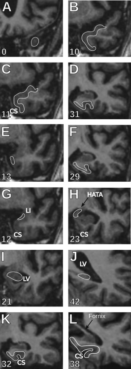
Rostro‐caudal limits of the MTL regions. (A,B) Temporopolar cortex: The most anterior slice containing the temporopolar cortex is where the grey matter of the temporal cortex is first visible in the middle cranial fossa (A). The sagittal views (Fig. 3A,B) help find the correct coronal slice. Its posterior boundary is defined as one slice (in our case 1.5 mm) anterior to the perirhinal cortex (B). (C,D) Perirhinal cortex: The beginning of the perirhinal cortex (C) is marked by the appearance of the collateral sulcus (CS) if it is anterior to the limen insulae (LI). In the cases where the CS appears at the level or posterior to LI, the perirhinal cortex starts one slice (1.5 mm) anterior to the LI. The perirhinal cortex extends (D) three slices (4.5 mm) posterior to the end of the gyrus intralimbicus (Fig. 5A–C), that is, two slices (3 mm) caudal to the end of the entorhinal cortex. (E,F) Entorhinal cortex: The entorhinal cortex starts (E) one slice (1.5 mm) posterior to the LI and ends (F) one slice (1.5 mm) posterior to the last slice containing the gyrus intralimbicus (Fig. 5A–C). (G,H) Amygdala: The amygdala starts (G) at the level of the LI and continues as far as the hippocampal‐amygdaloid transitional area (H), at the last section where the uncus is still connected to the base of the brain (end of the gyrus uncinatus). (I,J) Hippocampus: The anterior border of the head of the hippocampus appears as an oval portion of grey matter ventral to the amygdala (I), often separated by a thin line of white matter. In order to find more easily the beginning of the head, on the sagittal view the arrow‐like shape of the head can usually be followed until its most anterior point (Fig. 3C,D). The end of the hippocampus is marked on coronal views, by the disappearance of the ovoid grey matter medially to the lateral ventricle (J). (K,L) Posterior parahippocampal cortex: The posterior parahippocampal cortex appears one slice (1.5 mm) posterior to the end of the perirhinal cortex, that is, four slices (6 mm) posterior to the end of the gyrus intralimbicus (K), and extends until one slice (1.5 mm) caudal to the slice where the posterior crus of the fornix is visible running dorsally, and joining the ventral aspect of the corpus callosum, posterior to the pulvinar of the thalamus (L). The numbers indicate the slice numbers relative to the beginning of the temporal pole. CS, collateral sulcus; LI, limen insulae; LV, lateral ventricle; HATA, hippocampal‐amygdaloid transitional area; GIL, gyrus intralimbicus.
Figure 2.
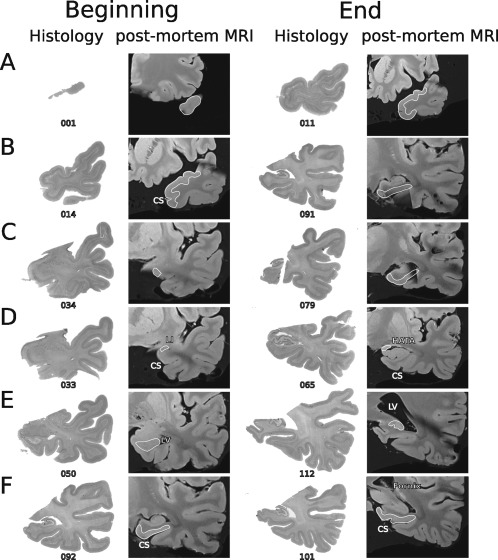
Correspondence between MRI and histology. Example of the correspondence between MTL anatomical landmarks as depicted in post‐mortem MRI scans and neuroanatomical cytoarchitectonic series after processing the same case. Columns from left to right show the beginning (first two columns) and end (last two columns) of each MTL structure on histological sections and on the corresponding post‐mortem T1 MRI slices. Numbers represent the histological section number from the temporal pole (distance between two neighbouring sections: 0.5 mm). (A) Temporopolar cortex, (B) perirhinal cortex, (C) entorhinal cortex, (D) amygdala, (E) hippocampus, (F) posterior parahippocampal cortex. CS, collateral sulcus; LI, limen insulae; LV, lateral ventricle; HATA, hippocampal‐amygdaloid transitional area.
Figure 3.
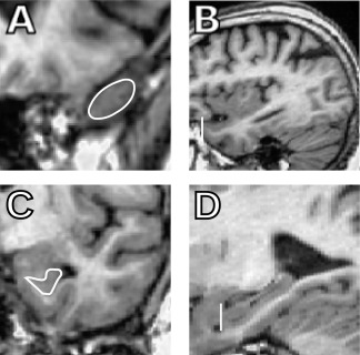
Sagittal views help the identification of some landmarks. The sagittal views [(B) temporal pole (TP), (D) hippocampus (HC)] are especially helpful when defining the beginning of the temporal pole and the hippocampus that can be difficult to localize on the coronal views [(A) TP and (C) HC].
Figure 4.
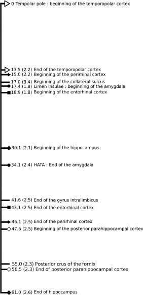
Distances of the beginning and end of each medial temporal lobe (MTL) structures and neuroanatomical landmarks from the beginning of the temporal pole. Distance in millimeters were measured and averaged (±SD) on the 26 in vivo MRI. The different symbols indicate the beginning and end of the different MTL structures (open triangle: temporopolar cortex; full triangle: perirhinal cortex; dot: amygdala; square: entorhinal cortex; full diamond: hippocampus; open diamond: posterior parahippocampal cortex) while a lack of symbols indicate additional useful neuroanatomical landmarks (beginning of the collateral sulcus, end of the gyrus intralimbicus, and posterior crus of the fornix).
Figure 5.
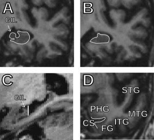
Help for the identification of the end of the gyrus intralimbicus (GIL) and the collateral sulcus on MRI. (A) Last coronal slice containing the GIL and (B) first slice without the GIL. (C) Sagittal view of the hippocampus that helps identifying the end of the GIL. The vertical line indicates the slice that corresponds to the coronal slice shown in Panel B. (D) Coronal slice with the five temporal gyri on which the collateral sulcus can easily be identified between the parahippocampal gyrus and the fusiform gyrus; from this point, the collateral sulcus can be followed anteriorly until its rostralmost extreme. GIL, gyrus intralimbicus; STS, superior temporal gyrus; MTS, middle temporal gyrus; ITS, inferior temporal gyrus; FG, fusiform gyrus; PHG, parahippocampal gyrus; CS, collateral sulcus.
Figure 1 describes a step‐by‐step protocol to identify the different MTL regions on MRI. A template form (Supporting Information Fig. S1) is proposed in the supplemental information to easily keep trace of the identification of landmarks required for the complete protocol. A common difficulty in setting the rostro‐caudal limits of these structures is the partial volume effect. To overcome this problem and increase the consistency of the landmark identification, we chose the slice as first or last if it surely contained the given anatomical landmark. The interrater and intrarater intraclass correlation coefficients for the identification of the boundaries were 0.85 and 0.92, respectively.
DISCUSSION
Here we described anatomical landmarks for the identification of the rostro‐caudal boundaries of the MTL structures on coronal MRI. This protocol is based on cytoarchitectonic analysis of serial sections throughout the temporal lobe designed to identify the whole set of the MTL structures on MRI. Most of the segmentation protocols do not provide boundaries for the MTL cortical regions restricting the researchers and clinicians to the examination of the hippocampus and the amygdala [e.g., Chupin et al., 2009; for review see Geuze et al., 2005; Konrad et al., 2009]. Only few studies described a method for the volumetric segmentation of all the MTL regions [Bonilha et al., 2004; Pruessner et al., 2000, 2002]. However, these segmentations are based on histological findings, sometimes compared to MRI data, reported by other groups [Insausti et al., 1998a; Van Hoesen et al., 2000; Watson et al., 1992], and often combines different protocols. This impeded the authors to compare directly the MRI landmarks to the underlying cytoarchitectony. In contrast, in the present study, the cytoarchitectonic boundaries were defined on the same brains as the anatomical MRI landmarks, and thus provides a higher precision when used for the MRI segmentation.
Furthermore, these boundaries were based on the cytoarchitectonic examination of a large number of human brains. This makes them highly representative of the adult population, in contrast to the atlas of a single brain [Duvernoy, 1988] or the probabilistic atlas based on 10 brains [Amunts et al., 2005].
The protocol described here is an extension of that previously developed for the temporopolar, perirhinal, and entorhinal cortices by Insausti et al. 1998a now including the boundaries of the amygdala, hippocampus and posterior parahippocampal cortex. The previously defined boundaries are confirmed in higher number of cases, showing the reliability of these MR landmarks.
This completed protocol now allows reliable investigations of the all the MTL structures relevant to memory function and neuropsychiatric diseases. It nonetheless requires some training to accurately locate some anatomical features, especially the beginning of the CS. As shown by the high interrater correlation coefficient, after familiarisation with the basic neuroanatomy of the MTL, identification of the MTL landmarks is reliable. Furthermore, identification between raters differed from only one MRI slice for most of the boundaries. Considering the size of the MTL structures, this single slice would represent only a small part of their volumes. It could be argued that the interrater reliability is not as strong as for other segmentation protocols. It has, however, been demonstrated that the landmarks we similarly defined for the entorhinal cortex [Insausti et al., 1998a] were more sensitive to reveal the structure‐function relationships than those proposed in other protocols despite higher interrater reliability in the latter [Price et al., 2010]. This highlights the advantage of histological examination over the only MRI‐based definition as the anatomical reference for the boundary definition, even if the MRI‐based landmarks are easier to apply or more reliable among raters. Finally, our step‐by‐step protocol can be applied to any MRI and can be used after simply visualizing the MRI without the need of advanced image processing.
In conclusion, the rostro‐caudal boundaries described here can help the functional investigations of the MTL regions, and the clinical examination of neuropsychiatric disorders affecting either or both social behavior or memory and learning. This could further improve the understanding of the role of these regions in cognitive processes.
Supporting information
Supporting Information
ACKNOWLEDGMENTS
We acknowledge the excellent technical help of Carmen Ruiz, María Luisa Ramos y Mercedes Iñiguez de Onzoño, as well as the staff of the Human Neuroanatomy Laboratory. We would like to thank Dr. J. Florensa (Servicio de Radiodiagnóstico, Hospital Nacional de Parapléjicos, Toledo, Spain) for the 3T imaging in post‐mortem cases.
REFERENCES
- Adolphs R (2010): What does the amygdala contribute to social cognition? Ann N Y Acad Sci 1191:42–61. [DOI] [PMC free article] [PubMed] [Google Scholar]
- Aggleton J (1992): The functional effects of amygdala lesions in humans: A comparison with findings from monkeys. In: Aggleton JP, editor. The Amygdala: Neurobiological aspects of emotion, memory, and mental dysfunction. New York: Wiley‐Liss. pp 485–503.
- Aggleton J (2000): The Amygdala. A Functional Analysis.Oxford:Oxford University Press; 690 p. [Google Scholar]
- Alvarado MC, Bachevalier J (2005): Comparison of the effects of damage to the perirhinal and parahippocampal cortex on transverse patterning and location memory in rhesus macaques. J Neurosci 25:1599–1609. [DOI] [PMC free article] [PubMed] [Google Scholar]
- Amaral DG (2003): The amygdala, social behavior, and danger detection. Ann N Y Acad Sci 1000:337–347. [DOI] [PubMed] [Google Scholar]
- Amunts K, Kedo O, Kindler M, Pieperhoff P, Mohlberg H, Shah NJ, Habel U, Schneider F.Zilles K (2005): Cytoarchitectonic mapping of the human amygdala, hippocampal region and entorhinal cortex: Intersubject variability and probability maps. Anat Embryol (Berl) 210:343–352. [DOI] [PubMed] [Google Scholar]
- Bartzokis G, Altshuler LL, Greider T, Curran J, Keen B, Dixon WJ (1998): Reliability of medial temporal lobe volume measurements using reformatted 3D images. Psychiatry Res 82:11–24. [DOI] [PubMed] [Google Scholar]
- Bernasconi N, Bernasconi A, Caramanos Z, Antel SB, Andermann F, Arnold DL (2003): Mesial temporal damage in temporal lobe epilepsy: A volumetric MRI study of the hippocampus, amygdala and parahippocampal region. Brain 126:462–469. [DOI] [PubMed] [Google Scholar]
- Binder JR, Desai RH, Graves WW, Conant LL (2009): Where is the semantic system? A critical review and meta‐analysis of 120 functional neuroimaging studies. Cereb Cortex 19:2767–2796. [DOI] [PMC free article] [PubMed] [Google Scholar]
- Blaizot X, Landeau B, Baron JC, Chavoix C (2000): Mapping the visual recognition memory network with PET in the behaving baboon. J Cereb Blood Flow Metab 20:213–219. [DOI] [PubMed] [Google Scholar]
- Blaizot X, Meguro K, Millien I, Baron JC, Chavoix C (2002): Correlations between visual recognition memory and neocortical and hippocampal glucose metabolism after bilateral rhinal cortex lesions in the baboon: Implications for Alzheimer's disease. J Neurosci 22:9166–9170. [DOI] [PMC free article] [PubMed] [Google Scholar]
- Bonilha L, Kobayashi E, Cendes F, Min Li L (2004): Protocol for volumetric segmentation of medial temporal structures using high‐resolution 3‐D magnetic resonance imaging. Hum Brain Mapp 22:145–154. [DOI] [PMC free article] [PubMed] [Google Scholar]
- Braak H, Braak E (1991): Neuropathological stageing of Alzheimer‐related changes. Acta Neuropathol 82:239–259. [DOI] [PubMed] [Google Scholar]
- Chupin M, Hammers A, Liu RSN, Colliot O, Burdett J, Bardinet E, Duncan JS, Garnero L, Lemieux L (2009): Automatic segmentation of the hippocampus and the amygdala driven by hybrid constraints: Method and validation. Neuroimage 46:749–761. [DOI] [PMC free article] [PubMed] [Google Scholar]
- Davachi L (2006): Item, context and relational episodic encoding in humans. Curr Opin Neurobiol 16:693–700. [DOI] [PubMed] [Google Scholar]
- Davachi L, Wagner AD (2002): Hippocampal contributions to episodic encoding: Insights from relational and item‐based learning. J Neurophysiol 88:982–990. [DOI] [PubMed] [Google Scholar]
- Ding SL, Van Hoesen GW (2010): Borders, extent, and topography of human perirhinal cortex as revealed using multiple modern neuroanatomical and pathological markers. Hum Brain Mapp 31:1359–1379. [DOI] [PMC free article] [PubMed] [Google Scholar]
- Duvernoy H (1988): Anatomy of the Hippocampus. The Human Hippocampus, an Atlas of Applied Anatomy.New York:Springer‐Verlag; pp25–43. [Google Scholar]
- Eichenbaum H, Dudchenko P, Wood E, Shapiro M, Tanila H (1999): The hippocampus, memory, and place cells: Is it spatial memory or a memory space? Neuron 23:209–226. [DOI] [PubMed] [Google Scholar]
- Ekstrom AD, Kahana MJ, Caplan JB, Fields TA, Isham EA, Newman EL, Fried I (2003): Cellular networks underlying human spatial navigation. Nature 425:184–188. [DOI] [PubMed] [Google Scholar]
- Epstein R (2005): The cortical basis of visual scene processing. Vis Cognit 12:954–978. [Google Scholar]
- Gallagher M, Chiba AA (1996): The amygdala and emotion. Curr Opin Neurobiol 6:221–227. [DOI] [PubMed] [Google Scholar]
- Geuze E, Vermetten E, Bremner JD (2005): MR‐based in vivo hippocampal volumetrics. Part 2. Findings in neuropsychiatric disorders. Mol Psychiatry 10:160–184. [DOI] [PubMed] [Google Scholar]
- Hodges JR, Patterson K, Oxbury S, Funnell E (1992): Semantic dementia. Progressive fluent aphasia with temporal lobe atrophy. Brain 115(Pt 6):1783–1806. [DOI] [PubMed] [Google Scholar]
- Insausti R, Amaral D (2004): Hippocampal formation In: Paxinos G, Mai JK, editors. The Human Nervous System, 2nd ed. Amsterdam:Elsevier; pp871–914. [Google Scholar]
- Insausti R, Insausti AM, Mansilla F, Abizanda P, Artacho‐Pérula E, Arroyo‐Jimenez MM, Martinez‐Marcos A, Marcos P y Muñoz‐Lopez M (2003).The human parahippocampal gyrus. anatomical and MRI correlates. Soc Neurosci Abs 935.5. [Google Scholar]
- Insausti R, Tuñón T, Sobreviela T, Insausti AM, Gonzalo LM (1995): The human entorhinal cortex: A cytoarchitectonic analysis. J Comp Neurol 355:171–198. [DOI] [PubMed] [Google Scholar]
- Insausti R, Juottonen K, Soininen H, Insausti AM, Partanen K, Vainio P, Laakso MP, Pitkanen A (1998a): MR volumetric analysis of the human entorhinal, perirhinal, and temporopolar cortices. AJNR Am J Neuroradiol 19:659–671. [PMC free article] [PubMed] [Google Scholar]
- Insausti R, Insausti AM, Sobreviela T, Salinas A, Martinez‐Penuela JM (1998b): Human medial temporal lobe in aging: Anatomical basis of memory preservation. Microsc Res Tech 43:8–15. [DOI] [PubMed] [Google Scholar]
- Juottonen K, Laakso MP, Insausti R, Lehtovirta M, Pitkanen A, Partanen K, Soininen H (1998): Volumes of the entorhinal and perirhinal cortices in Alzheimer's disease. Neurobiol Aging 19:15–22. [DOI] [PubMed] [Google Scholar]
- Kapur N, Ellison D, Smith MP, McLellan DL, Burrows EH (1992): Focal retrograde amnesia following bilateral temporal lobe pathology. A neuropsychological and magnetic resonance study. Brain 115(Pt 1):73–85. [DOI] [PubMed] [Google Scholar]
- Konrad C, Ukas T, Nebel C, Arolt V, Toga AW, Narr KL (2009): Defining the human hippocampus in cerebral magnetic resonance images–an overview of current segmentation protocols. Neuroimage 47:1185–1195. [DOI] [PMC free article] [PubMed] [Google Scholar]
- Laakso MP, Partanen K, Riekkinen P, Lehtovirta M, Helkala EL, Hallikainen M, Hanninen T, Vainio P, Soininen H (1996): Hippocampal volumes in Alzheimer's disease, Parkinson's disease with and without dementia, and in vascular dementia: An MRI study. Neurology 46:678–681. [DOI] [PubMed] [Google Scholar]
- Malkova L, Mishkin M (2003): One‐trial memory for object‐place associations after separate lesions of hippocampus and posterior parahippocampal region in the monkey. J Neurosci 23:1956–1965. [DOI] [PMC free article] [PubMed] [Google Scholar]
- Malkova L, Bachevalier J, Mishkin M, Saunders RC (2001): Neurotoxic lesions of perirhinal cortex impair visual recognition memory in rhesus monkeys. Neuroreport 12:1913–1917. [DOI] [PubMed] [Google Scholar]
- Meguro K, Blaizot X, Kondoh Y, Le Mestric C, Baron JC, Chavoix C (1999): Neocortical and hippocampal glucose hypometabolism following neurotoxic lesions of the entorhinal and perirhinal cortices in the non‐human primate as shown by PET. Implications for Alzheimer's disease. Brain 122(Pt 8):1519–1531. [DOI] [PubMed] [Google Scholar]
- Meunier M, Bachevalier J (2002): Comparison of emotional responses in monkeys with rhinal cortex or amygdala lesions. Emotion 2:147–161. [DOI] [PubMed] [Google Scholar]
- Meunier M, Bachevalier J, Mishkin M, Murray EA (1993): Effects on visual recognition of combined and separate ablations of the entorhinal and perirhinal cortex in rhesus monkeys. J Neurosci 13:5418–5432. [DOI] [PMC free article] [PubMed] [Google Scholar]
- Moser EI, Moser MB (2008): A metric for space. Hippocampus 18:1142–1156. [DOI] [PubMed] [Google Scholar]
- Ohman A, Mineka S (2001): Fears, phobias, and preparedness: Toward an evolved module of fear and fear learning. Psychol Rev 108:483–522. [DOI] [PubMed] [Google Scholar]
- O'Keefe J, Dostrovsky J (1971): The hippocampus as a spatial map. Preliminary evidence from unit activity in the freely‐moving rat. Brain Res 34:171–175. [DOI] [PubMed] [Google Scholar]
- Pessoa L (2010): Emergent processes in cognitive‐emotional interactions. Dialogues Clin Neurosci 12:433–448. [DOI] [PMC free article] [PubMed] [Google Scholar]
- Pitkanen A, Kelly JL, Amaral DG (2002): Projections from the lateral, basal, and accessory basal nuclei of the amygdala to the entorhinal cortex in the macaque monkey. Hippocampus 12:186–205. [DOI] [PubMed] [Google Scholar]
- Price CC, Wood MF, Leonard CM, Towler S, Ward J, Montijo H, Kellison I, Bowers D, Monk T, Newcomer JC, Schmalfuss I (2010): Entorhinal cortex volume in older adults: Reliability and validity considerations for three published measurement protocols. J Int Neuropsychol Soc 16:846–855. [DOI] [PMC free article] [PubMed] [Google Scholar]
- Pruessner JC, Li LM, Serles W, Pruessner M, Collins DL, Kabani N, Lupien S, Evans AC (2000): Volumetry of hippocampus and amygdala with high‐resolution MRI and three‐dimensional analysis software: Minimizing the discrepancies between laboratories. Cereb Cortex 10:433–442. [DOI] [PubMed] [Google Scholar]
- Pruessner JC, Kohler S, Crane J, Pruessner M, Lord C, Byrne A, Kabani N, Collins DL, Evans AC (2002): Volumetry of temporopolar, perirhinal, entorhinal and parahippocampal cortex from high‐resolution MR images: Considering the variability of the collateral sulcus. Cereb Cortex 12:1342–1353. [DOI] [PubMed] [Google Scholar]
- Rauchs G, Blaizot X, Giffard C, Baron JC, Insausti R, Chavoix C (2006): Imaging visual recognition memory network by PET in the baboon: Perirhinal cortex heterogeneity and plasticity after perirhinal lesion. J Cereb Blood Flow Metab 26:301–309. [DOI] [PubMed] [Google Scholar]
- Rolls E (1992): Neurophysiology and functions of the primate amygdala In: Aggleton JP, editor. The Amygdala: Neurobiological aspects of emotion, memory, and mental dysfunction.New York:Wiley‐Liss; pp143–165. [Google Scholar]
- Schumann CM, Hamstra J, Goodlin‐Jones BL, Lotspeich LJ, Kwon H, Buonocore MH, Lammers CR, Reiss AL, Amaral DG (2004): The amygdala is enlarged in children but not adolescents with autism; the hippocampus is enlarged at all ages. J Neurosci 24:6392–6401. [DOI] [PMC free article] [PubMed] [Google Scholar]
- Squire LR (1992): Memory and the hippocampus: A synthesis from findings with rats, monkeys, and humans. Psychol Rev 99:195–231. [DOI] [PubMed] [Google Scholar]
- Squire LR, Stark CEL, Clark RE (2004): The medial temporal lobe. Annu Rev Neurosci 27:279–306. [DOI] [PubMed] [Google Scholar]
- Suzuki WA, Amaral DG (1994): Perirhinal and parahippocampal cortices of the macaque monkey: Cortical afferents. J Comp Neurol 350:497–533. [DOI] [PubMed] [Google Scholar]
- Suzuki WA, Eichenbaum H (2000): The neurophysiology of memory. Ann N Y Acad Sci 911:175–191. [DOI] [PubMed] [Google Scholar]
- Suzuki WA, Miller EK, Desimone R (1997): Object and place memory in the macaque entorhinal cortex. J Neurophysiol 78:1062–1081. [DOI] [PubMed] [Google Scholar]
- Thangavel R, Van Hoesen GW, Zaheer A (2008): Posterior parahippocampal gyrus pathology in Alzheimer's disease. Neuroscience 154:667–676. [DOI] [PMC free article] [PubMed] [Google Scholar]
- Van Hoesen GW, Augustinack JC, Dierking J, Redman SJ, Thangavel R (2000): The parahippocampal gyrus in Alzheimer's disease. Clinical and preclinical neuroanatomical correlates. Ann N Y Acad Sci 911:254–274. [DOI] [PubMed] [Google Scholar]
- von Gunten A, Ron MA (2004): Hippocampal volume and subjective memory impairment in depressed patients. Eur Psychiatry 19:438–440. [DOI] [PubMed] [Google Scholar]
- Watson C, Andermann F, Gloor P, Jones‐Gotman M, Peters T, Evans A, Olivier A, Melanson D, Leroux G (1992): Anatomic basis of amygdaloid and hippocampal volume measurement by magnetic resonance imaging. Neurology 42:1743–1750. [DOI] [PubMed] [Google Scholar]
Associated Data
This section collects any data citations, data availability statements, or supplementary materials included in this article.
Supplementary Materials
Supporting Information