

Abstract
The functional role of the left ventral occipito‐temporal cortex (vOT) in visual word processing has been studied extensively. A prominent observation is higher activation for unfamiliar but pronounceable letter strings compared to regular words in this region. Some functional accounts have interpreted this finding as driven by top‐down influences (e.g., Dehaene and Cohen [2011]: Trends Cogn Sci 15:254–262; Price and Devlin [2011]: Trends Cogn Sci 15:246–253), while others have suggested a difference in bottom‐up processing (e.g., Glezer et al. [2009]: Neuron 62:199–204; Kronbichler et al. [2007]: J Cogn Neurosci 19:1584–1594). We used dynamic causal modeling for fMRI data to test bottom‐up and top‐down influences on the left vOT during visual processing of regular words and unfamiliar letter strings. Regular words (e.g., taxi) and unfamiliar letter strings of pseudohomophones (e.g., taksi) were presented in the context of a phonological lexical decision task (i.e., “Does the item sound like a word?”). We found no differences in top‐down signaling, but a strong increase in bottom‐up signaling from the occipital cortex to the left vOT for pseudohomophones compared to words. This finding can be linked to functional accounts which assume that the left vOT contains neurons tuned to complex orthographic features such as morphemes or words [e.g., Dehaene and Cohen [2011]: Trends Cogn Sci 15:254‐262; Kronbichler et al. [2007]: J Cogn Neurosci 19:1584–1594]: For words, bottom‐up signals converge onto a matching orthographic representation in the left vOT. For pseudohomophones, the propagated signals do not converge, but (partially) activate multiple orthographic word representations, reflected in increased effective connectivity. Hum Brain Mapp 35:1668–1680, 2014. © 2013 Wiley Periodicals, Inc.
Keywords: fMRI, brain connectivity, dynamic causal modeling, visual recognition, reading
INTRODUCTION
Patient studies showed that the left ventral occipito‐temporal cortex (vOT) is essential for fast and efficient reading [e.g., Cohen et al., 2003; Gaillard et al., 2007; Roberts et al., 2012]. For the last decade, the functional role of this area has been a central theme in the field of neurocognitive reading research. Dehaene and Cohen [2011; see also Cohen et al., 2000; Dehaene et al., 2005] have proposed that the left vOT hosts a visual word form area (VWFA) which contains neurons tuned to orthographic features of words. These features are mainly sublexical in nature, as for example, letter‐pairings (bigrams), multiletter sequences (morphemes), or short words. Based on Dehaene and Cohens theoretical framework, others suggested that some neurons in the VWFA are also tuned to lexical whole‐word representations [e.g., Glezer et al., 2009; Kronbichler et al., 2007]. A contrasting account of the left vOT was proposed by Price and Devlin [2011; see also Price and Devlin, 2003]. In their view, the left vOT's neurons are not specifically tuned to orthographic features. The functional role of the left vOT is to integrate visual inputs with higher level associations such as speech sounds and meaning. Orthographic representations emerge from the interaction of bottom‐up and top‐down influences.
A classical way to probe the functional role of the left vOT is the comparison between regular words and unfamiliar letter strings. Multiple evidence shows that unfamiliar but pronounceable letter strings (e.g., low‐frequency words, pseudowords or pseudohomophones) lead to higher activation in the left vOT compared to regular words [see Jobard et al., 2003 for a meta‐analysis]. This pattern can be found for all tasks which require (and enable) a complete reading of the letter string, like for example reading aloud [see Dehaene and Cohen, 2011 for a discussion]. In the mentioned functional accounts, stronger activation for unfamiliar letter strings in the left vOT is mainly interpreted as driven by top‐down influences. According to Dehaene and Cohen [2011, p.457], neurons in the left vOT are equally tuned to regular words and unfamiliar letter strings (if pronouncable and matched for sublexical orthographic features). Still, increased activation for unfamiliar letter strings is observed because these items receive stronger top‐down activation or require more processing in general. According to Price and Devlin [2011], neurons in the left vOT are neither tuned to regular words nor to unfamiliar letter strings. Activation is higher for unfamiliar letter strings than for words because—although both receive top‐down activation—there is a greater “prediction error” for unfamiliar letter strings. “Predictions” denote top‐down activations from phonological and semantic areas which are based on the prior experience with a stimulus; they are needed to resolve uncertainty about the sensory input (letter string).
A number of imaging studies compared regular words to pseudohomophones (e.g., Taxi compared to Taksi). Pseudohomophones are of interest for testing the orthographic tuning of the left vOT: although they are orthographically unfamiliar, they do correspond to a phonologically familiar form (e.g., in German, Taksi sounds just like Taxi). Nevertheless, studies found higher activation for pseudohomophones compared to words in the left vOT. This pattern was consistently reported across a variety of different tasks, such as reading aloud [Borowski et al., 2006], reading silently [Kronbichler et al., 2009], making orthographic decisions [i.e., “Is the item an existing word?”; Twomey et al., 2011] and making phonological lexical decisions [i.e., “Does the item sound like a word?”; Bruno et al., 2008; Kronbichler et al., 2007; van der Mark et al., 2009]. The finding of relatively higher activation for pseudohomophones in the left vOT cannot be immediately explained in terms of top‐down influences. For example, in the context of a phonological lexical decision (Does the item sound like a word?), both pseudohomophones and words are phonologically familiar, are associated with the same meaning, and receive a “yes” response in the task. An alternative interpretation of this finding—which emphasizes differences in bottom‐up rather than top‐down signaling—was proposed by Kronbichler et al. [2007; see also Glezer et al., 2009]. This interpretation is based on the assumption that the left vOT hosts not only orthographic representations of morphemes and small words [c.f., Dehaene and Cohen, 2011], but also orthographic representations of whole words. In this perspective, increased activation for orthographically unfamiliar letter strings can be interpreted as a bottom‐up activation of multiple orthographic word representations. For example, visual encoding of the letter‐sequence t‐a‐k‐s‐i (pseudohomophone) may lead to a (partial) activation of the orthographic representations take, table, taxi, sit, sister, and so on. In contrast, encoding of the letter‐sequence t‐a‐x‐i may specifically activate one orthographic representation (taxi), which is reflected by more precise neural signaling and less overall activity.
The present study follows up the finding of higher activation for pseudohomophones compared to words in the left vOT. We rely on dynamic causal modeling [DCM, Friston et al., 2003] to explain this finding in terms of bottom‐up versus top‐down influences on the left vOT. Identification of these interactions contributes to the clarification of functional accounts of the left vOT. DCM is a method to study effective connectivity, that is, directed interactions between brain regions. It affords mechanistic explanations of how activity in one brain area is driven (i.e., caused) by influences from other areas. The left vOT is the most consistently featured brain region in effective connectivity studies on visual word processing [Bitan et al., 2005, 2006, 2007, 2008; Booth et al., 2008; Cao et al., 2008; Heim et al., 2009; Mechelli et al., 2005; Nakamura et al., 2007; Seghier et al., 2010; Sonty et al., 2007]. Most studies conceptualized the left vOT as the starting point of visual word processing in the brain, and focused on how it is forwarding activity to higher order language areas, for example, left inferior frontal areas. DCM studies could establish that the left vOT is substantially involved in driving brain activity in left inferior frontal areas, and that this driving adapts to differential task and stimulus properties [e.g., Bitan et al., 2005, 2006, 2008; Heim et al., 2009; Mechelli et al., 2005; Sonty et al., 2007]. In contrast to occipito‐temporal “forward” connectivity, relatively little attention was devoted to occipito‐temporal interactions with low‐level visual processing regions in the occipital cortex. A few DCM studies on visual word processing have analyzed occipito‐temporal brain connectivity and did select an occipital brain region as starting point for their analysis [Booth et al., 2008; Richardson et al., 2011; Seghier et al., 2012]. Two studies [Booth et al., 2008; Richardson et al., 2011] showed that signaling from the occipital cortex to the vOT increases for processing words (and sentences) compared to nonlinguistic visual material (e.g., false‐fonts, line‐strings). These findings highlight that changes in bottom‐up signaling are relevant for the functioning of the left vOT.
We focused our DCM analysis on the question how bottom‐up versus top‐down influences are driving activation for pseudohomophones (relative to words) in the left vOT. To test this question, we analyzed fMRI data for words and pseudohomophones in a phonological lexical decision task [i.e., “Does the item sound like a word?”; Kronbichler et al., 2007]. We constructed the simplest model for this question, consisting of three brain areas: One low‐level visual area in the occipital cortex, one area in the left vOT, and one higher level language area in the left inferior frontal gyrus. Using a simple three‐area network allowed us to perform a systematic (i.e., exhaustive) comparison of different bottom‐up and top‐down connectivity architectures by means of Bayesian Model Comparison [e.g., Penny et al., 2010]. We created 64 different dynamic causal models, each defining a distinct set of top‐down and bottom‐up influences operating on the left vOT. The critical difference between models was the way how orthographic familiarity (the difference between words and pseudohomophones, i.e., Taxi versus Taksi) changed effective connectivity. If neurons in the left vOT process pre‐lexical orthographic features [e.g., bigrams or morphemes, Dehaene and Cohen, 2011] or low‐level visual features [Price and Devlin, 2011], bottom‐up processing of words and pseudohomophones matched for these features can expected to be the same. Therefore, an activation difference between words and pseudohomophones in the left vOT should be driven by top‐down influences. In contrast, if neurons in the left vOT also process lexical orthographic features [i.e., whole‐words, Glezer et al., 2009; Kronbichler et al., 2007], an activation difference between words and pseudohomophones may also reflect a difference in bottom‐up signaling.
METHODS
Participants
FMRI data were acquired from 24 German‐speaking volunteers (21 males). All participants (age 15‐34 years) were right handed and reported no history of neurological disease or reading difficulty. Informed consent was provided by each participant. For adolescents, consent was also provided by a parent. The study was approved by the ethical committee of the University of Salzburg.
Stimuli and Task
The 180 stimuli consisted of 60 regular words in the form of German nouns, 60 pseudohomophones derived from the words, and 60 pseudowords. Examples for the three item types are Taxi—Taksi—Tazi or Chaos—Kaos—Kuse. Regular words consisted of 4–9 letters and began with a consonant (in upper case following German spelling convention for nouns). Pseudohomophones did not differ from the regular words in number of letters, syllables, bigram frequency, and in number of orthographic neighbors. Item characteristics are listed in Supporting Information Table S1. The mean frequency of 86 occurrences per million according to the CELEX database [Baayen, Piepenbrock, and van Rijn, 1993] indicates that the majority of words was of moderate to high frequency. Pseudowords were generated in such a way that they could not be distinguished from pseudohomophones by superficial characteristics such as absence of vowel letters or length.
A fast event‐related design was used. Each item was displayed for 1600 ms with an interstimulus interval of 2100 ms during which a fixation cross was shown. The 180 stimuli were presented in two runs of 90 items, each composed of 30 items per stimulus type. In addition, 10 null‐events of 3700 ms duration with a fixation cross were included in each run. The order of the 90 stimuli and of the 10 null events within each run was determined by a genetic algorithm [Wager and Nichols, 2003]. We used two different pseudo‐randomized stimulus sequences, which were changed from participant to participant. A critical feature for creating the sequences was the ordering of regular words (e.g., Taxi) and their corresponding pseudohomophones (e.g., Taksi). When in sequence one a regular word was presented before its corresponding pseudohomophone, then this order was reversed in sequence two. Change of the sequence from participant to participant ascertained that a regular word was equally often presented before and after its corresponding pseudohomophone. Participants were familiarized with the phonological lexical decision task (i.e., “Does the item sound like a word?”) and with the response mode outside the scanner. Participants responded with the index finger (yes) and middle finger (no) of their right hand. Stimulus delivery and response registration were controlled by Presentation (Neurobehavioral Systems Inc., Albany, CA, USA).
fMRI Data Acquisition and Analysis
During each of the two runs, 190 functional images sensitive to BOLD contrast were acquired with a T 2*‐weighted EPI sequence (TE 40 ms, TR 2000 ms, FA 86°, 21 slices with a thickness of 6 mm, 220 mm FOV with a 64 × 64 matrix resulting in 3.44 × 3.44 mm in plane resolution). A high‐resolution (1 × 1 × 1.3 mm) structural scan was acquired from each participant with a T 1‐weighted MPRAGE sequence. A Philips 1.5‐T Intera Scanner (Philips Medical System, Best, The Netherlands) was used for MR imaging.
For consistency with a previous publication on the present data [Kronbichler et al., 2007], we used SPM2 for data preprocessing and voxel‐based statistics (http://www.fil.ion.ucl.ac.uk/spm). The subsequent analyses with DCM were performed with SPM5 and SPM8 (individual DCMs were generated in SPM5, model comparison was performed with recent methods only available in SPM8). Functional images were realigned and unwarped, slice time corrected, and co‐registered to the high‐resolution structural image. The structural image was normalized to the Montreal Neurological Institute T1 template image, and the resulting parameters were used for normalization of the functional images, which were resampled to isotropic 3‐mm three voxels and smoothed with a 9‐mm full width at half maximum Gaussian kernel. Statistical analysis was performed in a two‐stage random‐effects model. In the subject‐specific first‐level model, each stimulus type was modeled by a canonical hemodynamic response function and its temporal derivative. The few incorrectly answered and missed items were modeled as covariates of no interest. The functional data in these first‐level models were high‐pass filtered with a cutoff of 128 sec, and corrected for autocorrelation by an AR(1) model [Friston et al., 2002]. In these first‐level models, the parameter estimates reflecting signal change for each stimulus type versus fixation baseline (which consisted of the interstimulus interval and the null events) were calculated in the context of a general linear model [see Henson, 2004]. Contrasts of interest were obtained for each participant from these first‐level parameter estimates and used in a second‐level random effects model. For consistency with a previous publication on the present data results were obtained with a voxelwise q < 0.01, corrected for multiple comparisons using the false discovery rate [FDR; Genovese, Lazar, and Nichols, 2002] and a minimum cluster extent of five voxels [see Kronbichler et al., 2007 for details]. Regions entering our DCM analysis were selected from these corrected results (see Supporting Information Table S2). For the display of activation maps in Figure 1, however, we used a more liberal threshold (uncorrected P < 0.001 and a cluster extent threshold of 20 voxels).
Figure 1.
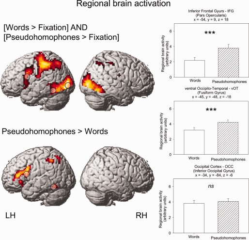
Top: Regions showing activation for the conjunction words > fixation and pseudohomophones > fixation. Bottom: Regions showing increased activation for pseudohomophones > words. Results are shown at a voxelwise threshold of P < 0.001 and minimum extent of 20 voxels. Bar‐charts report brain activity estimates (M; SEM) for regions of interests. [Color figure can be viewed in the online issue, which is available at http://wileyonlinelibrary.com]
Dynamic Causal Modeling
DCM investigates how brain regions interact with each other during different experimental contexts [Friston et al., 2003]. The strength and direction of interactions are captured by the parameters of a DCM, which define its dynamic functional architecture. The number and arrangement of parameters in each model are user‐defined. Parameters of a model are then adjusted in an iterative manner (Bayesian parameter estimation) so that the predicted responses match the observed responses as closely as possible. There are three sets of parameters that model neuronal activity: (1) Parameters that regulate the direct influences of driving inputs on the neuronal activity. Driving inputs correspond to the experimental stimuli in a study, e.g., visual letters. (2) Parameters that regulate the intrinsic (or fixed) connections between areas. These connections reflect the context independent coupling of activity in different regions. (3) Parameters that regulate modulatory effects, which reflect context‐dependent changes in coupling between areas. This could be, for example, effects of stimulus properties, or effects of learning on the coupling between areas. In DCM, parameter estimates are expressed in terms of the rate of change of neural activity in one area that is associated with activity in another area (i.e., rate constants), and are in units of s−1, (hertz). For example, if effective connectivity from area A to area B is 0.10 s−1, this means that, per unit time, the increase in activity in B corresponds to 10% of the activity in A [den Ouden, 2009]. To explain regional BOLD responses, the DCM of neural activity is combined with a biophysical forward model of hemodynamic responses.
Brain Regions in the Model
Time series from regions of interest were used for the DCM analysis. Locations of the regions entering into the DCM analysis were based on the results of the voxel‐based group analysis. As a low‐level visual processing region, we selected an occipital cortex region (x = −39, y = −84, z = −6) from from the conjunction of the contrasts words versus fixation and pseudohomophones versus fixation. The location of our occipital area corresponds to the location found for visual letter string processing in meta‐analyses [at around y = −80; Bolger and Perfetti, 2005; Jobard et al., 2003]. From the contrast of pseudohomophones versus words (see Supporting Information Table 2), we selected a left occipito‐temporal region (left vOT: x = −45, y = −48, z = −18) and a left inferior frontal gyrus region (IFG: x = −54, y = 9, z = 18). To obtain subject‐specific activation maxima, we calculated the contrast of words and pseudohomophones versus fixation for the OCC region, and the contrast of pseudohomophones minus words for the left vOT and left inferior frontal regions. These contrasts were computed within small volumes of 10 mm radius around the group maxima, and were thresholded at an uncorrected threshold of P < 0.05 [c.f. Mechelli et al., 2005; Heim et al., 2009]. From the subject specific activation maxima, time series data (principal eigenvariates) were extracted from regions of interest (6 mm radius), and adjusted to the effects of interest contrast. Time series data were concatenated over the sessions, and two regressors of no interest were added to account for session effects. In addition, the few incorrectly answered and missed items were modeled as regressors of no interest, so that only correct responses were considered in the DCM analysis. Five of 24 subjects did not show activity in at least one of the target areas. The remaining 19 subjects were used for the DCM analysis. Coordinates of the regions of interest for each subject are given in Table 1.
Table 1.
Locations of Regions of Interest entering the DCM analysis (MNI space)
| Subj. | OCC | Lb | d 1 | vOT | Lb | d 2 | IFG | Lb | ||||||
|---|---|---|---|---|---|---|---|---|---|---|---|---|---|---|
| x | y | z | x | y | z | x | y | z | ||||||
| 1 | −42 | −84 | −15 | FFG | 37 | −45 | −48 | −24 | FFG | 69 | −63 | 6 | 15 | POS |
| 2 | −36 | −87 | −9 | IOG | 33 | −45 | −57 | −18 | FFG | 84 | −57 | 15 | 24 | IFO |
| 3 | −36 | −87 | −6 | IOG | 45 | −51 | −45 | −9 | ITG | 49 | −57a | −3a | 15a | POS |
| 4 | −45 | −84 | 0 | MOG | 36 | −48 | −51 | −15 | ITG | 74 | −48 | 15 | 18 | IFO |
| 5 | −39 | −81 | −12 | FFG | 38 | −51 | −45 | −9 | ITG | 65 | −51 | 9 | 27 | IFO |
| 6 | −33 | −81 | −6 | IOG | 27 | −45 | −57 | −12 | IOG | 76 | −63 | 12 | 15 | IFO |
| 7 | −30 | −87 | −9 | IOG | 39 | −51 | −54 | −12 | ITG | 67 | −57 | 9 | 9 | IFO |
| 8 | −33 | −81 | 0 | IOG | 30 | −42 | −54 | −9 | ITG | 71 | −51 | 6 | 27 | PRE |
| 9 | −42 | −81 | −15 | FFG | 39 | −45 | −42 | −12 | ITG | 58 | −54a | 12a | 6a | IFO |
| 10 | −39 | −78 | −12 | FFG | 30 | −45 | −51 | −24 | ITG | 81 | −45a | 9a | 30a | IFO |
| 11 | −39 | −84 | 3 | MOG | 41 | −57a | −48a | −6a | ITG | 52 | −45a | −3a | 18a | ROL |
| 12 | −33 | −87 | 0 | MOG | 39 | −48 | −54 | −15 | ITG | 80 | −57 | 15 | 24 | IFO |
| 13 | −42 | −78 | −12 | IOG | 22 | −48 | −57 | −12 | ITG | 71 | −57 | 9 | 12 | IFO |
| 14 | −27 | −75 | −21 | CBL | 29 | −42 | −51 | −15 | FFG | 74 | −57 | 12 | 21 | IFO |
| 15 | −39 | −90 | −12 | IOG | 33 | −42 | −57 | −12 | FFG | 71 | −45 | 6 | 21 | PRE |
| 16 | −39 | −81 | −9 | IOG | 34 | −39 | −48 | −18 | FFG | 74 | −51 | 9 | 27 | IFO |
| 17 | −39 | −81 | 0 | MOG | 41 | −42 | −48 | −24 | FFG | 76 | −63 | 12 | 18 | IFO |
| 18 | −36 | −87 | 3 | MOG | 46 | −51 | −51 | −21 | ITG | 75 | −45a | 6a | 27a | IFO |
| 19 | −36 | −84 | −15 | LIG | 30 | −39 | −54 | −15 | FFG | 74 | −63 | 9 | 15 | IFO |
| Mean | −38 | −84 | −7 | IOG | 35 | −46 | −51 | −15 | ITG | 70 | −55 | 10 | 19 | IFO |
Radius of search volume was extended to 15 mm; d 1: euclidian distance (mm) between OCC and vOT; d 2: distance between vOT and IFG; Anatomical Labels (Lb): FFG, fusiform gyrus; IOG, inferior occipital gyrus; MOG, middle occipital gyrus; LIG, lingual gyrus; CBL, cerebellum; ITG, inferior temporal gyrus; POS, postcentral gyrus; PRE, precentral gyrus; ROL, Rolandic operculum; IFO, inferior frontal gyrus pars opercularis.
Model Construction
All models were constructed using the same basic architecture: The occipital area served as input region. Both letter strings of words and pseudohomophones (modeled as a single regressor) exerted direct influence on this region. All models included reciprocal intrinsic (fixed) connectivity between the three areas in occipital cortex, left vOT and left inferior frontal gyrus. This basic architecture is shown in Figure 2C and is termed model #1 (null model). The basic model was then extended by additionally modeling changes in connection strength in response to the orthographic familiarity of a letter string. Orthographic familiarity was modeled as a regressor coding the presence of orthographically unfamiliar pseudohomophones. Modulatory effects therefore express how brain connectivity changes when presenting a word in an orthographically unfamiliar form (e.g., taksi) compared to a regular form (e.g., taxi). Our design of modulatory effects was based on the voxelwise results, which showed higher activity for pseudohomophones compared to words in a number of areas, but no areas with higher activity for words compared to pseudohomophones. In order to explore how orthographic familiarity changes connectivity strength, we systematically varied its effect on connectivity. We constructed 64 DCMs, each representing a different way of how brain connectivity is changed. The 64 models are summarized in Figure 2A in a table‐like fashion. Individual examples for models are given in Figure 2C.
Figure 2.
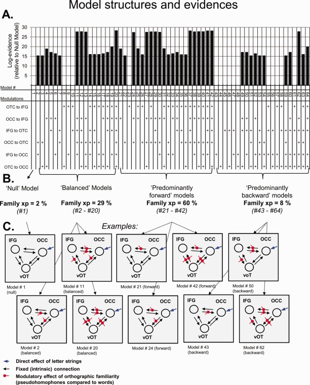
(A) Connectivity structure and log‐model evidence (negative free energy) of the dynamic causal models. Log‐model evidences are relative to the null‐model. Models are ordered after model family (Null, Balanced, Forward, Backward) and model complexity (number of modulatory parameters). (B) Results of the family level inference. Family model evidence given as exceedance probability xP (the probability in % that a particular model family is more likely than any other family). (C) Examples of individual models of each family. [Color figure can be viewed in the online issue, which is available at http://wileyonlinelibrary.com]
Model Selection
To select the optimal model given our data, we used the Bayesian model selection (BMS). We used the most recent BMS procedure published in June 2011 (available in the SPM8 revision #4376). Model selection rests on the model evidence, i.e., the probability of the data given a model. It indicates the accuracy of a model, corrected for its complexity (i.e., number of free parameters). Here, we use the negative free energy F as approximation to the model evidence, which is a particularly sensitive and robust criterion for model comparison, because it takes into account the interdependency between the estimated parameters. More details on the negative free energy measure can be found in Friston et al. [2007] and Stephan et al. [2009].
For a first exploration of model‐evidences, we calculated the group log‐evidence for each model. Log‐evidences were summed over subjects for each model, after subtracting the evidence for the model with the least log‐evidence [Stephan et al., 2009]. Models with larger group log‐evidence are considered better, differences in group log‐evidence about 3 can be taken as strong evidence in favor of one or another model [corresponding to P < 0.05 in classical inference, Kass and Raftery, 1995]. Although the group‐log evidence is very useful for explorative purposes, it may be adversely affected by outliers, as it assumes that all subjects generated the data from the same underlying model [Stephan et al., 2009].
For a more robust analysis, we performed bayesian model selection with a random effects analysis using a Gibbs sampling method [Penny et al., 2010; Stephan et al., 2009]. This method accounts for the possibility that different subjects use different models. Model comparison was done at the level of model families, i.e., subsets of models that share particular attributes. Four different model families were created, separated by their dominant direction of modulatory effects (forward, backward, balanced, null)—for details, see Results section. Finally, model selection yields the exceedance probability for each model family, which express the probability (in %) that a particular family is more likely than any other. Exceedance probabilities of all families sum to 100%.
After determining the winning model family, we used the average model parameters of the winning family (obtained with Bayesian Model Averaging) from each subject for classic second‐level inference [Penny, 2010]. For each parameter, we evaluated the null hypothesis that it was not different from zero across subjects by using one sample t‐tests and a statistical threshold of P < 0.05 (Bonferroni's corrected for the number of parameters in each class).
RESULTS
Behavioral and Voxelwise Brain Activation Results
The present manuscript is focused on brain connectivity, and therefore provides only a short overview of behavioral and voxelwise brain activation results. For a more detailed report on these data, see Kronbichler et al. [2007].
Participants made little errors both for words (1%) and pseudohomophones (6%). Note that incorrect responses were exluded from our DCM analysis (modeled as a separate regressor of no interest). Response times were slower for pseudohomophones (M = 1075, SD = 330) compared to words (M = 930, SD = 352). This difference was statistically reliable, t(23) = 14.6, P < 0. 01.
Voxelwise brain activation was computed by a conjunction analysis of words > fixation and pseuodphomophones > fixation. Fixation consisted of the null events and the interstimulus intervals. Figure 1 shows activations for the conjunction, which were present in bilateral occipital and occipito‐temporal regions with a larger anterior extension in the left hemisphere. Additional activation in the left hemisphere was mainly found in superior temporal, temporoparietal, parietal, inferior frontal, and precentral regions. In the right hemisphere, only inferior frontal activation was found in addition to the occipital and occipitotemporal activations.
As also shown in Figure 1, higher activation for pseudohomophones compared to words was found in the left vOT, the left inferior and superior parietal lobules and in a large left inferior frontal region (including the triangular and opercular parts of the inferior frontal gyrus and a part of the precentral gyrus). No regions showed higher activation for words compared to pseudohomophones. In addition to a whole‐brain analysis, we performed region‐of‐interest analyses for the three areas entering our DCMs. Brain activity estimates from the group‐level were extracted from a 6‐mm sphere centered on the coordinates from the regions in our models, OCC: x = −39, y = −84, z = −6; left vOT: x = −45, y = −48, z = −18 and IFG: x = −54, y = 9, z = 18. For the OCC ROI, we found no difference between brain activity estimates for words and pseudohomophones, t(23) = 1.1, P > 0.3. The ROIs in the left vOT and in the IFG showed stronger activation for pseudohomophones compared to words, which was highly reliable for both areas, t's(23) > 5.5, P's < 0.001. We note that the ROIs are shown for illustrative purposes only and that the observed patterns of activation are determined by the contrasts we used for selection.
DCM: Model Selection Results
Figure 2 reports structure and evidence of the models we created. All models had the same basic structure, which is the “Null Model” shown under “Examples” in Figure 2C. This basic model was then systematically varied by additionally modeling changes in connection strength (i.e., modulatory effects) in response to the orthographic familiarity of a letter string. These variations are summarized in a table‐like fashion in Figure 2A. Each column represents the structure of an individual dynamic causal model. Each row corresponds to a connection between two areas, and a “+” sign denotes presence of a modulatory effect on this connection.
The bar‐chart in Figure 2A shows the group log‐evidence for each model. The log‐evidence (given as negative free energy) reflects the accuracy of the model corrected for its complexity. By convention, differences in log‐evidence about 3 are taken as strong evidence in favor of one or another model [corresponding to P < 0. 05 in classical inference, Kass and Raftery, 1995]. Numerous models clearly outperformed the Null Model (model #1), which verifies our assumption that the orthographic familiarity of a letter string changes the connectivity within our model. However, no single best model could be identified, as several models had comparably high log‐evidences (around 28). For such a scenario, it is preferable to identify the best model family rather than a single best model. A model family represents a subset of models which share some particular attributes—not present in other families. The comparison of model families allows making inference about such attributes, while removing uncertainty about any other aspects of model structure.
Recently, model family comparison has been successfully used to determine the predominant direction of cortical interactions among a set of regions [Penny et al., 2010]. We relied on this approach to determine the main direction on which changes in connectivity occur in response to orthographic familiarity. For each dynamic causal model, we calculated the number of forward and backward connections which were modulated by orthographic familiarity. Forward connections ran from the occipital cortex to the left vOT, from the occipital cortex to the left inferior frontal gyrus and from the left vOT to the left inferior frontal gyrus. Backward connections ran from the left vOT to the occipital cortex, from the left inferior frontal gyrus to the occipital cortex, and from the left inferior frontal gyrus to the left vOT. Based on the number of forward and backward modulations, we then created the following four model families:
(1) Null Model: No Modulatory Effects at All.
(2) Predominantly Forward: Number of feed‐forward modulations > feed‐back modulations.
(3) Predominantly Backward: Number of feed‐back modulations > feed‐forward modulations.
(4) Balanced: Number of feed‐back modulations 1/4 feed‐forward modulations.
Figure 2B shows the family exceedance probability xP (the probability that a particular model family is more likely than any other family) for each of our four model families. The family with highest exceedance probability was “Predominantly Forward” (exceedance probability xP = 60%). This was more than doubled compared to the next best family (“Balanced,” xP = 29%). Put together, we can say with high confidence (total exceedance probability xP = 89%) that the number of forward modulations is larger or at least equal to the number of backward modulations in our model.
DCM: Model Parameter Results
For inference on connectivity strength, we used average model parameters of the best model family [obtained with Bayesian Model Averaging, see Penny, 2010] of each subject for classic second‐level inference. The results are graphically summarized in Figure 3, means and standard errors are given in Table 2.
Figure 3.
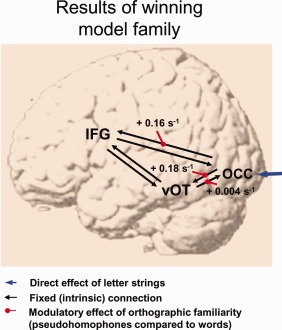
Connectivity changes for pseudohomophones compared to words. Average values of the winning model family. Connectivity values correspond to rate constants, and are given in s−1 (hertz). For example, if effective connectivity from area A to area B is + 0.10 s−1, this means that, per unit time, the increase in activity in B corresponds to 10% of the activity in A (den Ouden, 2009). [Color figure can be viewed in the online issue, which is available at http://wileyonlinelibrary.com]
Table 2.
Average connectivity parameters (s−1) for the winning model family
| Connection | Parameter estimates (s−1) | t(18) | |||
|---|---|---|---|---|---|
| From | To | M | SEM | ||
| Intrinsic connectivity | OCC | OT | 0.088 | 0.024 | 3.6a |
| OCC | IFG | 0.047 | 0.035 | 1.3 | |
| OT | OCC | 0.051 | 0.014 | 3.5a | |
| OT | IFG | 0.121 | 0.054 | 2.2 | |
| IFG | OT | 0.128 | 0.056 | 2.3 | |
| IFG | OCC | 0.046 | 0.013 | 3.5a | |
| Modulatory effect of orthographic familiarity | OCC | OT | 0.181 | 0.034 | 5.3b |
| OCC | IFG | 0.158 | 0.037 | 4.3b | |
| OT | OCC | 0.004 | 0.001 | 2.9c | |
| OT | IFG | 0.017 | 0.007 | 2.5 | |
| IFG | OT | 0.009 | 0.004 | 2.5 | |
| IFG | OCC | 0.005 | 0.002 | 2.8 | |
| On region | |||||
| Direct effect of letter strings | OCC | 0.093 | 0.012 | 7.5b | |
P < 0.05, corrected.
P < 0.01, corrected.
P < 0.01, uncorrected.
For each parameter, we tested whether it differed significantly from zero across subjects. Note that in DCM, connectivity parameters are estimated using priors with zero mean (so‐called shrinkage priors), so—in the absence of neuronal activation—estimates of the coupling parameters shrink toward zero. Results were Bonferroni‐corrected for the number of comparisons, i.e., the number of parameters for each class. Results in Table 2 show strong and reliable bidirectional intrinsic connectivity between the occipital cortex and the left vOT. In absolute terms, forward connectivity was stronger compared to the backward connectivity on this pathway. In addition, we found significant fixed connectivity on the pathway from the left inferior frontal gyrus to the occipital cortex. Fixed connectivity between the left vOT and the left inferior frontal gyrus was high in absolute values. Because of high variance, fixed connectivity on this pathway did not survive our correction for multiple comparisons.
Table 2 also reports parameter estimates of modulatory effects of orthographic familiarity on connection strength. Reliable modulatory effects of orthographic familiarity were found on the forward pathways from the occipital cortex to the left vOT (+ 0.18 s−1) and from the occipital cortex to the left inferior frontal gyrus (+ 0.16 s−1). We also note that we observed a modulation (+ 0.004 s−1) of the backward path from the left vOT to the occipital cortex. This effect did just not reach significance after correcting for multiple comparisons (P = 0.009), but is highly significant when uncorrected. In sum, results mainly show that effective brain connectivities from the occipital cortex to the left vOT and from the occipital cortex to the left inferior frontal gyrus massively increase (more than doubled to compared to the fixed connectivities) for pseudohomophones compared to words.
DISCUSSION
The present study followed‐up the finding of higher activation for pseudohomophones compared to words in the left vOT [see Borowsky et al., 2006; Bruno et al., 2008; Kronbichler et al., 2007, 2009; van der Mark et al., 2009; Twomey et al., 2011]. We relied on DCM [Friston et al., 2003] to explain this finding in terms of bottom‐up versus top‐down influences on the left vOT. We analyzed effective connectivity within a three‐area network comprising an area in the occipital cortex, the left vOT, and the left inferior frontal gyrus. We observed that bottom‐up signaling from the occipital cortex to the left vOT strongly increased for pseudohomophones. In addition, a comparatively small increase in top‐down connectivity form the left vOT to the occipital cortex was found. In contrast, signaling between the left inferior frontal gyrus and the left vOT did not differ between words and pseudohomophones.
Top‐Down and Bottom‐Up Connectivity of the Left vOT
The main question of our study focused on the modulatory effects obtained with our analysis. We were interested in how top‐down and/or bottom‐up signaling to the left vOT changes for pseudohomophones compared to words. Results from our analysis show that top‐down signaling from the left inferior frontal gyrus does not change for pseudohomophones. Put differently, the activation difference between pseudohomophones and words in the left vOT is not driven by a change in top‐down influences. This finding fits to our expectation that pseudohomophones and words engage the same (or similar) higher level representations. In our phonological lexical decision task (Does the item sound like a word?) pseudohomophones and words corresponded to the same phonological words—which were associated with the same meanings. Moreover, words and pseudohomophones received the same responses (yes, it does sound like a word). If the same higher level representations are engaged, the same top‐down signals can be expected. This prediction is supported by our data.
Another main finding of the present study was the observation of a strong increase in signaling on the bottom‐up connection from occipital cortex to the left vOT for pseudohomophones (compared to words). This finding can be linked to the functional explanation of left vOT activation differences proposed by Kronbichler et al. [2007]. Occipital activations for the visual inputs of words and pseudohomophones are propagated along the ventral visual stream. For words, the propagated signals converge onto a matching orthographic representation, e.g., taxi [see also Dehaene and Cohen, 2011; Glezer et al., 2009]. In the case of pseudohomophones, the propagated signals from occipital cortex do not converge, but (partially) activate multiple orthographic representations in the left vOT. For example, the letter sequence t‐a‐k‐s‐i may activate the orthographic representations take, table, taxi, sit, sister and so on.
In addition to the observed increase in bottom‐up signaling, our results also show a slight increase in top‐down signaling from the left vOT to the occipital cortex. Although this finding just not survived a correction for multiple comparisons, it is an interesting trend worth discussing. For example, it relates to the propositions formulated in the “Interactive Account” of functional specialization, which was recently proposed by Price and Devlin [2011]. “The Interactive Account is based on the premise that perception involves recurrent or reciprocal interactions between sensory cortices and higher order processing regions via a hierarchy of forward and backward connections.” [Price and Devlin, 2011, p. 247]. Interactions are reciprocal, because in addition to bottom‐up signaling of sensory input, higher order processing regions send top‐down predictions. These are based on prior experience with a stimulus and subserve the resolution of uncertainty about the sensory input. If a stimulus (e.g., a pseudohomophone) is potentially meaningful, it will engage high‐level representations. However, different from regular words, the top‐down predictions from higher levels cannot efficiently predict the low‐level visual representation, resulting in more prediction error, and thus, higher activation. Based on the assumption that the left vOT contains neurons tuned to complex orthographic features such as morphemes or whole‐words [Dehaene and Cohen, 2011; Glezer et al., 2009; Kronbichler et al., 2007]—we interpret the left vOT as having “higher order” processing properties itself. From this perspective, the pattern of top‐down connectivity from the occipitotemporal cortex to the occipital cortex fits nicely to what was proposed by Price and Devlin [2011]. The (partially) activated orthographic representations for taksi (e.g., take, table, taxi, sit, sister) cannot efficiently predict the letter sequence t‐a‐k‐s‐i, thus leading to increased top‐down prediction error.
Other Interactions
Besides the interactions of the left vOT, the present analysis found that bottom‐up signaling from the occipital cortex to the left inferior frontal gyurs increases for pseudohomophones compared to words. This finding may reflect a dorsal visual processing pathway, which connects occipital areas via the parietal cortex to frontal areas. Such pathway was linked to sublexical reading processes [Cohen et al., 2008; Levy et al., 2009; Richlan et al., 2010]. Alternatively, it could reflect a pathway involving the superior temporal sulcus, which was recently highlighted in Seghier et al. [2012; see also Richardson et al., 2011]. The present study is limited in its potential to characterize this finding, as our network model included no areas of the dorsal visual pathway. However, our interpretation that pseudohomophones are not efficiently processed by orthographic feature detectors in the left vOT calls for an additional processing mechanism which enables their reading. For example, Cohen et al. [2008] proposed that whenever the left vOT fails to efficiently process a word in parallel, dorsal parietal areas will be engaged. Parietal areas deploy a serial reading strategy by guiding attention toward sublexical features of a string, for example, single letters. Our finding of increased signaling from the occipital cortex to the left inferior frontal gyrus may reflect such serial sublexical processing.
Limitations
We focused our DCM analysis on the question how bottom‐up versus top‐down influences are driving activation for pseudohomophones (relative to words) in the left vOT. We constructed the simplest model for this question, consisting of three brain areas: One low‐level visual area in the occipital cortex, one area in the left vOT, and one higher level language area in the left inferior frontal gyrus. However, we do not suggest that our three‐area network model is a comprehensive model of visual word processing. Such a model would likely include multiple additional frontal, temporal, and parietal areas, as well as areas of the right hemisphere. Adding more regions into a DCM makes a systematic model comparison more costly. For example, our three‐area network had 64 different model variants. A five‐area network (for our experiment) would have 1024 possible model variants; a seven‐area network would have 16.384 model variants, and so on. It is important to note, however, that leaving out areas from a model does not reduce the theoretical interest of results [Mechelli et al., 2007]. For example, our analysis shows that the occipital cortex is functionally coupled to the left vOT. A number of relevant ventral stream processing areas are lying in‐between the occipital cortex and the left vOT. It is plausible that, in our task, signals from the occipital cortex were processed in other ventral stream areas before they reached the left vOT. However, this will not change the findings that (i) the occipital cortex and the left vOT are functionally associated during visual word recognition and (ii) that this functional association becomes stronger when an orthographically unfamiliar letter‐string is processed. Another limitation must be noted with respect to our finding of absent of top‐down modulations from the IFG. The present analysis only looked at top‐down signaling from the posterior aspect of the IFG (pars opercularis), which is associated with phonological segmentation [e.g., Jobard et al., 2003]. We cannot rule out the possibility of top‐down modulation on vOT from other regions that show greater activation for pseudohomophones and were not included in our model, for example, areas associated with lexical selection such as the IFG pars triangularis.
CONCLUSIONS
We used DCM for fMRI to analyze how top‐down and bottom‐up neural signalling to the left vOT changes for processing of pseudohomophones compared to processing of words. We observed that bottom‐up signaling from the occipital cortex to the left vOT strongly increases for pseudohomophones. In contrast, top‐down signaling from the left inferior frontal gyrus to the left vOT did not differ between words and pseudohomophones. Since we were interested in the functional role of bottom up signals, we selected an experimental task which—in our understanding—is optimized to detect differences in bottom‐up rather than top‐down signaling. The contrast between pseudohomophones and words is a special case where unfamiliar letter strings engage the same phonological and semantic representations as regular words. We want to emphasize that the present DCM findings therefore do not imply irrelevance of top‐down signals for the functioning of the left vOT in general. There is overwhelming evidence that in many cases of letter‐string and visual object processing, top‐down signaling is crucial for the left vOTs functional response [e.g., Devlin et al., 2006; Hellyer et al., 2011; Kherif et al., 2011; Mano et al., 2012; Reich et al., 2011; Twomey et al., 2011]. Still, the present study shows that bottom‐up signaling is of theoretical importance for understanding the function of this area. Our results can be explained by models that assume that the left vOT hosts neurons that are tuned to complex orthographic features [e.g., Dehaene and Cohen, 2011; Kronbichler et al., 2007]: Bottom‐up signals converge onto a matching orthographic representation in the case of words. In the case of pseudohomophones, however, they do not converge on a specific orthographic representation, but instead partially activate multiple representations, reflected in increased effective connectivity.
Supporting information
Supporting Information Table 1.
Supporting Information Table 2.
ACKNOWLEDGMENTS
The authors thank the anonymous reviewers for their excellent comments. MS wants to thank Benjamin Gagl for a helpful discussion about an earlier version of this manuscript.
REFERENCES
- Baayen RH, Piepenbrock R, van Rijn H (1993):The CELEX Lexical Database (CD‐ROM). Philadelphia, PA:Linguistic Data Consortium, University of Pennsylvania. [Google Scholar]
- Bitan T, Booth JR, Choy J, Burman DD, Gitelman DR, Mesulam MM (2005): Shifts of effective connectivity within a language network during rhyming and spelling. J Neurosci 25:5397–5403. [DOI] [PMC free article] [PubMed] [Google Scholar]
- Bitan T, Burman DD, Lu D, Cone NE, Gitelman DR, Mesulam MM, Booth JR (2006): Weaker top‐down modulation from the left inferior frontal gyrus in children. NeuroImage 33:991–998. [DOI] [PMC free article] [PubMed] [Google Scholar]
- Bitan T, Cheon J, Lu D, Burman DD, Gitelman DR, Mesulam MM, Booth JR (2007): Developmental changes in activation and connectivity in phonological processing. NeuroImage 38:564–575. [DOI] [PMC free article] [PubMed] [Google Scholar]
- Bitan T, Cheon J, Lu D, Burman DD, Booth JR (2009): Developmental increase in top‐down and bottom‐up processing in a phonological task: An effective connectivity, fMRI study. J Cogn Neurosci 21:1–11. [DOI] [PMC free article] [PubMed] [Google Scholar]
- Bolger DJ, Perfetti CA, Schneider W (2005): Cross‐cultural effect on the brain revisited: Universal structures plus writing system variation. Hum Brain Mapp 25:92–104. [DOI] [PMC free article] [PubMed] [Google Scholar]
- Booth JR, Mehdiratta N, Burman DD Bitan T (2008): Developmental increases in effective connectivity to brain regions involved in phonological processing during tasks with orthographic demands. Brain Res 1189:78–89. [DOI] [PMC free article] [PubMed] [Google Scholar]
- Borowsky R, Cummine J, Owen WJ, Friesen CK, Shih F, Sarty GE (2006): FMRI of ventral and dorsal processing streams in basic reading processes: Insular sensitivity to phonology. Brain Topogr 18:233–239. [DOI] [PubMed] [Google Scholar]
- Bruno JL, Zumberge A, Manis F, Lu Z, Goldman JG (2008): Sensitivity to orthographic familiarity in the occipito‐temporal region. NeuroImage 39:1988–2001. [DOI] [PMC free article] [PubMed] [Google Scholar]
- Cao F, Bitan T Booth JR (2008): Effective brain connectivity in children with reading difficulties during phonological processing. Brain Lang, 107:91–101. [DOI] [PMC free article] [PubMed] [Google Scholar]
- Cohen L, Dehaene S, Naccache L, Lehéricy S, Dehaene‐Lambertz G, Hénaff M, et al. (2000): The visual word form area. Spatial and temporal characterization of an initial stage of reading in normal subjects and posterior split‐brain patients. Brain 123:291–307. [DOI] [PubMed] [Google Scholar]
- Cohen L, Martinaud O, Lemer C, Lehéricy S, Samson Y, et al. (2003): Visual word recognition in the left and right hemispheres: Anatomical and functional correlates of peripheral alexias. Cereb Cortex 13:1313–1333 [DOI] [PubMed] [Google Scholar]
- Cohen L, Dehaene S, Vinckier F, Jobert A, Montavont A (2008): Reading normal and degraded words: Contribution of the dorsal and ventral visual pathways. NeuroImage 40:353–366. [DOI] [PubMed] [Google Scholar]
- Dehaene S, Cohen L, Sigman M, Vinckier F (2005): The neural code for written words: A proposal. Trends Cogn Sci 9:335–341. [DOI] [PubMed] [Google Scholar]
- Dehaene S, Cohen L (2011): The unique role of the visual word form area in reading. Trends Cogn Sci 15:254–262. [DOI] [PubMed] [Google Scholar]
- den bOuden H (2009):Dynamic Causal Modeling: Theory. SPM Course; October 22–24th, London, UK: Available at: http://www.fil.ion.ucl.ac.uk/spm/course/slides09-oct/09_DCM_fMRI.ppt [Google Scholar]
- Devlin JT, Jamison HL, Gonnerman LM, Matthews PM (2006): The role of the left posterior fusiform gyrus in reading. J Cogn Neurosci 18:911–922. [DOI] [PMC free article] [PubMed] [Google Scholar]
- Friston KJ, Glaser DE, Henson RNA, Kiebel S, Phillips C, Ashburner J (2002): Classical and Bayesian inference in neuroimaging: Applications. NeuroImage 16:484–512. [DOI] [PubMed] [Google Scholar]
- Friston KJ, Harrison L, Penny W (2003): Dynamic causal modeling. NeuroImage 19:1273–302 [DOI] [PubMed] [Google Scholar]
- Friston KJ, Mattout J, Trujillo‐Barreto N, Ashburner J, Penny W (2007): Variational free energy and the Laplace approximation. NeuroImage 34:220–234. [DOI] [PubMed] [Google Scholar]
- Gaillard R, Naccache L, Pinel P, Clemenceau S, Volle E, Hasboun D, et al. (2006): Direct intracranial, fMRI, and lesion evidence for the causal role of left inferotemporal cortex in reading. Neuron 50:191–204. [DOI] [PubMed] [Google Scholar]
- Genovese CR, Lazar NA, Nichols T (2002): Thresholding of statistical maps in functional neuroimaging using the false discovery rate. NeuroImage 15:870–878. [DOI] [PubMed] [Google Scholar]
- Glezer LS, Jiang X, Riesenhuber M (2009): Evidence for highly selective neuronal tuning to whole words in the “visual word form area”. Neuron 62:199–204. [DOI] [PMC free article] [PubMed] [Google Scholar]
- Heim S, Eickhoff SB, Ischebeck AK, Friederici AD, Stephan KE, Amunts K (2009): Effective connectivity of the left BA 44 BA 45 and inferior temporal gyrus during lexical and phonological decisions identified with DCM. Hum Brain Mapp 30:392–402. [DOI] [PMC free article] [PubMed] [Google Scholar]
- Hellyer PJ, Woddhead ZVJ, Leech R, Wise RJS (2011): An investigation of Twenty/20 vision in reading. J Neurosci 31:14631–14638. [DOI] [PMC free article] [PubMed] [Google Scholar]
- Henson RNA (2004): Analysis of fMRI time series: linear time‐invariant models, event‐related fMRI and optimal experimental design In Frackowiak RSJ, Friston KJ, Frith C, Dolan R, Price CJ, Zeki S, et al. Eds.,Human brain function 2nd ed., pp.793–822. London:Academic Press. [Google Scholar]
- Jobard G, Crivello F, Tzourio‐Mazoyer N (2003): Evaluation of the dual route theory of reading: A meta‐analysis of 35 neuroimaging studies. NeuroImage 20:693–712. [DOI] [PubMed] [Google Scholar]
- Kass RE, Raftery AE (1995): Bayes factors. J Am Stat Assoc 90:773–795. [Google Scholar]
- Kherif F, Josse G, Price CJ (2011): Automatic top‐down processing explains common left‐occipito‐temporal responses to visual words and objects. Cereb Cortex 21:103–114. [DOI] [PMC free article] [PubMed] [Google Scholar]
- Kronbichler M, Bergmann J, Hutzler F, Staffen W, Mair A, Ladurner G, et al. (2007): Taxi vs. Taksi: Orthographic word recognition in the left ventral occipitotemporal cortex. J Cogn Neurosci 19:1584–1594. [DOI] [PMC free article] [PubMed] [Google Scholar]
- Kronbichler M, Klackl J, Richlan F, Schurz M, Staffen W, Ladurner G, et al. (2009): On the functional neuroanatomy of visual word processing: effects of case and letter deviance. J Cogn Neurosci 211:1–8. [DOI] [PMC free article] [PubMed] [Google Scholar]
- Levy J, Pernet C, Treserras S, Boulanouar K, Aubry F, Demonet JF, Celsis P (2009): Testing for the dual‐route cascade model in the brain: An fMRI effective connectivity account of an efficient reading style. PloS One 4:E6675.rr [DOI] [PMC free article] [PubMed] [Google Scholar]
- Mano QR, Humphries C, Desai RH, Seidenberg MS, Osmon DC, Stengel BC Binder JR (2012): The role of the left occipitotemporal cortex in reading: Reconciling stimulus, task, and lexicality effects. Cereb Cortex, doi: 10.1093/cercor/bhs093. [DOI] [PMC free article] [PubMed] [Google Scholar]
- Mechelli A, Allen P, Edson A, Fu CHY, Williams SCR, Brammer MJ, Johns LC, McGuire PK (2007): Misattribution of speech and impaired connectivity in patients with auditory verbal hallucinations. Hum Brain Mapp 28:1213–1222. [DOI] [PMC free article] [PubMed] [Google Scholar]
- Mechelli A, Crinion JT, Long S, Lambon‐Ralph MA, Patterson K, McClelland JL, Price CJ (2005): Dissociating reading processes on the basis of neuronal interactions. J Cogn Neurosci 17:1753–1765. [DOI] [PubMed] [Google Scholar]
- Nakamura K, Dehaene S, Jobert A, Le Bihan D, Kouider S (2007): Task‐specific change of unconscious neural priming in the cerebral language network. Proc Natl Acad Sci 104:19643–19648. [DOI] [PMC free article] [PubMed] [Google Scholar]
- Penny WD, Stephan KE, Daunizeau J, Rosa MJ, Friston KJ, Schofield TM, Leff AP (2010): Comparing families of dynamic causal models. PLoS Comput Biol 6:E1000709. [DOI] [PMC free article] [PubMed] [Google Scholar]
- Price CJ, Devlin JT (2003): The myth of the visual word form area. NeuroImage 19:473–481. [DOI] [PubMed] [Google Scholar]
- Price CJ Devlin JT (2011): The interactive account of ventral occipitotemporal contributions to reading. Trends Cogn Sci 15:246–253. [DOI] [PMC free article] [PubMed] [Google Scholar]
- Reich L, Szwed L, Cohen L, Amedi A (2011): A ventral visual stream reading center independent of visual experience. Neuron 21:363–368. [DOI] [PubMed] [Google Scholar]
- Richlan F, Sturm D, Schurz M, Kronbichler M, Ladurner G, Wimmer H (2010): A common left occipito‐temporal dysfunction in developmental dyslexia and acquired letter‐by‐letter reading? PLoS One 5:e12073. [DOI] [PMC free article] [PubMed] [Google Scholar]
- Roberts DJ, Woollams AM, Kim E, Beeson PM, Rapcsak SZ, Lambon Ralph MA: Efficient visual object and word recognition relies on high spatial frequency coding in the left posterior fusiform gyrus: Evidence from a case‐series of patients with ventral occipito‐temporal cortex damage. Cereb. Cortex first published online August 24, 2012. doi: 10.1093/cercor/bhs224. [DOI] [PMC free article] [PubMed]
- Richardson FM, Seghier ML, Leff AP, Thomas MSC, Price CJ (2011): Multiple routes from occipital to temporal cortices during reading. J Neurosci 31:8239–8247. [DOI] [PMC free article] [PubMed] [Google Scholar]
- Seghier ML, Price CJ (2010): Reading aloud boosts connectivity through the putamen. Cereb Cortex 20:570–582. [DOI] [PMC free article] [PubMed] [Google Scholar]
- Seghier ML, Neufeld NH, Zeidman P, Leff AP, Mechelli A, Nagendran A, Riddoch JM, Humphreys GW, Price CJ: Reading without the left ventral occipito‐temporal cortex. Neuropsychologia 50:3621–3635. [DOI] [PMC free article] [PubMed] [Google Scholar]
- Sonty SP, Mesulam MM, Weintraub S, Johnson NA, Parrish TB, Gitelman DR (2007): Altered effective connectivity within the language network in primary progressive aphasia. J Neurosci 27:1334–1345. [DOI] [PMC free article] [PubMed] [Google Scholar]
- Stephan KE, Penny WD, Daunizeau J, Moran R, Friston KJ (2010): Bayesian model selection for group studies. NeuroImage 46:1004–1017. [DOI] [PMC free article] [PubMed] [Google Scholar]
- Twomey T, Kawabata Duncan KJ, Price CJ, Devlin JT (2011): Top‐down modulation of ventral occipito‐temporal responses during visual word recognition. NeuroImage 55:1242–51 [DOI] [PMC free article] [PubMed] [Google Scholar]
- van der Mark S, Bucher K, Maurer U, Schulz E, Brem S, Buckelmüller J, Kronbichler M, Loenneker T, Klaver P, Martin E, Brandeis D (2009): Children with dyslexia lack multiple specializations along the visual word‐form (VWF) system. NeuroImage 47:1940–1949. [DOI] [PubMed] [Google Scholar]
- Wager TD, Nichols TE (2003): Optimization of experimental design in fMRI: a general framework using a genetic algorithm. NeuroImage 18:293–309. [DOI] [PubMed] [Google Scholar]
Associated Data
This section collects any data citations, data availability statements, or supplementary materials included in this article.
Supplementary Materials
Supporting Information Table 1.
Supporting Information Table 2.