Disruption of structural and functional networks in long‐standing multiple sclerosis

Abstract

Both gray matter atrophy and disruption of functional networks are important predictors for physical disability and cognitive impairment in multiple sclerosis (MS), yet their relationship is poorly understood. Graph theory provides a modality invariant framework to analyze patterns of gray matter morphology and functional coactivation. We investigated, how gray matter and functional networks were affected within the same MS sample and examined their interrelationship. Magnetic resonance imaging and magnetoencephalography (MEG) were performed in 102 MS patients and 42 healthy controls. Gray matter networks were computed at the group‐level based on cortical thickness correlations between 78 regions across subjects. MEG functional networks were computed at the subject level based on the phase‐lag index between time‐series of regions in source‐space. In MS patients, we found a more regular network organization for structural covariance networks and for functional networks in the theta band, whereas we found a more random network organization for functional networks in the alpha2 band. Correlation analysis revealed a positive association between covariation in thickness and functional connectivity in especially the theta band in MS patients, and these results could not be explained by simple regional gray matter thickness measurements. This study is a first multimodal graph analysis in a sample of MS patients, and our results suggest that a disruption of gray matter network topology is important to understand alterations in functional connectivity in MS as regional gray matter fails to take into account the inherent connectivity structure of the brain. Hum Brain Mapp 35:5946–5961, 2014. © 2014 Wiley Periodicals, Inc.

INTRODUCTION

Multiple sclerosis (MS) is a chronic inflammatory and neurodegenerative disease of the central nervous system, often leading to a wide spectrum of clinical symptoms such as physical disability and cognitive impairment. Although the disease was initially recognized as merely a demyelinating disease, the discrepancy between classical magnetic resonance imaging (MRI) findings such as white matter lesion load and clinical dysfunction led to a search for alternative pathological substrates for clinical dysfunction [Geurts and Barkhof, 2008]. In this context, both gray matter atrophy and changes in neuronal activity have been reported and linked to physical disability and cognitive impairment in MS [Calabrese et al., 2007, 2010; Geurts and Barkhof, 2008; Hardmeier et al., 2012; Steenwijk et al., 2014; Tewarie et al., 2013a]. Bridging the gap between gray matter atrophy and changes in neuronal activity may be crucial for understanding disease mechanisms that eventually lead to clinical symptoms. However, the relationship between changes in gray matter and disrupted activation patterns is still unclear, and this is probably due to the fact that localized measurements fail to fully take into account the inherent connectivity structure of the brain.

Graph theory provides a framework to study brain connectivity changes in MS by representing the brain as a complex network [Stam and van Straaten, 2012]. Such a network consists of a set of brain regions (nodes) interconnected with links. Links can be measured based on the communication between distinct brain regions (i.e., functional connectivity); based on physical connections between these brain regions (e.g., as measured by diffusion tensor imaging) and based on covariance of gray matter properties of these regions (i.e., structural connectivity), such as cortical thickness [Alexander‐Bloch et al., 2013a]. These three types of brain connectivity robustly show a nonrandom organization that is characterized by dense local connectivity and relatively sparse long‐range connections. Such a topology has been associated with a balance of integration and segregation, and a minimization of economical costs and maximization of efficiency [Bullmore and Sporns, 2009; Rubinov and Sporns, 2010].

Previous studies have investigated either structural covariance or functional network organization in MS [Gamboa et al., 2014; Hardmeier et al., 2012; He et al., 2009; Schoonheim et al., 2011; Tewarie et al., 2013b]. Structural covariance networks showed disrupted integration in MS, which was proportional to white matter lesion load [He et al., 2009]. Functional network studies have revealed lower integration in functional networks in MS as obtained with functional magnetic resonance imaging (fMRI) and magnetoencephalography (MEG) [Gamboa et al., 2014; Hardmeier et al., 2012; Louapre et al., 2014; Schoonheim et al., 2011]. However, it is still unknown how alterations of structural covariance and functional networks in MS are related to each other. One of the hypotheses is that brain regions that show functional coactivation tend to covary in thickness (Alexander‐Bloch et al., 2013). Therefore, disruption of structural covariance or functional networks may influence each other. However, methodological hurdles such as differences in connectivity density impede direct comparison of networks of different studies and modalities [Fornito et al., 2013; van Wijk et al., 2010]. The minimum spanning tree (MST; a subnetwork containing the strongest connections, see Methods for more details), is a promising approach that enables comparison of networks. We recently showed that in comparison to healthy controls the MSTs of MS patients are characterized by lower integration of information and loss of hierarchical structure of functional networks, and that this was related to a decline in cognitive performance [Tewarie et al., 2013b]. It is still unclear how these MST changes relate to other, more frequently used, graph theoretical measures.

The aim of the present study is to investigate how changes in gray matter atrophy relate to disruption of functional networks, as clarifying this relationship could give more insight in disease mechanisms in MS. To this end, we investigate how structural covariance networks (based on cortical thickness correlations) and MEG functional networks were affected by the disease within the same MS sample. We further investigated the relationship between structural covariance and functional networks as we hypothesized that disruption of functional networks may co‐occur with disruption of structural covariance networks. In addition, we analyzed if this relationship could merely be explained by an association between regional gray matter thickness and functional network connectivity. We obtained structural covariances at the group level and MEG functional networks at the subject level. For all networks, we computed conventional graph theoretical measures to increase the interpretability of our results within the context of previous studies. Finally, we investigated MST measures, since these minimize potential biases that might arise as a consequence of constructing networks for different imaging modalities.

METHODS

Participants

In total, 120 MS patients and 44 healthy controls were recorded. Data from some subjects were excluded from analyses because of neurological comorbidity (N = 10), too many artifacts or noise in the raw MEG data (N = 2), or absence of MRI or MEG data (N = 8). Consequently, 102 MS patients and 42 controls remained in the study. Patients were recruited from the MS database at the VUmc MS center and were part of a long disease duration cohort. The study protocol was approved by the Local Research Ethics Committee (Medical Ethical Review Committee of VU University Medical Center), whose ethics review criteria conformed to the Helsinki declaration. All subjects gave written informed consent prior to participation. An overview of the applied methods is depicted in Figure 1.

Figure 1.

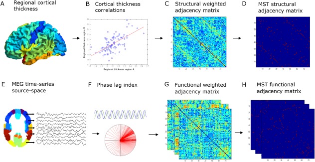
Overview of the applied methods: (A) regional cortical thickness was estimated by computing the distance between the surfaces of the pial and white matter layers as obtained from T1‐weighted structural images. We then used the AAL atlas (78 cortical areas) to obtain an average cortical thickness value across the vertices within a region of interest (ROI). (B) Cortical thickness correlations between all possible pair of regions were subsequently computed across subjects to obtain a structural adjacency matrix at the group level (C). From this, (D) the minimum spanning tree (MST), an unique acyclic subnetwork, was obtained. (E) MEG time‐series were projected with a beamformer approach onto the same AAL atlas parcellation. (F) The phase lag index (PLI) was computed as a measure of functional connectivity between regions to obtain a frequency‐dependent functional adjacency matrix (G). Subsequently, the MST was computed (H). For both structural and functional data, the weighted adjacency matrices were normalized (by dividing each link weight by the mean link weight of that adjacency matrix) to minimize biases due to differences in average connectivity. Network measures were computed for the complete weighted networks and for the MSTs. [Color figure can be viewed in the online issue, which is available at http://wileyonlinelibrary.com.]

Data Acquisition

MR imaging of the brain was performed on a 3.0T whole body scanner (GE Signa HDxt, Milwaukee, WI) using an eight‐channel phased array headcoil. The protocol included, a three‐dimensional T1‐weighted fast spoiled gradient echo sequence (repetition time [TR] 7.8 ms, echo time [TE] 3 ms, inversion time [TI] 450 ms, 12° flip angle [FA], sagittal 1.0‐mm‐thick slices, 0.94 × 0.94 mm² in‐plane resolution) for cortical segmentation, and a three‐dimensional fluid attenuated inversion recovery image (FLAIR; TR 8,000 ms, TE 125 ms, TI 2,350 ms, sagittal 1.2‐mm‐thick slices, 0.98 × 0.98 mm² in‐plane resolution) for lesion detection.

MEG data were recorded using a 306‐channel whole‐head MEG system (Elekta Neuromag, Oy, Helsinki, Finland) while participants were in a supine position in a magnetically shielded room (Vacuumschmelze, Hanau, Germany). Fluctuations in magnetic field strength were recorded during a no‐task, eyes‐open condition for 3 min (not analyzed here) and eyes‐closed condition for five consecutive minutes with a sample frequency of 1,250 Hz. An antialiasing filter of 410 Hz and a high‐pass filter of 0.1 Hz were applied online and other artifacts were removed offline using the temporal extension of Signal Space Separation (tSSS) in MaxFilter software with a sliding window of 10 s (Elekta Neuromag Oy, version 2.2.10) [Taulu and Simola, 2006; Taulu and Hari, 2009]. Channels that were malfunctioning during the recording, for example, due to excessive noise, were identified by automatic and visual inspection of the data and removed before applying tSSS. The number of excluded channels varied between 1 and 12 and did not differ between MS patients and healthy controls (Mann–Whitney P > 0.05). The tSSS filter was then used to remove noise signals that SSS without temporal extension failed to discard, typically from noise sources near the head, using a subspace correlation limit of 0.9. The head position relative to the MEG sensors was recorded continuously using the signals from four head‐localization coils. The head‐localization coil positions were digitized, as well as the outline of the participants scalp (∼500 points), using a 3D digitizer (3SpaceFastTrack, Polhemus, Colchester, VT). Scalp surfaces of all subjects were coregistered to their structural MRIs using a surface‐matching procedure, with an estimated resulting accuracy of 4 mm [Whalen et al., 2008]. A single best fitting sphere was fitted to the outline of the scalp as obtained from the coregistered MRI, which was used as a volume conductor model for the beamformer approach described below.

Estimation of Structural Covariance

Cortical thickness was measured with FreeSurfer 5.1 software after lesion filling in MS (see Supporting Information for lesion filling technique) [Dale et al., 1999; Fischl et al., 1999]. In short, FreeSurfer determines the pial and white matter surface of the cortex based on a T1‐weighted structural image. The distance between these surfaces gives the vertexwise cortical thickness (i.e., the perpendicular thickness at each location) of the cortex. All cortical segmentations were visually inspected for gross errors, which were manually corrected and rerun when necessary.

Subsequently, a surface‐based version of the automated anatomical labeling (AAL) atlas was constructed to parcellate 78 identical areas for the cortical thickness and the MEG network analysis [Gong et al., 2009]. To this end, the T1‐weighted image of each healthy control was nonlinearly registered to montreal neurological institute (MNI)‐space using FMRIB's linear image registration tool (FLIRT) and FSL's nonlinear image registration tool (FNIRT) (part of FSL 5.0.2; http://fsl.fmrib.ox.ac.uk/). The AAL atlas was warped to subject space using the inverse transformation of MNI registration, to obtain a subject‐specific AAL parcellation. Each subject‐specific volumetric atlas was subsequently sampled on the surface halfway the gray matter and white matter, resulting in a rough AAL‐parcellation containing 39 cortical areas per hemisphere for each subject. These were subsequently used to train FreeSurfer's probabilistic cortical surface classifier that makes use of the folding pattern and curvature of the surface to label cortical regions [Desikan et al., 2006]. By training the classifier with a large sample of ‘less‐perfect' examples, ‘smooth’ AAL‐parcellations could be obtained that are suitable for regional cortical thickness analysis. Cortical thickness was averaged across the vertices in each AAL region, resulting in 78 measures of cortical thickness per subject. Effects of age, gender, age‐gender interaction and mean overall cortical thickness were removed with linear regression analyses and the resulting residuals were used for subsequent analyses [He et al., 2007].

Cortical thickness correlations were computed with Pearson correlations of average adjusted cortical thickness between AAL areas across subjects for the MS patients and healthy controls separately, resulting in two unthresholded (78 × 78) cortical thickness correlation matrices. Then, we applied a transformation of the raw correlation matrix: a value of one was added to all elements in the matrix and the result was subsequently divided by two. This transformation was performed to ensure that all matrix elements were positive since most algorithms that we used to compute topological measures require positive weights. Last, for descriptive purposes we also estimated white matter lesion load and whole brain atrophy using kNN‐TTP and SIENAX (part of FSL 5.0.2; http://fsl.fmrib.ox.ac.uk/) (see Supporting Information).

Estimation of MEG Functional Connectivity

A beamformer approach was adopted to map MEG data from sensor level to source space [Hillebrand et al., 2012]. First, the coregistered MRI was spatially normalized to a template MRI using the SEG‐toolbox in SPM8 [Friston et al., 2004; Ashburner and Friston, 2005; Weiskopf et al., 2011]. The AAL atlas was used to label the voxels in a subject's normalized coregistered MRI [Tzourio‐Mazoyer et al., 2002]. Subcortical structures were removed, and the voxels in the remaining 78 cortical regions of interest (ROIs) were used for further analysis [Gong et al., 2009], after inverse transformation to the patient's coregistered MRI. Next, neuronal activity in the labeled voxels was reconstructed using a scalar beamformer implementation (Elekta Neuromag Oy, beamformer, version 2.1.27) similar to Synthetic Aperture Magnetometry [Robinson and Vrba, 1999].

Briefly, this beamformer sequentially reconstructs the activity for each voxel in a predefined grid covering the entire brain (spacing 2 mm) by selectively weighting the contribution from each MEG sensor to a voxel's time‐series. The beamformer weights are based on the data (recorded time‐series) covariance matrix and the forward solution (lead field) of a dipolar source at the voxel location A time‐window of, on average, 323 s (range 181–476 s; range MS patients 192–476 s; range healthy controls 181–349, Mann–Whitney test, P > 0.05) was used to compute the data covariance matrix. Singular value truncation was used when inverting the data covariance matrix, using a default setting of 1 × 10⁻⁶ for the ratio between the largest and smallest acceptable singular value. For each voxel in our predefined grid the pseudo‐Z values, using a unity matrix as estimate for the noise covariance matrix [Hillebrand and Barnes, 2005], were computed for different frequency bands (delta [0.5–4 Hz], theta [4–8 Hz], lower alpha [8–10 Hz], upper alpha [10–13 Hz], beta [13–30 Hz], and lower gamma [30–48 Hz]). Each ROI in the atlas contains many voxels, and the number of voxels per ROI differs. To obtain a representation of a ROI by its time‐series, we selected, for each ROI and frequency band separately, the voxel with maximum pseudo‐Z value in that frequency band. For this peak‐voxel, we projected the broadband (0.5–48 Hz) time‐series though the broadband beamformer weights to obtain a time‐series for a ROI (six time‐series in total, i.e., one for each frequency band). Subsequently, the obtained time‐series were downsampled four times. Just as in previous studies, for each subject, for each frequency band, the same five artifact free epochs of 4,096 samples (13.1072 s) were selected (PT) to obtain stable results, using BrainWave software (version 0.9.101; http://home.kpn.nl/stam7883/brainwave.html) [de Haan et al., 2012; Douw et al., 2013; Hardmeier et al., 2012; Schoonheim et al., 2011; Tewarie et al., 2013a].

Then, for each subject, we filtered the selected broadband epochs for each frequency band, where for each frequency band the time‐series from the corresponding peak‐voxels were used. Last, we computed the phase lag index (PLI) between the time‐series for each pair of ROIs of the filtered data to obtain a (78 × 78) functional connectivity matrix. For this purpose, the phase is computed by taking the argument of the analytical signal [Stam et al., 2007]. The PLI calculates the asymmetry of the distribution of (instantaneous) phase differences between two time‐series:

$$\text{PLI}=|<\text{sign}[\sin (\Delta \phi (t_k))]>|$$ (1)

where the phase difference Δφ is defined in the interval [−π,π], <> denotes the mean value, sign stands for signum function, ‖ indicates the absolute value, and t_k corresponds to time with k = 1,…, N _s where N _s is the number of samples. The PLI ranges between 0 (completely symmetric phase distribution) and 1 (completely asymmetric phase distribution). As field spread and volume conduction causes a zero phase lag (modulus π) between two time‐series, this hardly influences the PLI since this metric captures only consistent, nonzero, phase lag between two time‐series [Stam et al., 2007]. For PLI analyses, we averaged for each subject the five epochs, yielding one PLI matrix per subject for each frequency band.

Network Analysis

Nodes in all networks were defined by the 78 AAL regions. All networks were weighted: in structural covariance networks links had weights corresponding to the cortical thickness correlations and in functional networks links had weights corresponding to the PLI values between AAL regions. To remove effects of differences in measuring scale, each network was normalized by dividing all link weights by the average link weight of that network [van Wijk et al., 2010]. For all networks, we computed weighted network properties (average connectivity, clustering, path length, and their normalized versions) and the MST (see below). This was done for each subject, epoch, and frequency band for the functional networks and at group level for the structural covariance networks.

Average structural and functional connectivity were calculated, respectively, as the average cortical thickness correlation and PLI value across all nodes of the network. The weighted clustering coefficient C is a measure of segregation and is defined as the geometric mean of triangles around a node [Rubinov and Sporns, 2010]:

$$C_w=\frac{1}{N}{\displaystyle \sum _{i\in N}\frac{{{\displaystyle {\sum }_{j,h\in N}\left(w_{ij}{w}_{ih}{w}_{jh}\right)}}^{\frac{1}{3}}}{k_i(k_i-1)}}$$ (2)

N is the number of nodes and w_ij is the weight between node i and nodes j, w_ih is the weight between j and h, and w_lh is the weight between nodes j and h; k refers to the degree of a node.

The average weighted shortest path length (L _w) indicates the amount of global integration. The weighted shortest paths are computed by estimating the shortest topological distance between all node pairs using Dijkstra's algorithm, where distance is defined as the inverse of the link weight. The average weighted shortest path length is computed by averaging path length over all nodes [Rubinov and Sporns, 2010]. Both measures were normalized by the average of the clustering and path length obtained from 500 random surrogate networks. Random surrogates were obtained by randomly shuffling the elements in the weighted fully connected networks. Preservation of the degree distribution cannot be achieved in this way, which is only feasible for unweighted networks. A large normalized clustering and shortest path length corresponds to a more regular network topology, whereas value close to 1 implies a random network topology [Watts and Strogatz, 1998]. Note that for the functional networks, all properties were computed for all epochs in all frequency bands and then averaged across five epochs for each subject.

MSTs were constructed based on the weighted networks with Kruskal's algorithm [Kruskal, 1956]. In our case, we started the algorithm with the largest link weights since we were interested in the strongest connections (highest PLI values) in the network. In short, this algorithm first orders the weights of all links in a descending order and starts the construction of the MST with the largest link weight and adds the following largest link weight until all nodes N are connected in a loopless (i.e., not containing triangles) subgraph. When addition of a link forms a loop, this link is ignored. After construction of the MST, all link weights are assigned a value of one and the MST always consists of M = N − 1 links, ensuring fixed density for every network given size N. We computed the following MST properties: leaf fraction (L), diameter (d), tree hierarchy (T _h) and degree divergence (κ). Leaf number L _N is the number of nodes in the tree with only one link. Leaf number has a lower bound of 2 and an upper bound of M = N − 1. We report the leaf fraction (=L _N /N), to be bounded between 0 and 1. The diameter of the tree is defined as the largest distance between any two nodes in the tree. The upper limit of the diameter is d = M − L + 2, implying that the largest possible diameter decreases with increasing leaf number. Furthermore, we computed tree hierarchy T _H, which measures the trade‐off between diameter reduction and overload prevention of the central nodes, which is necessary for efficient communication [Boersma et al., 2012]:

$$T_{\mathrm{H}}=\frac{L}{2{\text{MBC}}_{\max }}.$$ (3)

To assure T _H ranges between 0 and 1, the denominator is multiplied by 2. If L = 2, that is, a path‐like topology, and M approaches infinity, T _H approaches 0. If L = M, that is, a star‐like topology, T _H approaches 0.5. BC_max refers to the maximum betweenness centrality in the tree network, where betweenness centrality is a measure for the importance of a node in the network. Finally, we computed degree divergence κ, which is a measure of the broadness of the degree distribution and also a measure of network stability [Barrat et al., 2008]:

$$\kappa =\frac{〈k^2〉}{〈k〉}.$$ (4)

here k corresponds to the degree of a node: the number of links connected to a node. See Table 1 for a brief description of all network characteristics and Figure 2 for an illustration for the MST metrics. All network characteristics were calculated with in house scripts and with the brain connectivity toolbox (https://sites.google.com/site/bctnet/) in Matlab v2012a.

Table 1.

Network properties (definitions are based on [Stam and van Straaten, 2012])

N	Nodes	Number of nodes in the network
M	Links	Number of links in the MST
C	Clustering	The unweighted clustering coefficient describes the likelihood that neighbors of a vertex are also connected, and it quantifies the tendency of network elements to form local clusters. We used the weighted equivalent of this measure to characterize local clustering.
	Path length	Measure for integration; path with lowest sum of link weights between two nodes
k	Degree	Number of neighbors for a given node in the MST or the whole network
L	Leaf fraction	Fraction of leaf nodes in the MST where a leaf node is defined as a node with degree one
D	Diameter	Longest shortest path of an MST
T h	Tree hierarchy	A hierarchical metric that quantifies the trade‐off between large scale integration in the MST and the overload of central nodes.
κ	Degree divergence	Measure of the broadness of the degree distribution

Figure 2.

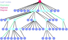
Explanation of the MST metrics: The MST is a subnetwork of the original network that does not contain loops or triangles. Here an MST is depicted, where the circles correspond to nodes and the (structural or functional) connections by lines. Leaf nodes, that is, end nodes with 1 connection (a degree of 1), are colored dark blue. The pink node is the node with the highest number of connections. The diameter is the longest shortest path in the network, here depicted in the connecting green lines. Two other measures that were computed are degree divergence (broadness of the degree distribution) and tree hierarchy. A low tree hierarchy corresponds to a more path‐like topology, whereas a high tree hierarchy to a more star‐like topology (see also Table 2). [Color figure can be viewed in the online issue, which is available at http://wileyonlinelibrary.com.]

Statistical Analysis

Statistical analyses of the cortical thickness correlation networks and its properties were performed in Matlab v2012a. Statistical analyses of functional connectivity and MST network properties were performed in SPSS 20.0 (Chicago, IL). Normality of the variables was assessed using the one‐sided Kolmogorov–Smirnov test and histogram inspection. P values < 0.05 were considered statistically significant. The analyses were performed in the following three stages: First, structural covariance networks were compared between groups; second, functional networks were compared; finally, the relationship between structural and functional networks was examined:

1. Structural covariance networks: raw correlation values together with all conventional and MST measures were compared using permutation analyses (1,000 permutations) [Bernhardt et al., 2011; Bullmore et al., 1999; He et al., 2008]. First, all conventional and MST measures were computed for structural networks of the MS and healthy control group. For each measure separately, the difference in values between healthy controls and MS patients was used as test‐statistic, and significance of the test‐static was determined by permutation testing: for each permutation (out of 1,000), group membership was randomly permuted for all subjects and cortical thickness correlations were recalculated for the permuted groups (see Estimation of Structural Covariance section). Next the test‐statistic was determined for each permutation, resulting in a distribution of permuted test‐statistic values. The measured test‐static was evaluated against this distribution, for which the 95 percentile points were considered to be critical. No covariance adjustment was necessary for further group comparisons as these effects were already removed before computation of cortical thickness correlations (see Estimation of Structural Covariance section).

2. Functional connectivity and functional networks: Average functional connectivity (i.e., mean PLI across nodes in the networks [before normalization]) was compared between the groups for each frequency band separately with regression analyses, including age and gender as covariates. When mean PLI differed between groups, regional PLI values were compared between groups as a post hoc analysis by means of permutation analysis [Nichols and Holmes, 2002].

   Here a null distribution for between‐group differences (independent t‐test) is derived by permuting group assignment and calculating a t‐statistic after each permutation. To correct for multiple comparisons, the maximum t‐value across ROIs for each permutation was used to construct a distribution of maximum t‐values for 1,000 permutations of group membership. The threshold at the 0.05 significance level (i.e., the 95th percentile point) for the distribution permuted values was determined. Average functional network properties (both conventional and MST) were compared between groups in each frequency band with regression analyses, including age and gender as covariates. For all analyses within a frequency band, we corrected for multiple comparisons with the false discovery rate procedure (six tests per frequency band) for the global tests [Benjamini and Hochberg, 1995].

3. Structural covariance versus functional networks: Third, we used the nonparametric Mantel test to quantify the relationship between structural covariance networks and MEG functional networks. To this end, we constructed a group‐level functional network by averaging the functional networks across epochs and subjects to obtain one 78 × 78 matrix per group for each frequency band. The correlation coefficient was computed between structural and functional connectivity measures across the AAL regions per group and frequency band. In addition, regional relationship between structural covariance and functional networks was measured by calculating the difference between the rank‐transformed structural covariance (SC _R) and the rank‐transformed group‐averaged functional networks (FC _R). We computed regional similarity between structural and functional connections by:

   $$\text{similarity}=〈1-\text{abs}\left[\mathbf{S}{\mathbf{C}}_{\mathrm{R}}-\mathbf{F}{\mathbf{C}}_{\mathrm{R}}\right]〉.$$ (5)

   here abs corresponds to the absolute value, and <> corresponds to the mean over all rows of the matrix to obtain a similarity index for each ROI. To test whether a similarity value for a ROI was significant, we used permutation analysis (1,000 permutations) where in each permutation the elements in the ranked structural covariance and averaged functional network matrices were randomized [Nichols and Holmes, 2002].

4. Regional cortical thickness versus functional networks: Last, we also analyzed the relationship between regional cortical thickness and functional networks. For each subject, we obtained cortical thickness values for each region. Then, we averaged each functional connectivity matrix over its rows and averaged across five epochs for each subject to obtain one functional connectivity (PLI) value for each region per subject. We then computed Pearson correlations for each region between cortical thickness and functional connectivity and corrected for the number of tests with the false discovery rate [Benjamini and Hochberg, 1995].

RESULTS

Table 2 reports the subject characteristics. MS and healthy controls differed in age, but not in their gender distribution. Patient group (67%) consisted of relapsing–remitting MS patients, 21% of secondary‐ and 12% primary‐progressive MS patients. MS patients showed significant reduction in mean cortical thickness and normalized gray matter volume (Table 1).

Table 2.

Demographic, clinical, and MRI measures for MS patients and healthy controls

	MS patients n = 102		Healthy controls n = 42		P value
	Mean	±SD	Mean	±SD
Age (in years)	54.23	9.76	51.14	5.98	0.023
Gender (F in %)	63.7%		61.9%		—
Disease type (RR/SP/PP)	68/22/12		—		—
Disease duration (years)	18.11	6.69	—		—
NBV (L)	1.41	0.09	1.49	0.07	<0.001
NGMV (L)	0.75	0.05	0.79	0.05	<0.001
NWMV (L)	0.66	0.04	0.69	0.03	<0.001
CT (mm)	2.48	0.10	2.56	0.08	<0.001
LV (mL)a	8.88	(3.37–17.92)		—	—
NLV (mL)a	10.51	(4.20–23.77)		—	—

RR, relapsing–remitting; SP, secondary‐progressive; PP, primary‐progressive; NBV, normalized brain volume; NGMV, normalized GM volume; NWMV, normalized white matter volume; CT, cortical thickness; LV, lesion volume; NLV, normalized lesion volume.

^avalues were not normally distributed; displayed median and (interquartile range).

Structural Covariance Networks

We first compared raw cortical thickness correlation values between the two groups and these were similar for MS patients and healthy subjects (permutation test: P = 0.8; MS patients median R = −0.0075, range R [0.75 to −0.42], healthy controls median R = −0.0074, range R [0.62 to −0.53]). In Figure 3, we depict the mean raw cortical thickness correlation per area, where it can be observed that these mean values are strongly affected by the large number of matrix elements with low correlations. Next, we compared network properties of the structural covariance networks between groups. The MS group displayed a higher normalized clustering (MS patients C _w = 1.05, healthy controls C _w = 1.04, P < 0.001) and a higher normalized shortest path length (MS patients L _w = 0.99 healthy controls L _w = 0.98, P < 0.001) compared to healthy controls, which is indicative of a more regular structural covariance network (Supporting Information Fig. S1). Finally, we compared the structural MST between groups, but we did not find differences in MST metrics between the groups (MS patients L _n = 0.36, d = 0.14, T _H = 0.32, K = 2.47, healthy controls L _n = 0.36, d = 0.14, T _H = 0.31, K = 2.39, all P > 0.05).

Figure 3.

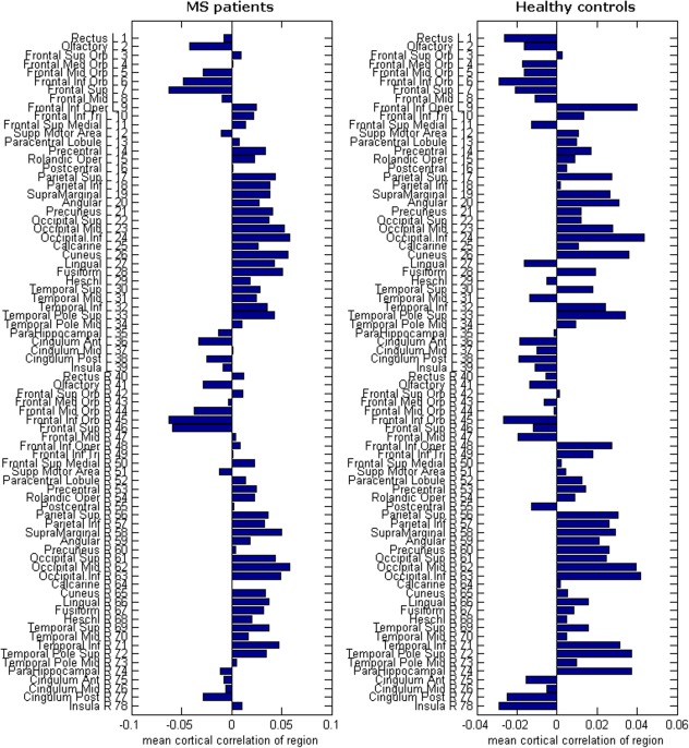
Mean cortical correlation values: Here we show the mean raw correlation value for each region. These values are obtained by averaging over all row elements of the structural covariance matrices in Supporting Information Figure S1. Depicted on the right of the horizontal bar plots are the corresponding AAL regions. The number next to each name also corresponds to the numbers in Supporting Information Figure S1. [Color figure can be viewed in the online issue, which is available at http://wileyonlinelibrary.com.]

Functional Connectivity and Functional Networks

To investigate differences in functional connectivity between the two groups, we compared the mean PLI values for each frequency band between MS patients and healthy controls. First of all, MS patients showed higher mean PLI values in the delta and theta band, and lower mean PLI values in the alpha2 band than healthy controls (Table 3). Figure 4 shows that in the delta band, higher PLI values were present in many cortical areas, except for right‐temporal and occipital areas. In the theta band, MS patients showed higher PLI values in many cortical areas including occipital, temporal, parietal, and frontal areas. In the alpha2 band, PLI values for MS patients were lower in, among other regions, the occipital, temporal, and parietal areas.

Table 3.

Comparative analyses of mean functional connectivity between MS patients and healthy controls

	MS patients	Healthy controls	Standardized B	t value	P value
Mean PLI
Delta	0.113 ± 0.004	0.106 ± 0.004	−0.56	−7.90	<0.001
Theta	0.098 ± 0.004	0.094 ± 0.004	−0.56	−7.89	<0.001
Alpha1	0.138 ± 0.007	0.138 ± 0.006	−0.10	−0.12	0.9
Alpha2	0.112 ± 0.006	0.115 ± 0.006	0.22	2.72	0.007
Beta	0.064 ± 0.005	0.065 ± 0.004	0.04	0.47	0.6
Gamma	0.048 ± 0.002	0.049 ± 0.002	0.04	0.47	0.6

Bold = significant after correcting for multiple comparisons by the FDR. PLI, phase lag index; MST, minimum spanning tree.

Values listed are mean ± SD.

Figure 4.

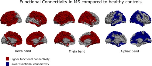
Functional connectivity: Regional functional connectivity differences between MS patients and healthy controls in the delta, theta, and alpha2 band. Here, a brain map is depicted where for each ROI the regional functional connectivity is shown, defined as the average functional connectivity between that ROI and all other ROIs. Higher functional connectivity (red color) in the MS patients is present in both the delta and theta band. Compared to the delta band, frontal cortical areas are spared in the theta band, whereas occipital, temporal, and parietal areas are more affected. Lower functional connectivity (blue color) is present in the alpha2 band, especially in temporal, occipital and parietal regions. [Color figure can be viewed in the online issue, which is available at http://wileyonlinelibrary.com.]

Conventional network analysis revealed a higher normalized path length in the theta band and a lower normalized clustering in the alpha2 band in MS patients (Table 4). This indicates that network topology tends to become more regular in the theta band, in contrast to more random topology in the alpha2 band. MST analyses revealed that MST topology was only different in the alpha2 band for MS patients. This was reflected in a significantly lower leaf fraction, lower degree divergence, and lower tree hierarchy in this frequency band for MS patients (Table 4 and Fig. 5).

Table 4.

Comparative analyses of functional network properties between MS patients and healthy controls

		MS patients	Healthy controls	Standardized B	t value	P value
Delta	Normalized clustering coefficient	1.0076 ± 0.0017	1.0076 ± 0.0013	−0.009	−1.03	0.91
	Normalized path length	1.016 ± 0.017	1.012 ± 0.016	−0.154	−1.83	0.069
	MST leaf fraction	0.53 ± 0.022	0.53 ± 0.021	0.011	0.13	0.89
	MST tree hierarchy	0.403 ± 0.023	0.403 ± 0.021	−0.010	−0.12	0.91
	MST degree divergence	3.1 ± 0.17	3.16 ± 0.17	0.12	1.41	0.16
	MST diameter	17 ± 1.2	17 ± 1.1	−0.032	−0.38	0.71
Theta	Normalized clustering coefficient	1.0073 ± 0.0016	1.0068 ± 0.0016	−0.13	−1.55	0.12
	Normalized path length	1.016 ± 0.013	1.0084 ± 0.012	−0.27	−3.22	0.002
	MST leaf fraction	0.53 ± 0.024	0.53 ± 0.024	−0.009	−0.11	0.91
	MST tree hierarchy	0.403 ± 0.023	0.405 ± 0.017	0.043	0.51	0.61
	MST degree divergence	3.1 ± 0.15	3.1 ± 0.19	−0.059	−0.71	0.48
	MST diameter	17 ± 1.4	17 ± 1.4	0.15	1.76	0.081
Alpha2	Normalized clustering coefficient	1.0077 ± 0.0019	1.0084 ± 0.0018	0.19	2.24	0.027
	Normalized path length	1.014 ± 0.014	1.013 ± 0.014	−0.061	−0.72	0.40
	MST leaf fraction	0.53 ± 0.021	0.54 ± 0.020	0.23	2.74	0.007
	MST tree hierarchy	0.40 ± 0.019	0.41 ± 0.021	0.22	2.64	0.009
	MST degree divergence	3.1 ± 0.18	3.2 ± 0.14	0.17	2.09	0.039
	MST diameter	17 ± 1.2	17 ± 1.1	−0.11	−1.29	0.20

Bold = significant after correcting for multiple comparisons by the FDR. MST, minimum spanning tree.

Values listed are mean ± SD.

Figure 5.

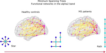
MST results for functional networks in the alpha2 band: For illustrative purposes, the average MSTs across subjects for MS patients and healthy controls are depicted. The diameter of the circles in the glass brains is proportional to the degree of the nodes in the MST; the color of the lines connecting the circles indicates the strength of the functional connections, with warmer colors indicating stronger connections. The MST for MS patients was characterized by a shift toward a more path‐like topology reflected by a lower leaf fraction, lower degree divergence, and lower tree hierarchy. [Color figure can be viewed in the online issue, which is available at http://wileyonlinelibrary.com.]

Table 5.

Correlations between cortical thickness correlations and functional connectivity

Frequency bands	MS patients	Healthy controls
Delta band	R = −0.01	R = 0.09
	P = 0.7	P = 0.001
Theta band	R = 0.17	R = −0.004
	P = 0.001	P = 0.6
Alpha2 band	R = 0.13	R = 0.10
	P = 0.001	P = 0.001

Bold = significant after correcting for multiple comparisons by the FDR.

R, Mantel's correlation coefficient, P, P‐value.

Structural Covariance Versus Functional Networks

In the previous analyses, we have demonstrated that both the structural covariance and functional networks get disrupted in MS. Note that the direction of the shift in topology was the same for the structural covariance network and the functional networks in the theta band. Both these networks were characterized by more regular organization, which was indicated by higher normalized path length and higher normalized clustering. However, functional networks in the alpha2 band showed a change in the opposite direction as these networks were characterized by a more random network organization.

To further characterize the relationship between structural covariance and functional network alterations in MS, we further performed stratified correlation analyses for the MEG frequency bands where we found significant differences in functional connectivity between MS patients and controls. We found that correlations between structural covariance and functional networks depend on frequency band and group as there were weak but significant positive correlations between the two in the delta and alpha2 band for healthy controls and in the theta and alpha2 band for MS patients. Additional analyses revealed that these associations between the two types of networks were both driven by negative as well as positive cortical thickness correlations (Supporting Information Table S2).

To zoom into regional relationship between structural and functional networks, we computed the regional similarity between the two (Fig. 6). In the delta band, we observed more regions in the healthy subject group that showed high similarity between structural covariance and functional connectivity than in the MS patient group. In the theta band, we observed the opposite; regional similarity was more prominent in MS patients, in particular for posterior and temporal regions. This pattern was also observed in the alpha2 band for both groups, only less prominent than in the theta band.

Figure 6.

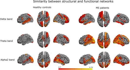
Regional similarity: To quantify the regional overlap between structural and functional networks, we computed a similarity measure as defined in Eq. (6) (see Methods). Color coded maps of the similarity for each region are shown for different frequency bands. Colors were attributed to a region only if the similarity between modalities for that region was significant. Red indicates relatively low similarity and yellow indicates relatively high similarity. We observed that the similarity was especially high in temporo‐posterior regions in MS patients (in the theta and alpha2 band), as well as for healthy subjects in the alpha2. [Color figure can be viewed in the online issue, which is available at http://wileyonlinelibrary.com.]

Regional Cortical Thickness Versus Functional Networks

Finally, we analyzed the relationship between regional cortical thickness and functional networks by computing pair‐wise correlations to investigate if the relationship between structural covariance and functional networks can be explained by merely regional thickness values alone. We found correlations of weak strength in, for example, the alpha2 band, however, none of these correlations survived correction for multiple hypothesis testing (Supporting Information Table S1).

DISCUSSION

The current study aimed to investigate how structural covariance and MEG functional networks were affected by the disease within the same MS sample. Our main findings were: (1) MS patients and healthy controls showed similar average structural covariance; (2) MS patients showed higher functional connectivity in the delta and theta band and lower functional connectivity in the alpha2 band; (3) structural covariance networks and functional networks in the theta band in MS patients were more regularly organized than in controls; (4) functional networks in the alpha2 band were more randomly organized in MS than in controls; and (5) the relationship between structural covariance and MEG functional networks was dependent on the frequency band and on group membership, particularly in the theta band.

Structural Covariance Networks

Structural network analyses revealed a spatial reconfiguration of interregional cortical thickness associations in MS that did not effect the average correlation across all areas. This reconfiguration resulted in a more regular topology in the MS group, as indicated by higher normalized clustering and path length values. At this point, it is still unclear as to what mechanisms underlie the existence of cortical thickness correlations. One hypothesis is that they might arise as a consequence of tension exerted by axonal connectivity between two brain areas [van Essen, 1997]. Another structural covariance study has previously reported similar findings of lower global efficiency (the inverse of path length) in MS patients, and they showed that this finding was proportional to white matter lesion load [He et al., 2009]. This finding suggests that damage to white matter tracts that connect cortical areas influence the cortical thickness correlations, supporting the axonal tension hypothesis [Gong et al., 2012; Li et al., 2012; Shu et al., 2011]. However, one other study demonstrated that white matter tracts explain only a part of cortical thickness correlations (30%–40%) [Gong et al., 2012], suggesting that other factors are implicated in cortical thickness correlations. It has been suggested that cortical thickness correlations reflect synchronized maturation between brain areas and are not only influenced by white matter connections but also by functional coactivation [Alexander‐Bloch et al., 2013a, b].

Functional Connectivity and Functional Networks

Here we report that in comparison to healthy controls MS patients showed higher functional connectivity in the delta and theta band and lower functional connectivity in the alpha2 band. Our finding of higher functional connectivity in the theta band and lower functional connectivity in the alpha2 band in the MS group is in line with previous reports [Cover et al., 2006; Leocani et al., 2000; Schoonheim et al., 2011; Tewarie et al., 2013aa]. Higher functional connectivity in the delta band in MS patients has not been reported before. Possibly this increase in MS is related to the disease duration of patients in our sample, which was longer than patients sampled in previous MEG studies [Cover et al., 2006; Schoonheim et al., 2011; Tewarie et al., 2013a]. It is well‐known from other neurological diseases such as Parkinson's and Alzheimer's disease, which changes in the delta band are more prominent in later stages of the disease [Bosboom et al., 2009a, b; de Haan et al., 2008]. At this point, it is still unclear what the relationship of higher functional connectivity in this band with cognitive functioning in MS is, but delta band oscillations in healthy subjects have been linked to decision making [Nacher et al., 2013],

Conventional functional network analyses revealed a higher path length in the theta band and lower clustering in the alpha2 band in MS patients compared to healthy controls. This indicates that functional networks in the theta band were less integrated (i.e., more regular), and in the alpha2 band less segregated (i.e., more random). MST differences between MS and control subjects were especially found in the alpha2 band, reflected by a lower MST leaf fraction, MST degree divergence and MST tree hierarchy in MS patients. An important aspect in complex networks is efficient communication between all nodes. This requires a small network diameter and simultaneous prevention of overloading of the central nodes. MST tree hierarchy measures the extent to which a tree displays this optimal configuration. In the present study, we found that functional networks in MS in the alpha2 band tend to shift away from this optimum level of hierarchy, toward a more path‐like topology and thus a less integrated network. These results replicate our previous finding in an earlier MEG study of lower MST leaf fraction, MST degree divergence, and MST tree hierarchy, which was related to worse cognitive performance in MS patients [Tewarie et al., 2013b]. Here we studied a different sample that only included relapsing–remitting MS patients and patients with shorter disease duration.

Previous MEG studies using MSTs in other neurological diseases such as Parkinson's disease and neuroglioma have demonstrated that shifts toward a more path‐like tree topology are signs of maladaptation and that these shifts are related to worse clinical outcome [Diessen et al., 2013; Olde Dubbelink et al., 2014; van Dellen et al., 2014]. Our present findings seem to be in line with these results, which may suggest that neurological diseases have a final common pathway in terms of the MST. These MST findings may help to overcome contradictory findings that have been obtained with conventional network analyses in neurological diseases, as has been reported for Alzheimer's disease and epilepsy [Diessen et al., 2013; Tijms et al., 2013]. These contradictory findings could be caused by the fact that conventional measures mix information about network topology and connectivity. The MST, in contrast, is insensitive to these confounds. In EEG studies, it has also been shown that the MST is sensitive to changes in network topology, rather than functional connectivity, in various cohorts and conditions, ranging from epilepsy, propofol‐induced anesthesia, schizophrenia, network maturation during childhood, or changes in motor function [Boersma et al., 2012; Demuru et al., 2013; Lee et al., 2006, 2010; Ortega et al., 2008; Schoen et al., 2011]. For a thorough review about the use of MSTs in brain network analysis, we refer to [Stam et al., 2014].

Structural Covariance Versus Functional Networks

We observed that brain regions that covary in thickness were also related by functional interactions in MS. Importantly, this relationship could not be found by pairwise correlations between regional gray matter thickness and regional functional connectivity. This indicates that changes in functional connectivity to a region in MS cannot be explained by a simple process of gray matter atrophy of that same region, but only if atrophy of this region is associated with atrophy elsewhere. One of the hypothesis to explain the presence of structural covariance is that these occur due to common and coordinated synaptogenesis in brain regions [Alexander‐Bloch et al., 2013a]. This coordinated synaptogenesis is probably influenced by genetics and by developmental relationships between cell‐types and cortical layers. However, also synchronous firing between regions and neuronal populations can induce synaptogenesis [Katz and Shatz, 1996]. This process may underlie the finding that we found associations between functional interactions and covariation in cortical thickness in healthy controls as well as MS patients.

The relationship between covariation in thickness and functional connectivity depended on group membership and frequency band. There seemed to be a shift in MS patients as within this group there was no association between the two in the delta band but appeared in the theta band. The shift of the association between functional connectivity and covariation in thickness across frequency bands may be related to changes in the anatomy of cortical layers: from neurophysiology studies, we know that infragranular cortical layers are more involved in generation of delta oscillations and supragranular cortical layers more in the generation of theta oscillations [Roopun et al., 2008]. Although speculation, this might indicate that covariation in thickness in MS is a process that is more associated with covariation of supragranular cortical layers and as a result of which the relationship between structural covariance and theta band functional connectivity increases. If we assume that infragranular layers are associated with delta band oscillations than factors such as retrograde axonal degeneration of infragranular layers due to white matter lesions may lead to decrease in delta band functional connectivity. Longitudinal and animal studies are required to test these hypotheses in the future.

When examining graph theoretical findings of the structural covariance and functional networks side by side, we observed that topological changes for structural covariance and functional networks in MS point in the same direction for the theta band, that is, they become more regular. In contrast, we observed that functional networks in MS in the alpha2 band tend to become more random, which is in the opposite direction of the (more regular) structural covariance network. Although this seems to be contradictory, a modeling study has revealed that the relationship between structural and functional network topology is in general nontrivial and may depend on local and global characteristics of neuronal populations.

To understand the relationship between structural covariance and functional networks, there is a need for a theoretical framework. For anatomical networks (based on physical connections rather than covariance of cortical thickness) and functional networks, such a framework has been investigated using various computational and analytical models [Deco et al., 2013; Honey et al., 2009; Tewarie et al., 2014; Zemanova et al., 2006]. We recently reported that functional connectivity can be understood by taking into account the degree product between anatomically connected nodes and the Euclidean distance between brain regions [Tewarie et al., 2014]. Also for structural covariance networks, there seem to be strong correlations for ROIs with short distance connections (along the diagonal of the structural connectivity matrices, see Supporting Information Fig. S1). Using the distance versus degree model (Supporting Information) it can be observed that both the distance between regions and the degree product in the structural covariance networks are able to explain functional connectivity in MS patients and healthy controls (Supporting Information Tables S3 and S4). Together, these results suggest that nearby ROIs with similar cortical thickness variations may also be functionally related, if there is an anatomical connection present. It should be noted though that the causal direction of these relationships is as yet unclear; future empirical and theoretical studies need to investigate the relationship between structural covariance‐, structural connection‐, and functional networks further.

Methodological Considerations

Some limitations apply to this work. First, in the MEG source space analysis, we selected the time‐series of one voxel as a representation for the whole ROI. This is a reduction of data, which may lead to loss of information. However, averaging over voxels in a ROI could introduce biases due to differences in ROI size leading to time‐series having different signal‐to‐noise‐ratios. Given these and other biases with averaging over sources, we chose to adhere to methods used previously in our group [Hillebrand et al., 2012; Tewarie et al., 2013b]. Second, in the present study, we obtained structural networks at the group‐level while we obtained functional networks at the subject‐level. This limits the analysis of the within subject relation between structure and function. To be able to interpret results within the context of previous studies, we performed group‐level structural covariance networks. For future research, we will compute single‐subject structural networks [Tijms et al., 2012]. Third, in the present study, we did not analyze medication effects or potential network differences due to the disease type (relapsing–remitting onset vs. progressive onset), since there was heterogeneous use of medication and the number of progressive onset MS patients was too low to reliably estimate structural covariance networks. We further need to mention that we did not predict clinical or cognitive dysfunction using the present data as this was not the aim of this article. Fourth, in the present study, we have focused on global aspects of the structural and functional networks. Future studies will also need to focus more on local properties of brain networks in MS, such as long distance correlations between individual nodes. Last, network analyses are accompanied with methodological difficulties such as differences in measurement scale across imaging modalities. To counter these difficulties, we removed scale effects by normalizing the weighted networks by its mean value, but this does not solve the influence of differences in the range of correlation values between two networks. The MST approach seems to be a valuable approach for the comparison of multimodal networks, as it does not suffer from these normalization problems.

CONCLUSION

Both gray matter atrophy and disruption of functional brain networks are hypothesized to be important pathological substrates for physical disability and cognitive dysfunction in MS. The relationship between these pathological alterations is poorly understood, but clarifying this relationship could give more insight into disease mechanisms in MS. In the present study, we aimed to bridge the gap between these two important pathological substrates of the disease. In the present cohort, we clearly demonstrated that alterations of functional connectivity in MS cannot be simply explained by regional gray matter atrophy itself as we have shown that localized measurements fail to take into account the inherent connectivity structure of the brain. Changes in functional network connectivity in MS could only be partially explained if complex and coordinated patterns of gray matter atrophy were taken into account. We have subsequently showed that there can be a complex interplay between these structural covariance networks and functional networks in MS. Our work is a first step toward a better understanding of how differential pathological alterations are related to each other in MS.

Supporting information

Supplementary Information

Supplementary Information

Supplementary Information

Supplementary Information

REFERENCES

- Alexander‐Bloch A, Giedd JN, Bullmore E (2013a): Imaging structural co‐variance between human brain regions. Nat Rev Neurosci 14:322–336. [DOI] [PMC free article] [PubMed] [Google Scholar]
- Alexander‐Bloch A, Raznahan A, Bullmore E, Giedd J (2013b): The convergence of maturational change and structural covariance in human cortical networks. J Neurosci 33:2889–2899. [DOI] [PMC free article] [PubMed] [Google Scholar]
- Ashburner J, Friston KJ (2005): Unified segmentation. Neuroimage 26:839–851. [DOI] [PubMed] [Google Scholar]
- Barrat A, Barthelemy M, Vespignani A (2008): Networks and complexity. Dynamical processes on complex networks, Cambridge University Press, New York, pp 24–49. [Google Scholar]
- Benjamini Y, Hochberg Y (1995): Controlling the false discovery rate: A practical and powerful approach to multiple testing. J R Stat Soc 57:289–300. [Google Scholar]
- Bernhardt BC, Chen Z, He Y, Evans AC, Bernasconi N (2011): Graph‐theoretical analysis reveals disrupted small‐world organization of cortical thickness correlation networks in temporal lobe epilepsy. Cereb Cortex 21:2147–2157. [DOI] [PubMed] [Google Scholar]
- Boersma M, Smit DJ, Boomsma DI, Geus EJ, Delemarre‐van de Waal HA, Stam C (2012): Growing trees in child brains: Graph theoretical analysis of EEG derived minimum spanning tree in 5 and 7 year old children reflects brain maturation. Brain Connect 3:50–60. [DOI] [PubMed] [Google Scholar]
- Bosboom JL, Stoffers D, Stam CJ, Berendse HW, Wolters EC (2009a): Cholinergic modulation of MEG resting‐state oscillatory activity in Parkinson's disease related dementia. Clin Neurophysiol 120:910–915. [DOI] [PubMed] [Google Scholar]
- Bosboom JL, Stoffers D, Wolters EC, Stam CJ, Berendse HW (2009b): MEG resting state functional connectivity in Parkinson's disease related dementia. J Neural Transm 116:193–202. [DOI] [PubMed] [Google Scholar]
- Bullmore E, Sporns O (2009): Complex brain networks: Graph theoretical analysis of structural and functional systems. Nat Rev Neurosci 10:186–198. [DOI] [PubMed] [Google Scholar]
- Bullmore ET, Suckling J, Overmeyer S, Rabe‐Hesketh S, Taylor E, Brammer MJ (1999): Global, voxel, and cluster tests, by theory and permutation, for a difference between two groups of structural MR images of the brain. IEEE Trans Med Imaging 18:32–42. [DOI] [PubMed] [Google Scholar]
- Calabrese M, Atzori M, Bernardi V, Morra A, Romualdi C, Rinaldi L, McAuliffe MJ, Barachino L, Perini P, Fischl B, Battistin L, Gallo P (2007): Cortical atrophy is relevant in multiple sclerosis at clinical onset. J Neurol 254:1212–1220. [DOI] [PubMed] [Google Scholar]
- Calabrese M, Filippi M, Gallo P (2010): Cortical lesions in multiple sclerosis. Nat Rev Neurol 6:438–444. [DOI] [PubMed] [Google Scholar]
- Cover KS, Vrenken H, Geurts JJ, van Oosten BW, Jelles B, Polman CH, Stam CJ, vanDijk BW (2006): Multiple sclerosis patients show a highly significant decrease in alpha band interhemispheric synchronization measured using MEG. Neuroimage 29:783–788. [DOI] [PubMed] [Google Scholar]
- Dale AM, Fischl B, Sereno MI (1999): Cortical surface‐based analysis. I. Segmentation and surface reconstruction. Neuroimage 9:179–194. [DOI] [PubMed] [Google Scholar]
- de Haan W, Stam CJ, Jones BF, Zuiderwijk IM, van Dijk BW, Scheltens P (2008): Resting‐state oscillatory brain dynamics in Alzheimer disease. J Clin Neurophysiol 25:187–193. [DOI] [PubMed] [Google Scholar]
- de Haan W, van der Flier WM, Wang H, Van Mieghem PF, Scheltens P, Stam C (2012): Disruption of functional brain networks in Alzheimer's disease: What can we learn from graph spectral analysis of resting‐state MEG? Brain Connect 2:45–55. [DOI] [PubMed] [Google Scholar]
- Deco G, Ponce‐Alvarez A, Mantini D, Romani GL, Hagmann P, Corbetta M (2013): Resting‐state functional connectivity emerges from structurally and dynamically shaped slow linear fluctuations. J Neurosci 33:11239–11252. [DOI] [PMC free article] [PubMed] [Google Scholar]
- Demuru M, Fara F, Fraschini M (2013): Brain network analysis of EEG functional connectivity during imagery hand movements. J Integr Neurosci 12:441–447. [DOI] [PubMed] [Google Scholar]
- Desikan RS, Segonne F, Fischl B, Quinn BT, Dickerson BC, Blacker D, Buckner RL, Dale AM, Maguire RP, Hyman BT, Albert MS, Killiany RJ (2006): An automated labeling system for subdividing the human cerebral cortex on MRI scans into gyral based regions of interest. Neuroimage 31:968–980. [DOI] [PubMed] [Google Scholar]
- Diessen E, Diederen SJ, Braun KP, Jansen FE, Stam CJ (2013): Functional and structural brain networks in epilepsy: What have we learned? Epilepsia 54:1855–1865. [DOI] [PubMed] [Google Scholar]
- Douw L, de GM , DE, van Aronica E, Heimans JJ, Klein M, Stam CJ, Reijneveld JC, Hillebrand A (2013): Local MEG networks: The missing link between protein expression and epilepsy in glioma patients? Neuroimage 75:195–203. [DOI] [PubMed] [Google Scholar]
- Fischl B, Sereno MI, Dale AM (1999): Cortical surface‐based analysis. II: Inflation, flattening, and a surface‐based coordinate system. Neuroimage 9:195–207. [DOI] [PubMed] [Google Scholar]
- Fornito A, Zalesky A, Breakspear M (2013): Graph analysis of the human connectome: Promise, progress, and pitfalls. Neuroimage 80C:426–444. [DOI] [PubMed] [Google Scholar]
- Friston KJ, Holmes P, Worsley KJ, Poline JP, Frith CD, Frackowiak RSJ (2004): Statistical parametric maps in functional imaging: A general linear approach. Human Brain Mapping 2:189–210. [Google Scholar]
- Gamboa OL, Tagliazucchi E, WF, von Jurcoane A, Wahl M, Laufs H, Ziemann U (2014): Working memory performance of early MS patients correlates inversely with modularity increases in resting state functional connectivity networks. Neuroimage 94:385–395. [DOI] [PubMed] [Google Scholar]
- Geurts JJ, Barkhof F (2008): Grey matter pathology in multiple sclerosis. Lancet Neurol 7:841–851. [DOI] [PubMed] [Google Scholar]
- Gong G, He Y, Concha L, Lebel C, Gross DW, Evans AC, Beaulieu C (2009): Mapping anatomical connectivity patterns of human cerebral cortex using in vivo diffusion tensor imaging tractography. Cereb Cortex 19:524–536. [DOI] [PMC free article] [PubMed] [Google Scholar]
- Gong G, He Y, Chen ZJ, Evans AC (2012): Convergence and divergence of thickness correlations with diffusion connections across the human cerebral cortex. Neuroimage 59:1239–1248. [DOI] [PubMed] [Google Scholar]
- Hardmeier M, Schoonheim MM, Geurts JJ, Hillebrand A, Polman CH, Barkhof F, Stam CJ (2012): Cognitive dysfunction in early multiple sclerosis: Altered centrality derived from resting‐state functional connectivity using magneto‐encephalography. PLoS One 7:e42087. [DOI] [PMC free article] [PubMed] [Google Scholar]
- He Y, Chen ZJ, Evans AC (2007): Small‐world anatomical networks in the human brain revealed by cortical thickness from MRI. Cereb Cortex 17:2407–2419. [DOI] [PubMed] [Google Scholar]
- He Y, Chen Z, Evans A (2008): Structural insights into aberrant topological patterns of large‐scale cortical networks in Alzheimer's disease. J Neurosci 28:4756–4766. [DOI] [PMC free article] [PubMed] [Google Scholar]
- He Y, Dagher A, Chen Z, Charil A, Zijdenbos A, Worsley K, Evans A (2009): Impaired small‐world efficiency in structural cortical networks in multiple sclerosis associated with white matter lesion load. Brain 132:3366–3379. [DOI] [PMC free article] [PubMed] [Google Scholar]
- Hillebrand A, Barnes GR (2005): Beamformer analysis of MEG data. Int Rev Neurobiol 68:149–171. [DOI] [PubMed] [Google Scholar]
- Hillebrand A, Barnes GR, Bosboom JL, Berendse HW, Stam CJ (2012): Frequency‐dependent functional connectivity within resting‐state networks: An atlas‐based MEG beamformer solution. Neuroimage 59:3909–3921. [DOI] [PMC free article] [PubMed] [Google Scholar]
- Honey CJ, Sporns O, Cammoun L, Gigandet X, Thiran JP, Meuli R, Hagmann P (2009): Predicting human resting‐state functional connectivity from structural connectivity. Proc Natl Acad Sci USA 106:2035–2040. [DOI] [PMC free article] [PubMed] [Google Scholar]
- Katz LC, Shatz CJ (1996): Synaptic activity and the construction of cortical circuits. Science 274:1133–1138. [DOI] [PubMed] [Google Scholar]
- Kruskal J (1956): On the shortest spanning subtree of a graph and the traveling salesman problem. Proc Am Math Soc 7:48–50. [Google Scholar]
- Leocani L, Locatelli T, Martinelli V, Rovaris M, Falautano M, Filippi M, Magnani G, Comi G (2000): Electroencephalographic coherence analysis in multiple sclerosis: correlation with clinical, neuropsychological, and MRI findings. J Neurol Neurosurg Psychiatry 69:192–198. [DOI] [PMC free article] [PubMed] [Google Scholar]
- Lee U, Kim S, Jung KY (2006): Classification of epilepsy types through global network analysis of scalp electroencephalograms. Phys Rev E Stat Nonlin Soft Matter Phys 73:041920. [DOI] [PubMed] [Google Scholar]
- Lee U, Oh G, Kim S, Noh G, Choi B, Mashour GA (2010): Brain networks maintain a scale‐free organization across consciousness, anesthesia, and recovery: Evidence for adaptive reconfiguration. Anesthesiology 113:1081. [DOI] [PMC free article] [PubMed] [Google Scholar]
- Li Y, Jewells V, Kim M, Chen Y, Moon A, Armao D, Troiani L, Markovic‐Plese S, Lin W, Shen D (2012): Diffusion tensor imaging based network analysis detects alterations of neuroconnectivity in patients with clinically early relapsing‐remitting multiple sclerosis. Hum Brain Mapp 34:3376–3391. [DOI] [PMC free article] [PubMed] [Google Scholar]
- Louapre C, Perlbarg V, Garcia‐Lorenzo D, Urbanski M, Benali H, Assouad R, Galanaud D, Freeman L, Bodini B, Papeix C, Tourbah A, Lubetzki C, Lehericy S, Stankoff B (2014): Brain networks disconnection in early multiple sclerosis cognitive deficits: An anatomofunctional study. Hum Brain Mapp [DOI] [PMC free article] [PubMed] [Google Scholar]
- Nacher V, Ledberg A, Deco G, Romo R (2013): Coherent delta‐band oscillations between cortical areas correlate with decision making. Proc Natl Acad Sci USA 110:15085–15090. [DOI] [PMC free article] [PubMed] [Google Scholar]
- Nichols TE, Holmes AP (2002): Nonparametric permutation tests for functional neuroimaging: A primer with examples. Hum Brain Mapp 15:1–25. [DOI] [PMC free article] [PubMed] [Google Scholar]
- Olde Dubbelink KT, Hillebrand A, Stoffers D, Deijen JB, Twisk JW, Stam CJ, Berendse HW (2014): Disrupted brain network topology in Parkinson's disease: A longitudinal magnetoencephalography study. Brain 137:197–207. [DOI] [PubMed] [Google Scholar]
- Ortega GJ, Sola RG, Pastor J (2008): Complex network analysis of human ECoG data. Neurosci Lett 447:129–133. [DOI] [PubMed] [Google Scholar]
- Robinson SE, Vrba J (1999):Functional neuroimaging by synthetic aperture magnetometry In:Yoshimoto M, Kotani S, Kuriki H, Karibe N, Nakatato E, editors. Recent Advances in Biomagnetism. Sendai: Tohoku University Press, pp 302–305. [Google Scholar]
- Roopun AK, Kramer MA, Carracedo LM, Kaiser M, Davies CH, Traub RD, Kopell NJ, Whittington MA (2008): Temporal interactions between cortical rhythms. Front Neurosci 2:145–154. [DOI] [PMC free article] [PubMed] [Google Scholar]
- Rubinov M, Sporns O (2010): Complex network measures of brain connectivity: Uses and interpretations. Neuroimage 52:1059–1069. [DOI] [PubMed] [Google Scholar]
- Schoen W, Chang JS, Lee U, Bob P, Mashour GA (2011): The temporal organization of functional brain connectivity is abnormal in schizophrenia but does not correlate with symptomatology. Conscious Cogn 20:1050–1054. [DOI] [PubMed] [Google Scholar]
- Schoonheim MM, Geurts JJ, Landi D, Douw L, van der Meer ML, Vrenken H, Polman CH, Barkhof F, Stam CJ (2011): Functional connectivity changes in multiple sclerosis patients: A graph analytical study of MEG resting state data. Hum Brain Mapp 34:52–61. [DOI] [PMC free article] [PubMed] [Google Scholar]
- Shu N, Liu Y, Li K, Duan Y, Wang J, Yu C, Dong H, Ye J, He Y (2011): Diffusion tensor tractography reveals disrupted topological efficiency in white matter structural networks in multiple sclerosis. Cereb Cortex 21:2565–2577. [DOI] [PubMed] [Google Scholar]
- Stam CJ, van Straaten EC (2012): The organization of physiological brain networks. Clin Neurophysiol 123:1067–1087. [DOI] [PubMed] [Google Scholar]
- Stam CJ, Nolte G, Daffertshofer A (2007): Phase lag index: Assessment of functional connectivity from multi channel EEG and MEG with diminished bias from common sources. Hum Brain Mapp 28:1178–1193. [DOI] [PMC free article] [PubMed] [Google Scholar]
- Stam CJ, Tewarie P, DE, van van Straaten EC, Hillebrand A, Van MP (2014): The trees and the forest: Characterization of complex brain networks with minimum spanning trees. Int J Psychophysiol 92:129–138. [DOI] [PubMed] [Google Scholar]
- Steenwijk MD, Daams M, Pouwels PJ, Balk LJ, Tewarie PK, Killestein J, Uitdehaag BM, Geurts JJ, Barkhof F, Vrenken H (2014): What explains gray matter atrophy in long‐standing multiple sclerosis? Radiology 132708. [DOI] [PubMed] [Google Scholar]
- Taulu S, Simola J (2006): Spatiotemporal signal space separation method for rejecting nearby interference in MEG measurements. Phys Med Biol 51:1759–1768. [DOI] [PubMed] [Google Scholar]
- Taulu S, Hari R (2009): Removal of magnetoencephalographic artifacts with temporal signal‐space separation: demonstration with single‐trial auditory‐evoked responses. Hum Brain Mapp 30:1524–1534. [DOI] [PMC free article] [PubMed] [Google Scholar]
- P Tewarie, MM Schoonheim, CJ Stam, ML van der Meer, BW van Dijk, F Barkhof, CH Polman, A Hillebrand (2013a): Cognitive and clinical dysfunction, altered MEG resting‐state networks and thalamic atrophy in multiple sclerosis. PLoS One 8:e69318. [DOI] [PMC free article] [PubMed] [Google Scholar]
- Tewarie P, Hillebrand A, Schoonheim MM, van Dijk BW, Geurts JJG, Barkhof F, Polman CH, Stam CJ (2013b): Functional brain network analysis using minimum spanning trees in Multiple Sclerosis: An MEG source‐space study. Neuroimage 88:308–318. [DOI] [PubMed] [Google Scholar]
- Tewarie P, Hillebrand A, DE, van Schoonheim MM, Barkhof F, Polman CH, Beaulieu C, Gong G, van Dijk BW, Stam CJ (2014): Structural degree predicts functional network connectivity: A multimodal resting‐state fMRI and MEG study. Neuroimage 97:296–307. [DOI] [PubMed] [Google Scholar]
- Tijms BM, Series P, Willshaw DJ, Lawrie SM (2012): Similarity‐based extraction of individual networks from gray matter MRI scans. Cereb Cortex 22:1530–1541. [DOI] [PubMed] [Google Scholar]
- Tijms BM, Wink AM, HW, de van der Flier WM, Stam CJ, Scheltens P, Barkhof F (2013): Alzheimer's disease: Connecting findings from graph theoretical studies of brain networks. Neurobiol Aging 34:2023–2036. [DOI] [PubMed] [Google Scholar]
- Tzourio‐Mazoyer N, Landeau B, Papathanassiou D, Crivello F, Etard O, Delcroix N, Mazoyer B, Joliot M (2002): Automated anatomical labeling of activations in SPM using a macroscopic anatomical parcellation of the MNI MRI single‐subject brain. Neuroimage 15:273–289. [DOI] [PubMed] [Google Scholar]
- van Essen DC (1997): A tension‐based theory of morphogenesis and compact wiring in the central nervous system. NATURE‐LONDON 313–318. [DOI] [PubMed] [Google Scholar]
- van Dellen E., Douw L, Hillebrand A, de Witt Hamer PC, Baayen JC, Heimans JJ, Reijneveld JC, Stam CJ (2014): Epilepsy surgery outcome and functional network alterations in longitudinal MEG: A minimum spanning tree analysis. Neuroimage 86:354–363. [DOI] [PubMed] [Google Scholar]
- van Wijk BC, Stam CJ, Daffertshofer A (2010): Comparing brain networks of different size and connectivity density using graph theory. PLoS One 5:e13701. [DOI] [PMC free article] [PubMed] [Google Scholar]
- Watts DJ, Strogatz SH (1998): Collective dynamics of ‘small‐world’ networks. Nature 393:440–442. [DOI] [PubMed] [Google Scholar]
- Weiskopf N, Lutti A, Helms G, Novak M, Ashburner J, Hutton C (2011): Unified segmentation based correction of R1 brain maps for RF transmit field inhomogeneities (UNICORT). Neuroimage 54:2116–2124. [DOI] [PMC free article] [PubMed] [Google Scholar]
- Whalen C, Maclin EL, Fabiani M, Gratton G (2008): Validation of a method for coregistering scalp recording locations with 3D structural MR images. Hum Brain Mapp 29:1288–1301. [DOI] [PMC free article] [PubMed] [Google Scholar]
- Zemanova L, Zhou C, Kurths J (2006): Structural and functional clusters of complex brain networks. Phys D Nonlinear Phenom 224:202–212. [Google Scholar]
Associated Data
This section collects any data citations, data availability statements, or supplementary materials included in this article.
Supplementary Materials