Modeling of the human skull in EEG source analysis

Abstract

We used computer simulations to investigate finite element models of the layered structure of the human skull in EEG source analysis. Local models, where each skull location was modeled differently, and global models, where the skull was assumed to be homogeneous, were compared to a reference model, in which spongy and compact bone were explicitly accounted for. In both cases, isotropic and anisotropic conductivity assumptions were taken into account. We considered sources in the entire brain and determined errors both in the forward calculation and the reconstructed dipole position. Our results show that accounting for the local variations over the skull surface is important, whereas assuming isotropic or anisotropic skull conductivity has little influence. Moreover, we showed that, if using an isotropic and homogeneous skull model, the ratio between skin/brain and skull conductivities should be considerably lower than the commonly used 80:1. For skull modeling, we recommend (1) Local models: if compact and spongy bone can be identified with sufficient accuracy (e.g., from MRI) and their conductivities can be assumed to be known (e.g., from measurements), one should model these explicitly by assigning each voxel to one of the two conductivities, (2) Global models: if the conditions of (1) are not met, one should model the skull as either homogeneous and isotropic, but with considerably higher skull conductivity than the usual 0.0042 S/m, or as homogeneous and anisotropic, but with higher radial skull conductivity than the usual 0.0042 S/m and a considerably lower radial:tangential conductivity anisotropy than the usual 1:10. Hum Brain Mapp, 2010. © 2010 Wiley‐Liss, Inc.

INTRODUCTION

The appropriate modeling of the human head as a volume conductor and the resulting forward solution is an important prerequisite for the analysis of sources of both electroencephalographic (EEG) and magnetoencephalographic (MEG) signals [Hämäläinen et al., 1993], as well as for electrical impedance tomography (EIT). For EEG and EIT, the conductivity profile of the skull is a particularly crucial model property, due to the electric blurring effect that is related to the low conductivity of skull tissue. It is widely known that the human skull has a three‐layered sandwich structure, where the middle layer (not equally thick everywhere) consists of soft (spongy) bone, whereas the outer layers consist of hard (compact) bone. Akhtari and colleagues [2002] performed physical measurements with excised human skull fragments and found that the spongy bone is, on average, about 4.5 times more conductive than the compact tissue [see also Fuchs et al., 2007] with a maximum factor of 8.2 [Akhtari et al., 2002, sample 1, side a).

On the basis of the common practice of using analytical sphere models [e.g., de Munck and Peters, 1993] or realistically shaped boundary element models [Fuchs et al., 2007; Kybic et al., 2005], the skull has most often been accounted for by a single homogeneous and isotropic compartment with relatively low conductivity as compared to the brain and skin compartments [Buchner et al., 1995; Hämäläinen et al., 1993; Kybic et al., 2005]. As an improvement, it has been proposed to model the three‐layered skull structure as a homogeneous (global) anisotropic compartment with different conductivities in radial and tangential directions. In this context, for an appropriate description of the tissue properties, finite element models (FEM) have been widely used [Bertrand et al., 1991; Fuchs et al., 2007; Hallez et al., 2008; Marin et al., 1998; Rullmann et al., 2009; Schimpf et al., 2002; van den Broek et al., 1998b; Wolters, 2003]. It is important to note that the concept of global skull anisotropy was first proposed in times when adequate algorithms and computer power were not yet available to model the skulls three‐layered structure explicitly. Recently, it was shown that with the invention of FE transfer matrix approaches [Gençer and Acar, 2004; Wolters et al., 2004] and fast FE solver methods [Lew et al., 2009b] and on modern computers, head modeling with an FE resolution of 1 mm is no longer a practical problem [Rullmann et al., 2009]. The application of the anisotropy approach to skull modeling raises a number of important questions, which can now be tackled.

• 1How sensitive are the forward and inverse solutions towards the assumed ratio between radial and tangential conductivities (i.e., the degree of anisotropy) under various conditions?
• 2What are the best possible values for the radial/tangential conductivities for approximating the real layered structure of the skull and how do they depend on the considered source configuration?
• 3What is the best‐case error made by using anisotropy for mimicking the actual sandwich structure of the skull?

Answering question (3) would give us a guideline to, if, and under what conditions, anisotropic modeling of the skull makes sense at all, or if the errors compared to modeling the true layered structure are in the same order of magnitude as when using a common isotropic skull model. The answer to question (1) should clarify whether it is worthwhile tackling question (2) and which accuracy requirements are needed.

Regarding question (2), in many applications, it is assumed that the tangential conductivity is about 10 times higher than the radial one [Chauveau et al., 2004; Marin et al., 1998; Rush and Driscoll, 1968; van den Broek et al., 1998a; Wolters et al., 2006]. This goes back to the work of Rush and Driscoll [1968], who measured the radial and tangential conductivities in soaked dried skull material, but give no further details on how these measurements were actually performed. Their results have been seriously challenged by some other authors. For example, Akhtari and colleagues [2002] used live human skull fragments excised from patients undergoing surgery, to determine the respective conductivities of hard and soft bone compartments. The results of their measurements were then used by Fuchs and colleagues [2007] to estimate the apparent radial and tangential conductivities using a simple modeling approach involving parallel and serial combinations of resistors. They obtained an average conductivity ratio of 1.6. Nevertheless, they did not take into account the varying thicknesses of the different layers and simply assumed that all three layers have the same thickness. We extended the formulas of Fuchs and colleagues [2007] to take into account the realistic distribution of the tissue types [Eqs. (2) and (3)]. Also, Sadleir and Argibay [2007] came to the conclusion that with typical thicknesses and compartmental conductivities, the skull anisotropy must be much smaller than 1:10.

Although the literature on skull anisotropy and on the conductivities of various skull tissue types is relatively scarce, more studies exist, which deal exclusively with the radial conductivity of the skull.

According to Law [1993], radial skull conductivity varies with location and is different in the presence of sutures. Tang and colleagues [2008] were able to confirm these results by using in vivo measurements of skull fragments. In a further exploration they were able to show that the presence of suture lines can significantly increase the skull conductivity depending on the type of suture. Their results also indicate that the proportion of spongy tissue in the skull highly correlates with its radial conductivity. In agreement with this, Akhtari and colleagues [2002], Hoekema and colleagues [2003], and Oostendorp and colleagues [2000] found much higher radial skull conductivities compared to the ones reported by Rush and Driscoll [1968].

To date, a number of studies have sought to quantify the impact of various parameters of volume conductor modeling onto forward and inverse modeling of EEG data [relevant for our question (1)]. For example, Vallaghé and Clerc [2009] investigated the impact of the skin/skull/brain conductivity ratios on EEG topography (forward solution) in a global sensitivity study for a single source in the somatosensory cortex. They found that the main EEG topography variability is driven by skin/skull conductivities for isotropic or anisotropic skull compartments and that the effect of skull conductivity mainly comes from its radial component. The mis‐specification of isotropic skull conductivity was examined by Pohlmeier and colleagues [1997]. Their results showed that, with a given reference conductivity and mis‐specification factors of 100 and 0.01, dipole localizations were shifted inwards and outwards, respectively, in radial direction.

Haueisen and colleagues, [2002], Wolters and colleagues [2006], and Güllmar and colleagues [2006] studied the effects of white matter anisotropy on EEG topography and resulting localization errors (inverse solution). Their results confirmed that white matter anisotropy also has an impact on EEG topography and the inverse solution. However, for most sources, especially shallow ones, this impact is smaller compared to the effect of skull anisotropy [Wolters et al., 2006]. Another group of studies dealt with the sensitivity of EEG modeling towards the accuracy of the modeled tissue boundaries. For example, Cuffin [1990] analyzed the differences between spherical and non‐spherical volume conductors and found that for cortical sources the differences for forward and inverse modeling were considerable. Uncertainties in the skull geometry were investigated in a study by Ellenrieder and colleagues [2006], who concluded that small errors introduced by segmentation or imaging did not highly affect simulated EEG potentials or source localization.

In the following, we briefly summarize studies dealing with the effect of the conductivity profile of the skull and, in particular, the effect of its inhomogeneous or anisotropic structure. The effects of skull thickness, anisotropy, and inhomogeneity were investigated in a spherical resistor mesh model by Chauveau and colleagues [2004]. They found that scalp potentials generally decrease with increasing skull thickness. In addition, they concluded that the use of three isotropic layers for the skull (inner compact layer, spongy layer, and outer compact layer) instead of just one anisotropic layer leads to only small differences in scalp potentials. The maximum scalp potential value was found to increase with the skull anisotropy ratio. This effect was stronger for cortical than for deeper sources. Accordingly, the single dipole analysis showed higher localization errors for highly eccentric sources.

Also, there are some publications focusing on the influence of skull anisotropy for realistically shaped head models. The study by Marin and colleagues [1998] pointed out that the radial conductivities of the brain and the skull are the most critical ones. They varied the magnitude of tangential and radial conductivity as well as the direction of the principal eigenvectors of the conductivity tensors for realistically shaped as well as spherical head models. Their general conclusion was that skull anisotropy has larger impact on realistically shaped as compared to spherical models, and that this effect is bigger for low‐eccentricity dipole sources. Wolters and colleagues [2006] visualized smearing effects to scalp potentials due to skull anisotropy in a realistically shaped head model. Their results confirm the fact that highly eccentric sources are more sensitive to skull anisotropy than deeper ones. Hallez and colleagues [2008] exemplarily showed that source localization errors of more than 1 cm can occur in spherical volume conductor simulations when using isotropic instead of anisotropic skull modeling. Pohlmeier and colleagues [1997] investigated a realistic FEM model with a three‐layered skull. For spongy bone, they used half the isotropic conductivity of cerebrospinal fluid, whereas the conductivity of the compact bone was chosen in such a way that the overall skull conductivity (as a serial connection of compact and spongy bone resistivities) amounted to 0.0041 S/m. From their results, these authors concluded that realistic modeling of the skull layers is necessary for accurate results. Unfortunately, their work does not provide sufficient details for a more thorough assessment.

The main aim of this study is to provide answers in a more general manner to the three questions posed above. For this purpose, we vary the anisotropy ratio of the skull in global and local models and observe the impact on the forward‐computed EEG and source localization results. The local models serve to identify the importance of skull conductivity inhomogeneity. Moreover, we compare the anisotropic skull modeling approach with other methods, including the single isotropic homogeneous skull compartment (the most common approach) and the use of separate isotropic compartments for spongy and compact bone according to Sadleir and Argibay [2007], which is the most realistic approach and, therefore, serves as ground truth. The results of our analysis shed light on the question of whether and under what conditions anisotropic skull modeling is a useful alternative to the single isotropic homogeneous skull compartment if the separate modeling of spongy and compact bone is not possible. In particular, it will be shown that the concept of skull conductivity inhomogeneity is more important than the concept of anisotropy.

METHODS

Head Model Generation

We created realistically shaped head models from magnetic resonance images (MRI). First, for four healthy subjects (one male: age = 26, three female: age = 20, 23, 31), T1 and T2 weighted MR images were acquired using a 3T whole‐body scanner (Siemens Trio). For T1 weighted MR images, a 3D MP‐RAGE (magnetization‐prepared rapid gradient echo, TR = 1300 ms, TE = 3.93 ms, flip angle of 10°, bandwidth = 130 Hz/pixel, FOV = 256 × 240 mm, 1 × 1 × 1 mm³ voxel scan resolution) protocol with selective water excitation and linear phase encoding was used. The T2 weighted MR images were acquired with a turbo spin echo sequence (TI = 2000 ms, TE = 355 ms, flip angle of 180°, bandwidth = 355 Hz/pixel, FOV = 256 × 240 mm, 1 × 1 × 1 mm³ voxel scan resolution).

For each of the four subjects we registered T1 and T2 images onto each other using an affine transformation and a cost function based on mutual information implemented in the LIPSIA‐toolbox [Lohmann et al., 2001]. On the basis of the co‐registered MR‐images, the segmentation (see Fig. 1) of the head tissues was generated automatically using the FSL‐toolbox [Smith et al., 2004]. We distinguished between four tissue types: skin, spongy bone, compact bone, and inner skull tissue. The segmentations were carefully checked and corrected manually if necessary. We did not make any effort to segment the face and used a cutting procedure instead. Even if our FEM‐modeling procedure would allow it, the frontal and sphenoid sinuses were not segmented. These compartments were modeled as compact skull tissue. To distinguish between spongy and compact skull bone we used an MRI gray value based threshold approach. The threshold was chosen individually for each subject by visual inspection. See Figure 1 for results. The minimum skull thickness was assured to be 2 mm. In temporal regions, the thresholding would give false positive spongy voxels because of the surrounding skin and CSF tissues, which are usually very bright in T2 weighted MR images. For this reason, these areas were carefully checked and false positive spongy bone voxels were classified as compact bone voxels instead, because in general, these very thin skull regions tend to have very little spongy tissue.

Figure 1.

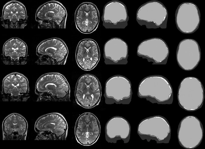
Representative MR slices (left panel) and segmentation results (right panel) for the four subjects (numbering ascending from top to bottom). Color coding of segmentation: dark gray—skin, mid gray—compact skull tissue, white—spongy skull tissue, light gray—interior of skull (CSF, brain gray and white matter, etc.).

All EEG forward computations were performed using the finite element method (FEM). In the current study, hexahedral finite elements of 1 mm edge length were generated using the SimBio‐VGRID FE meshing tool [SimBio, 2009]. To alleviate the effects of the problematic stair‐like approximation of curved tissue boundaries by means of regular hexahedra, a geometry‐adaptation step (node shifting) was applied to smoothen the FE mesh at tissue boundaries [Wolters et al., 2007a]. Although adaptive mesh generation techniques like tetrahedralization approaches [Buchner et al., 1997; Drechsler et al., 2009; Marin et al., 1998; Wolters et al., 2007b] form a possible alternative, their advantage in accuracy when compared to the chosen isoparametric 1 mm geometry‐adapted hexahedral FE approach appeared to be small in previous studies [Lanfer, 2007; Wolters et al., 2007b] and is outweighed by the easy generation and handling of the geometry‐conforming hexahedral meshes.

Besides the special treatment of the skull compartment, all other tissues received isotropic conductivities (Table I). The EEG electrode positions (118 electrodes) were taken from a real neurophysiological experiment and registered afterwards to the volume conductor by using fiducial points.

Table I.

Conductivities of the reference volume conductor [Akhtari et al., 2002; Fuchs et al., 2007; Ramon et al., 2006]

Head tissue	Isotropic conductivity (S/m)
Skin	0.43
Compact bone	0.0064
Spongy bone	0.02865
Brain	0.33

FEM‐Based Forward Modeling

The relationship between bioelectric surface potentials and current sources can be represented by the quasi‐static Maxwell equations with a homogeneous Neumann boundary condition at the head surface [Sarvas, 1987]. Primary current sources are considered as mathematical dipoles [Murakami and Okada, 2006; Sarvas, 1987] and, for a given current dipole and volume conductor, existence and uniqueness for the resulting potential distribution has been proved by Wolters and colleagues [2007b]. In the literature, three different FE methods exist for modeling the mathematical dipole and solving the bioelectric forward problem: the subtraction approach [van den Broek et al., 1998a; Wolters et al., 2007b], the partial integration approach (Awada et al., 1997; Weinstein et al., 2000] and the Venant approach [Buchner et al., 1997]. In this study, we used the Venant approach, a choice, which was based on the comparison between the performances of all three source modeling approaches in multilayer sphere models, which suggested that for sufficiently regular meshes, it yields suitable accuracy over all realistic source locations [Lew et al., 2009b; Wolters et al., 2007a].

The chosen approach has the additional advantage of high computational efficiency when used in combination with the FE transfer matrix approach [Wolters et al., 2004]. An isoparametric FE approach [Braess, 2007; Wolters et al., 2007a] was used to enable the modeling of the geometry‐adapted (deformed) tissue boundary hexahedra as described in the previous section. This FE approach had been validated in a four‐compartment spherical volume conductor and shown to reduce topography and magnitude errors by more than a factor of 2 (1.5) for tangential (radial) sources when compared to a regular hexahedral FE approach [Wolters et al., 2007a]. If S is the number of EEG‐sensors, the FE forward problem using the fast transfer matrix approach [Wolters et al., 2004] leads to (S− 1) large sparse linear equation systems that have to be solved to compute the EEG transfer matrix. We therefore used the incomplete‐Cholesky without fill‐in [IC(0)] preconditioned conjugate gradient [IC(0)‐CG] iterative solver approach, which is implemented in the SimBio‐code [SimBio, 2009] and which features the best balance between computational speed and memory requirements for the investigation in our highly resolved FE head models [see also Lew et al., 2009b]. In our simulation study, the forward problem then had to be solved millions of times. By using the fast transfer matrix approach [Wolters et al., 2004], the computational load could be reduced tremendously [see also Rullmann et al., 2009]. All forward computations were performed with constant source strength of 100 nAm.

If a source comes very close to a next conductivity discontinuity, numerical errors increase [Lew et al., 2009b; Wolters et al., 2007b]. This phenomenon is well‐known for all FE as well as, for example, boundary element (BE) forward modeling approaches. In [Wolters et al., 2007b], a theoretical reasoning was given for this fact. In the present study, we therefore made sure that investigated sources were not too close to a next conductivity discontinuity to avoid such errors.

For approximating the potential we used linear basis functions. Higher order basis functions generally lead to an increased numerical accuracy, but also increase the computational load [Braess, 2007; Marin et al., 1998]. However, at each conductivity jump, the resulting potential function has to have a sharp bend to make sure that the resulting volume current is continuous. Therefore, as proven by Wolters and colleagues [Wolters, 2007c], the potential function can only be in the Sobolev space H¹. Because of the missing smoothness, the impact of higher order basis functions on the numerical accuracy will be the less pronounced the more conductivity discontinuities are introduced into the model. With regard to a realistic inhomogeneous and anisotropic head volume conductor, we therefore prefer to use high resolution in combination with simple linear basis functions.

Skull Conductivity Modeling

We propose and compare several models for the electrical properties of the skull tissue. For skull conductivities we use the measured conductivity values for spongy and compact bone published by Akhtari and colleagues [2002] as the reference (ground truth) model (IMC model, see below) using separate, realistically shaped homogeneous compartments for the two types of skull tissue. Several simplified models (see below) are compared to this reference with respect to forward and inverse solutions. The parameters of the simplified models (e.g., the anisotropy ratio of the anisotropic model) as well as the source configurations are varied. The following models are examined.

Isotropic multi‐compartment model

This model accounts for spongy and compact portions of the skull separately (see Fig. 1) and is considered as a reference or ground truth. It reflects the three‐layered structure of both skull tissues based on MR image segmentation. The classified tissues receive average conductivity values according to Akhtari and colleagues [2002] and Fuchs and colleagues [2007]:

(1)

Isotropic homogeneous model

For all skull voxels considered, a uniform isotropic conductivity value is applied. A widely used skull isotropic conductivity value is 0.0042 S/m [Buchner et al., 1997; Fuchs et al., 2007; Güllmar et al., 2006; Wolters et al., 2006]. However, the work of Akthari and colleagues [2002], Baysal and Haueisen [2004], Gonçalves and colleagues [2003], Lai and colleagues [2005], Oostendorp and colleagues [2000], and Zhang and colleagues [2006] suggest that the ideal isotropic conductivity might be much higher. We considered a range of conductivities between the values for compact and spongy bone (see above).

Anisotropic homogeneous model

A common approach for mimicking the three‐layered skull structure uses anisotropic conductivity tensors to provide different radial and tangential conductivities [Fuchs et al., 2007; Marin et al., 1998; van den Broek et al., 1998b; Wolters et al., 2006]. For the estimation of the tensor direction, a triangulation (of the outer skull surface) is used. By using ASA (version 2.22, Zanow and Knösche, 2004] we were able to estimate a uniformly sampled outer skull surface triangulation (5,054 nodes and 10,104 triangles). This highly smoothed triangulation was created similar to the approach proposed by Wolters and colleagues [2006]. A normal vector was computed for each triangle. Together with the values for radial and tangential conductivities, it defines the conductivity tensor. On the basis of a three‐layered skull, the radial (tangential) conductivities are approximated by a serial (parallel) connection of three resistors. This leads to the following expressions [Wolters, 2003; p. 72):

(2)

(3)

with σ_rad and σ_tan being the apparent radial and tangential conductivities, σ_spong and σ_comp being the conductivities for the spongy and compact bone, and f being the proportion of spongy bone over the entire skull thickness. The average conductivity values (σ_comp = 0.0064 S/m, σ_spong = 0.02865 S/m) are taken from Akhtari and colleagues [2002] and Fuchs and colleagues [2007], f is varied between zero (no spongy layer) and one (only spongy tissue) and is not location‐dependent (i.e., homogeneous over the whole skull compartment) which justifies the name of this model.

Local anisotropic homogeneous model

The purpose of LAH modeling is to disambiguate the differences between the IMC and AH models into the effects of (1) using anisotropy instead of layering and (2) accounting for local differences in the skull properties in the IMC but not in the AH model. The approach is similar to the AH method, except that the anisotropy ratio is computed separately for each tensor, that is, for each skull location. For this purpose, we have to locally estimate the relative thickness of the spongy layer. Our proposed method is based upon thin radially oriented skull profiles from the outer to the inner skull surface at each location. For each profile, a conductivity tensor is computed, the principal eigenvector of which is oriented along this profile. More specifically, each skull voxel is assigned to one outer skull surface triangle by simple projection. All voxels assigned to the same triangle make up one profile. At 20 equally spaced sample points (i = 1…20) along the profile a local proportion of spongy bone f _i was computed by trilinear interpolation of neighboring voxels. The values were then averaged over the entire profile to obtain a local estimate of the proportion of spongy bone f'. The eigenvalues of the anisotropic conductivity tensor were determined by inserting f' (which is thus now location‐dependent or local) into Eqs. (2) and (3).

Local isotropic homogeneous model

The purpose of LIH modeling is to disambiguate the difference between the IMC and IH models into the effects of (1) using a homogeneous skull instead of layering and (2) accounting for local differences in the skull properties in the IMC but not in the IH model. The model construction is similar to the one of the LAH model, except that a locally isotropic conductivity value was used. This conductivity was taken to be equal to the local radial conductivity of the LAH model, because Vallaghé and Clerc [2009] showed that the effect of the skull conductivity mainly comes from its radial component.

Source Modeling

We evaluated the impact of different skull models onto the EEG forward solution based on single focal sources (dipoles) at different locations and with different orientations. Moreover, we evaluated how skull modeling influences the error in single dipole localization. To avoid local minima, parameterization dependencies and instabilities introduced by classical dipole fit optimization methods, we decided to use a goal function scan (GFS) method [Knösche, 1996]. The GFS uses exhaustive sampling of the goal function, which is quantified by a goodness of fit (GOF) between measured data and model prediction. As the localization error depends on the dipole direction, we considered 162 dipole directions at each dipole position, which were uniformly distributed over the surface of a sphere. We used a 15 mm cubic mesh to distribute the dipole positions in the whole brain compartment. To find the minimum of the goal function, a GFS was performed in a spherical volume centered at the true dipole position (radius 40 mm), discretized by a 1 mm grid. This spherical source space was cropped, so that all grid points were located inside the brain volume. To compare and combine results between subjects, the dipole positions were defined in Subject 1 and then transformed to the other brains by means of non‐linear registration of the T1 images using the LIPSIA‐toolbox [Lohmann et al., 2001].

Simulation Setup

To assess the different skull models, we computed errors with respect to the reference model (IMC) for forward and inverse (source localization) results. The forward error was quantified using the relative difference measure (RDM) and the relative magnitude error (relMAG) [Güllmar et al., 2006; Meijs et al., 1989].

(4)

(5)

In these equations, n is the number of EEG channels, m _i and represent the values generated with the reference and the approximated model in channel i, respectively. Although the RDM mainly reflects differences in the topography of the simulated EEG, the relMAG represents overall differences in magnitude. The localization error was quantified as the absolute value of the Euclidian distance between evaluated and reference solutions. We performed the following analyses:

• 1Generalized errors in forward computation: For all simplified skull models (IH, AH, LAH, and LIH), for all four subjects, and for all dipole positions on a 5 mm grid within the brain compartment (three orthogonal dipoles at each position), we compared the EEG forward solution to the reference solution (IMC model). For the IH model, we additionally varied the skull conductivity from σ_comp = 0.0064 S/m to σ_spong = 0.02865 S/m [Akhtari et al., 2002; Fuchs et al., 2007] and including the standard value 0.0042 S/m, which is often used in the literature [Buchner et al., 1997; Fuchs et al., 2007; Güllmar et al., 2006; Wolters et al., 2006], while for the AH model we fixed σ_comp = 0.0064 S/m and σ_spong = 0.02865 S/m and varied the proportion of the spongy bone between f = 0 (no spongy bone) and f = 1 (spongy bone only). Results were displayed as mean and variance over dipoles.
• 2Errors in forward computation for specific locations: To be more specific with respect to the location of the brain activity, we repeated the analysis of (1) separately for five specific brain areas representing the somato‐motor cortex (mean of one dorsal and one ventral position in each hemisphere), the primary auditory cortices, the primary visual cortices, two hemispherically symmetric positions near the frontal pole, and the thalamus.
• 3Spatial distribution of the forward error: To gain more insight into the spatial distribution of the error, we plotted the error for a particularly bad and a particularly good (according to the analysis steps 1–2) skull modeling option, that is, the IH model for σ = 0.0042 S/m (the standard value from literature) and the LAH model, respectively, over selected MR slices. The values were averaged over dipole orientations and subjects (after non‐linear registration).
• 4Spatial distribution of localization error: For the same models as in analysis step 3, we quantified the localization error for dipoles (averaged over subjects) located on a 15 mm grid within the brain compartment. As described above, we used 162 equally spaced dipole orientations. The results were plotted into MR slices using three‐dimensional glyphs.
• 5Relationship between forward and localization error: Finally, we investigated the relationship between forward error (in particular RDM) and localization error by means of scatter plots and correlation analysis.

RESULTS

Generalized Errors in Forward Computation

The results are summarized in Figure 2. We compared all simplified models to the reference model (IMC) using the RDM and relMAG criteria.

Figure 2.

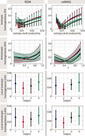
Generalized errors in forward computation. The errors were computed between the respective simplified skull model (IH, AH, LIH, and LAH) and the reference model (IMC). For the IH and AH models, we varied the conductivity and the relative spongy bone proportion, respectively. The colors represent the four different subjects. Results were averaged over all dipoles in the brain. Error bars denote standard deviations. [Color figure can be viewed in the online issue, which is available at wileyonlinelibrary.com.]

For the global methods (IH and AH) both RDM and relMAG curves show a clear minimum, that is, there is an optimal value for the respective varied parameter (conductivity or spongy bone proportion, respectively). Although there is a high degree of consistency, the diagrams also show some inter‐individual differences, most likely related to the varying amount of spongy bone in individual subject skulls. For example, for Subject 3 (black curve), we observe rather high optimal skull conductivity and spongy bone proportion, which is in agreement with the segmentation images (see Fig. 1). It is noteworthy that, for the considered conductivity difference factor of 4.5 and under the condition of optimal parameter choice, the errors do not significantly differ between isotropic and anisotropic models, both for the local and the global cases. On the other hand, the local models perform much better than the global ones. Note, however, that the error curves of the global AH model seem to be less sensitive to the choice of the parameter f (they are at a nearly identically low level for a wide range of f values) than the IH model is to the choice of the isotropic skull conductivity, which might be an advantage with regard to practical applications. In Table II, the optimal parameters for the local models are summarized. It is striking that the optimal conductivity values in the IH model are practically identical to the optimal radial conductivities in the AH model.

Table II.

Optimal parameters for global models

Model	Parameter	Subject 1	Subject 2	Subject 3	Subject 4
AH	f	0.25	0.15	0.65	0.45
	σrad	0.0079 S/m	0.0074 S/m	0.0128 S/m	0.0097 S/m
	σtan	0.0119 S/m	0.0097 S/m	0.0208 S/m	0.0164 S/m
IH	σ	0.0079 S/m	0.0071 S/m	0.0125 S/m	0.0097 S/m

Errors in Forward Computation for Specific Locations

Although the local models provided a very good approximation of the reference model, the global ones produce considerable errors. Therefore, we repeated the analysis for a number of specific brain areas highlight regional differences. The results are depicted in Figure 3.

Figure 3.

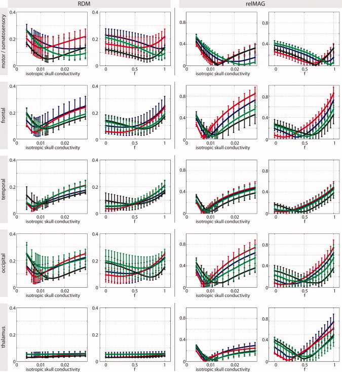
Errors in forward computation for specific brain areas (global models only). The errors were computed between the respective simplified skull model (IH and AH) and the reference model (IMC). We varied the conductivity and the relative spongy bone proportion, respectively. The colors represent the four different subjects. Error bars denote standard deviations. [Color figure can be viewed in the online issue, which is available at wileyonlinelibrary.com.]

For the IH model, it turns out that there are strong differences concerning the optimal skull conductivity. For example, for the somato‐motor areas, which are located near skull sections with a relatively large proportion of spongy tissue (see Fig. 1), the optimal value is much higher than for other brain areas. Moreover, the variability between brain regions differs between subjects. For example, Subject 2 (red curves) shows much more agreement between brain regions than the other subjects. In all cases, however, the optimal conductivity was found to be much higher than the commonly used value of 0.0042 S/m.

A similar statement can be made for the AH model, where the optimal spongy bone proportion differs greatly between subjects and brain areas.

Note that for deep sources such as in the thalamus, the RDM measure is no longer specific, thus rendering the respective curves in Figure 3 rather flat, while inaccurate skull modeling still influences the relMAG measure quite significantly.

To indicate in more detail how the errors are spatially distributed, we mapped them onto selected MRI slices (see Fig. 4) for both the best available model (LAH) and the IH model with the widely used value of 0.0042 S/m for skull conductivity. The results between the two models are very similar, except for the generally higher error level for the IH model. It turns out that particularly large errors are to be expected in areas near the parietal and occipital parts of the skull. The relMAG seems to be high for dipoles directly underneath large spongy skull compartments, especially in the IH model with the standard conductivity of 0.0042 S/m.

Figure 4.

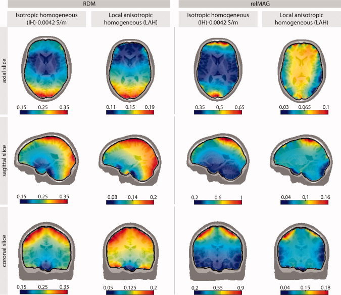
Spatial distribution of average (over all four subjects) forward modeling errors plotted on selected MRI slices of one subject (subject 1). Column 1 depicts the RDM errors of the IH model with the conventionally used skull conductivity value of 0.0042 S/m with respect to the IMC (reference) model. Column 2 shows the RDM error of the LAH model, which in general appeared to be the best approximation of the IMC model (see Fig. 2). Columns 3–4 show the relMAG error, respectively. [Color figure can be viewed in the online issue, which is available at wileyonlinelibrary.com.]

Inverse Analysis

For the IH model, we found localization errors of up to 2 cm, whereas for the LAH model, 6 mm was the upper limit (see Fig. 5a,b). Errors depended a great deal on dipole positions and orientations. In contrast to the RDM and relMAG errors found for the forward solution, the highest localization errors are found in the deeper regions of the brain. For the IH model, the errors are particularly large in parieto‐occipital and cerebellar regions. Although in most regions, the dependence of the error on the dipole orientation is not very strong (round glyphs), however, in the brain stem and cerebellum, the errors are much larger for dipoles pointing in an inferior/posterior to superior/anterior direction. A main reason for this fact might be the sensor coverage, which is especially bad for those sources. For the LAH model, apart from being much smaller, the errors show a more equal distribution throughout the brain. Strong directional dependencies can be found again in the cerebellum.

Figure 5.

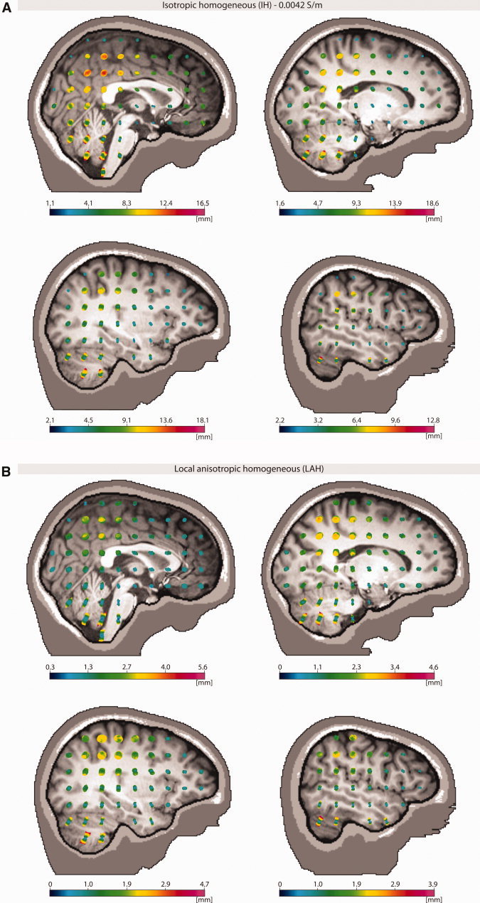
(A) The localization errors are plotted as a function of both dipole position and dipole orientation using glyph plots. For visualization, the glyph is color‐coded with the localization error. We analyzed these models which, for the forward solutions, turned out to be worst (largest difference with reference model), that is the IH (isotropic homogeneous, with conductivity 0.0042 S/m). (B) The localization errors are plotted as a function of both dipole position and dipole orientation using glyph plots. For visualization, the glyph is color‐coded with the localization error. We analyzed these models which, for the forward solutions, turned out to be best (closest agreement with reference model), that is the LAH (local anisotropic) model. [Color figure can be viewed in the online issue, which is available at wileyonlinelibrary.com.]

When comparing the distributions of forward and inverse errors, an interesting question arises: How well does RDM predict localization error? In Figure 6 we plotted RDM versus localization error. Although the graphs show no unique relationship, there is undeniably a certain correlation. In particular, upper and lower limits for the localization error seem to exist, which are linear functions of the RDM. For example, an RDM of 0.025 predicts maximum localization errors between 8 and 10 mm, whereas a RDM of 0.25 predicts minimum localization errors of about 2 mm. The diagrams in Figure 6 also show that local models perform best (blue), the global models with optimized parameters (i.e., at the minima of the curves in Fig. 3) second best (green), and the commonly used IH model with skull conductivity of 0.0042 S/m worst (red).

Figure 6.

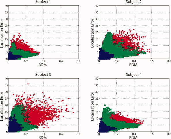
Forward topography error (RDM) and inverse (localization) error interaction depicted individually for each subject. The local models are depicted as blue dots. The optimized models and the standard model (IH, 0.0042 S/m) are shown as green circles and red crosses, respectively. [Color figure can be viewed in the online issue, which is available at wileyonlinelibrary.com.]

DISCUSSION

In this study, we used computer simulations to quantify errors introduced by simplified models of the skull in EEG head modeling. The main goal was to investigate, how well the assumption of anisotropic bone conductivity can approximate the real layered structure of the skull for different source locations and orientations. Moreover, we sought answers to the question what the optimal parameters of the tested models are and how consistent these optima are across source location/orientation and individuals. Finally, we investigated how sensitive the model performance is towards these parameters. To quantify the model performance, we compared forward solutions (i.e., simulated EEG) as well as localization results (i.e., dipole locations and orientations) for the models under investigation with those computed with a reference model. In this reference model (IMC), the different bone tissue compartments (i.e., spongy and compact bone) were modeled explicitly. Because this model is of course an approximation in itself, the obtained errors have to be considered as lower bounds of the actual errors caused by skull modeling. From our results it should become clear, whether and under what circumstances it is sensible to use any of the investigated approaches to account for the material properties of the skull.

The models treated in our work can be divided into local models, where each location on the skull is modeled differently, and global models, where the entire skull is assumed to be homogeneous. The global models represent approaches that have been proposed earlier in the literature. The isotropic homogeneous (IH) model is the one used in the vast majority of studies in conjunction with the analytic sphere model [e.g., Buchner et al., 1995], the boundary element method1 [e.g., Fuchs et al., 2007; Hämäläinen et al., 1993; Kybic et al., 2005], and also the finite element method (Bertrand et al., 1991; van den Broek et al., 1998a; Wolters et al., 2006]. The anisotropic homogeneous (AH) model has been proposed by some authors as an alternative to better account for the layering of the skull [Bertrand et al., 1991; Chauveau et al., 2004; Fuchs et al., 2007; Marin et al., 1998; Rullmann et al., 2009; van den Broek et al., 1998a; Wolters et al., 2006]. Both models deviate from the real structure of the skull in two ways: (1) they assume that the properties of the skull are the same at every location and (2) they approximate the layered skull structure by assuming a single isotropic or anisotropic compartment, respectively. Therefore, in an attempt to disambiguate these influences, we introduced two local models: the local isotropic homogeneous (LIH) and the local anisotropic homogeneous (LAH) model, where only the second factor is present, that is, at each skull location the layered structure of the bone is accounted for by a single (isotropic or anisotropic) conductivity tensor.

For the global models, it turns out that they cause large errors (RDM up to 0.15 and single source localization errors up to 2 cm), even for optimized model parameters (i.e., the conductivity, for IH, and the proportion of spongy bone, which specifies the anisotropy ratio, for AH). In our investigation with the difference factor of 4.5 between the conductivities of spongiosa and compacta [Akhtari et al., 2002; Fuchs et al., 2007], besides being less sensitive to an optimal choice of the free parameter, there was no further advantage of using anisotropy (i.e., AH vs. IH). Furthermore, the values for the optimal model parameters depended heavily on the location of the source (i.e., if the model is optimized for one source location, it can perform very poorly for another one; see Fig. 3). The IH model performance was more sensitive towards the model parameter. In particular, using it together with the widely used skull conductivity value of 0.0042 S/m almost always leads to much higher errors as compared to the respective optimized IH model. To summarize, the results for the global models lead to the following conclusions: (1) the errors introduced using global models are considerable and will vary with source location and orientation, no matter what model parameters are used, (2) for the investigated conductivity difference factor of 4.5 [Akhtari et al., 2002; Fuchs et al., 2007], the modeling of skull conductivity anisotropy with an optimal ratio of just 1:1.6 does not seem to be important, (3) the widely used isotropic conductivity value of 0.0042 S/m seems to be far too small and generally leads to inferior results. Note, however, that the two last statements rest on the assumption that the assumed conductivities for spongy and compact bones, which were derived from the measurements by Akhtari and colleagues [2002], are reasonably accurate. See below for a more detailed discussion of this issue.

Now, we will try to answer the question of, whether the relatively poor performance of the global models was due to the approximation of the layered skull structure by a single conductivity (scalar or tensor) or due to neglecting the differences between different skull locations. It turns out that using the local models, the errors are much smaller and within acceptable bounds (RDM less than 0.06, and localization error less than 4 mm, and for most sources much smaller). Again, in our simulations and for the factor of 4.5, there was no significant advantage of using anisotropy; LAH and LIH nearly performed equally well.

When seeking an answer to the question why the use of anisotropy yields no significant improvement, it is helpful to compare the optimized conductivities of the IH and AH models (Table II). It turns out that the optimal radial conductivity in the AH model is identical to the optimal isotropic conductivity in the IH model. This seems to indicate that the radial skull conductivity is fairly dominant compared to the tangential one.

In conclusion, modeling the local variation of the skull is important, while in our simulations the use of anisotropy for accounting for the layering did not yield a significant improvement. However, for the estimation of the local conductivity one needs to know the local proportion of spongy bone. Knowing this, one may, of course, use the IMC model (here, the reference model) directly.

Needless to say, our approach is also subject to some limitations, which will be discussed in the following. A fundamental as well as inevitable limitation lies in the fact that the “ground truth” is represented by a simplified model as well. The IMC model assumes that the skull is composed of only two different tissue types, that MR images allow a correct separation between these tissues and that the isotropic conductivity values of these tissues are correctly reflected by the measurements of Akhtari and colleagues [2002]. The accuracy of the separation of the different compartments is limited by the finite voxel resolution. We used a typical voxel size of 1 × 1 × 1 mm, which is not insignificant compared to the skull thickness ranging between about 3 and 8 mm. Especially, in thin sections of the skull, partial volume effects are expected to play a role (see also Methods section). Another limitation is the fact that the intensity distributions for spongy and compact bone in MR images do have some overlap. The conductivity values for spongy and compact bone are, most probably, quite variable within and across individuals. Consider, for example, the work of Tang and colleagues [2008], who measured the radial resistivity for a large number of skull samples. They plot their measured resistivity values against the proportion of spongy bone (in our work: f) and find a linear relationship with negative slope, which is in agreement with the prediction from Eq. (2). However, the comparison with Eq. (2) also shows that these values must be biased in some way, as the curve would predict a negative resistivity for (hypothetical) skull segment consisting of spongy bone only (f = 1). Nevertheless, their data seem to suggest a higher ratio between the conductivities of spongy and compact bone than the average values found by Akhtari and colleagues [2002] and used here (about 4.5:1). A factor of more than 8 between spongy and compact bone tissues would for example, have resulted if we had taken the measurement sample with the maximum conductivity difference of Akhtari et al. [2002; see their Table I, sample one, side a). In such cases, the situation might be different and we might also see some difference between the performances of isotropic and anisotropic modeling. In consequence, the scarcity of real measurements of skull conductivity in the literature causes some uncertainty. More work in this direction would certainly allow for an even more precise evaluation of skull models. Free skull modeling parameters might to a certain extent be estimated from individual measurements using the principles of electrical impedance tomography (EIT) as shown by Gonçalves and colleagues [2003] or using a combined analysis of evoked potential/field data as proposed by Baysal and Haueisen [2004], Gonçalves and colleagues [2003], and Lew and colleagues [2009a].

Despite our finding that the use of anisotropy does not seem to be very promising, it might be interesting to compare the optimal anisotropy ratio in our study with recommendations from the literature. In an early study comparing a skull phantom with an analytical concentric spheres model, Rush and Driscoll [1968] estimated an anisotropy ratio of about 1:10. In a more recent work, Sadleir and Argibay [2007] reported that the skull anisotropy ratio must be much smaller than that. On the basis of comparisons with a compartment model (IMC model) using empirical average conductivity values for spongy and compact bone found by Akhtari and colleagues [2002], we identified optimal anisotropy ratios between 1:1.3 and 1:1.7, thus confirming the conclusion of Sadleir and Argibay [2007]. A similar result was also reached by Fuchs and colleagues [2007], based on the same measurements, but assuming a uniform proportion of spongy bone of 1/3.

Given that the isotropic homogeneous (IH) model is the most widespread way to account for the material properties of the skull, it is interesting to discuss our results concerning the optimal skull conductivity in relation to skin/brain conductivities in the light of earlier reports. Rush and Driscoll [1968] reported that a concentric spheres model with a conductivity ratio between brain/skin and skull of 1:80 well fitted their measurements with a physical phantom to which currents were injected at the surface. However, they did not systemically investigate this question. Cohen and Cuffin [1983] used simultaneous EEG and MEG measurements to fit the conductivities of a spherical head model and source parameters (i.e., position and orientation of a single dipole), and came up with a ratio for skin:CSF:skull:brain of 80:240:1:80. More recently, Oostendorp and colleagues [2000] directly measured the radial conductivity of a piece of skull of 7 mm thickness and found a value of 0.015 S/m. Unfortunately, these authors did not give any indication of what part of the skull was used. Comparison with the values found by Tang and colleagues [2008] for different types of skull samples suggests that it must have been a piece with about 70% spongy bone (see both diagrams in their Figure 8). Referencing conductivity values for the brain compartment found in literature [Stoy et al., 1982], they conclude that the conductivity ratio is close to 15:1. They also confirmed this value with an in vivo experiment in which current was injected into a human head and the scalp potential distribution was measured. These data were then used to fit the conductivity values for skin/brain and skull. However, since this procedure involves an ill‐posed problem (only a small fraction of the current actually penetrates the skull) it is unclear, how reliable the result is.

In our study, for the IC model, we find optimal scalar conductivities between 0.007 and 0.013. This is close to the value reported by Oostendorp and colleagues [2000]. Since, however, we used different values for the conductivities of skin and brain, our conductivity ratio is also bigger (25:1–47:1). Therefore, although there is no final answer to the question of the correct conductivity ratio, our study seems to confirm the final conclusion of Oostendorp and colleagues [2000] that the commonly used ratio of 80:1:80 is unrealistic.

CONCLUSIONS

We investigated various ways to model the layered structure of the skull in electroencephalographic forward modeling of the human head, based on the FEM. Our results show that accounting for the local variations over the surface of the skull (inhomogeneity modeling) is important, whereas the use of anisotropy for accounting for the layering does not yield a significant improvement, at least not with the assumed ratio between the spongy and compact bone conductivities of 4.5:1. Moreover, we show that, if using an isotropic and homogeneous skull model, the skull conductivity should be assumed to be higher than the commonly used value of 0.0042 S/m. Our study suggests a skull conductivity of around 0.01 S/m, which corresponds to a conductivity ratio skin:skull:brain of about 40:1:40.

In consequence, we recommend the following ways to model the skull: (1) if the two different tissue types (compact and spongy bone) can be identified (e.g., from MRI) with sufficient accuracy and their conductivity values can be assumed to be known (e.g., from measurements) or can be estimated individually, one should model these explicitly by assigning each skull voxel to one of the two conductivity values, (2) Global models: if the conditions of (1) are not met, one should model the skull as either homogeneous and isotropic, but use a considerably higher skull conductivity than the usually taken 0.0042 S/m (for the four subjects we investigated, we found an average conductivity of 0.0093 S/m) or as homogeneous and anisotropic, but use a considerably higher radial skull conductivity than the usually taken 0.0042 S/m and a considerably lower radial:tangential conductivity anisotropy than the usually taken 1:10 (we recommend a radial:tangential conductivity anisotropy of 0.0093 S/m : 0.015 S/m).

REFERENCES

- Akhtari M, Bryant HC, Marnelak AN, Flynn ER, Heller L, Shih JJ, Mandelkern M, Matlachov A, Ranken DM, Best ED, DiMauro MA, Lee RR, Sutherling WW ( 2002): Conductivities of three‐layer live human skull. Brain Topography 14: 151–167. [DOI] [PubMed] [Google Scholar]
- Awada KA, Jackson DR, Williams JT, Wilton DR, Baumann SB, Papanicolaou AC ( 1997): Computational aspects of finite element modeling in EEG source localization. IEEE Trans Biomed Eng 44: 736–752. [DOI] [PubMed] [Google Scholar]
- Baysal U, Haueisen J ( 2004): Use of a priori information in estimating tissue resistivities—Application to human data in vivo. Physiol Meas 25: 737–748. [DOI] [PubMed] [Google Scholar]
- Bertrand O (1991): 3D Finite element method in brain electrical activity studies. In Nenonen J, Rajala HM, Katila T. (Eds.) (1991): Biomegnetic localization and 3D Modeling, pp. 154–171, Helsinki University of Technology, Helsinki, Finnland. [Google Scholar]
- Braess D (2007): Finite Elements: Theory, Fast Solvers, and Applications in Solid Mechanics, Cambridge University Press; 3 edition (April 30, 2007), ISBN‐10: 0521705185, ISBN‐13: 978‐0521705189. [Google Scholar]
- Buchner H, Adams L, Müller A, Ludwig I, Knepper A, Thron A, Niemann K, Scherg M ( 1995): Somatotopy of human hand somatosensory cortex revealed by dipole source analysis of early somatosensory‐evoked potentials and 3d‐nmr tomography. Evoked Potentials‐Electroencephalography Clin Neurophysiol 96: 121–134. [DOI] [PubMed] [Google Scholar]
- Buchner H, Knoll G, Fuchs M, Rienacker A, Beckmann R, Wagner M, Silny J, Pesch J ( 1997): Inverse localization of electric dipole current sources in finite element models of the human head. Electroencephalography Clin Neurophysiol 102: 267–278. [DOI] [PubMed] [Google Scholar]
- Chauveau N, Franceries X, Doyon B, Rigaud B, Morucci JP, Celsis P ( 2004): Effects of skull thickness, anisotropy, and inhomogeneity on forward EEG/ERP computations using a spherical three‐dimensional resistor mesh model. Hum Brain Map 21: 86–97. [DOI] [PMC free article] [PubMed] [Google Scholar]
- Cohen D, Cuffin BN ( 1983): Demonstration of useful differences between magnetoencephalogram and electroencephalogram. Electroencephalography Clin Neurophysiol 56: 38–51. [DOI] [PubMed] [Google Scholar]
- Cuffin BN ( 1990): Effects of head shape on EEGs and MEGs. IEEE Trans Biomed Eng 37: 44–52. [DOI] [PubMed] [Google Scholar]
- Drechsler F, Wolters CH, Dierkes T, Si H, Grasedyck L ( 2009): A full subtraction approach for finite element method based source analysis using constrained Delaunay tetrahedralisation. NeuroImage 46: 1055–1065. [DOI] [PubMed] [Google Scholar]
- Ellenrieder Nv, Muravchik CH, Nehorai A ( 2006): Effects of geometric head model perturbations on the eeg forward and inverse problems. IEEE Trans Biomed Engm 53: 9. [DOI] [PubMed] [Google Scholar]
- Fuchs M, Wagner M, Kastner J ( 2007): Development of volume conductor and source models to localize epileptic foci. J Clin Neurophysiol 24: 101–119. [DOI] [PubMed] [Google Scholar]
- Gençer NG, Acar CE ( 2004): Sensitivity of EEG and MEG measurements to tissue conductivity. Phys Med Biol 49: 701–717. [DOI] [PubMed] [Google Scholar]
- Gonçalves SI, Munck JC de, Verbunt JPA, Bijma F, Heethaar RM, da Silva FL ( 2003): In vivo measurement of the brain and skull resistivities using an eit‐based method and realistic models for the head. IEEE Trans Biomed Eng 50: 754–767. [DOI] [PubMed] [Google Scholar]
- Güllmar D, Haueisen J, Eiselt M, Giessler F, Flemming L, Anwander A, Knösche TR, Wolters CH, Dumpelmann M, Tuch DS, Reichenbach JR ( 2006): Influence of anisotropic conductivity on EEG source reconstruction: Investigations in a rabbit model. IEEE Trans Biomed Eng 53: 1841–1850. [DOI] [PubMed] [Google Scholar]
- Hallez H, Vanrumste B, Van Hese P, Delputte S, Lemahieu I ( 2008): Dipole estimation errors due to differences in modeling anisotropic conductivities in realistic head models for EEG source analysis. Phys Med Biol 53: 1877–1894. [DOI] [PubMed] [Google Scholar]
- Hämäläinen M, Hari R, Ilmoniemi RJ, Knuutila J, Lounasmaa OV ( 1993): Magnetoencephalography—theory, instrumentation, and applications to noninvasive studies of the working human brain. Rev Mod Phys 65: 413–497. [Google Scholar]
- Haueisen J, Tuch DS, Ramon C, Schimpf PH, Wedeen VJ, George JS, Belliveau JW ( 2002): The influence of brain tissue anisotropy on human EEG and MEG. NeuroImage 15: 159–166. [DOI] [PubMed] [Google Scholar]
- Hoekema R, Wieneke GH, Leijten FSS, van Veelen CWM, van Rijen PC, Huiskamp GJM, Ansems J, van Huffelen AC ( 2003): Measurement of the conductivity of skull, temporarily removed during epilepsy surgery. Brain Topography 16: 29–38. [DOI] [PubMed] [Google Scholar]
- Knösche TR ( 1996): Solutions of the Neuroelectromagnetic Inverse Problem—An Evaluation Study. Netherlands: University of Twente, Twente. [Google Scholar]
- Kybic J, Clerc M, Abboud T, Faugeras O, Keriven R, Papadopoulo T ( 2005): A common formalism for the integral formulations of the forward EEG problem. IEEE Trans Med Imag 24: 12–28. [DOI] [PubMed] [Google Scholar]
- Lai Y, van Drongelen W, Ding L, Hecox KE, Towle VL, Frim DM, He B ( 2005): Estimation of in vivo human brain‐to‐skull conductivity ratio from simultaneous extra‐ and intra‐cranial electrical potential recordings. Clin Neurophysiol 116: 456–465. [DOI] [PubMed] [Google Scholar]
- Lanfer B ( 2007): Validation and Comparison of Realistic Head Modeling Techniques and Application to Tactile Somatosensory Evoked EEG and MEG Data'. Münster: Westfälische Wilhelms‐Universität, University of Münster. [Google Scholar]
- Law SK ( 1993): Thickness and resistivity variations over the upper surface of the human skull. Brain Topography 6: 99–109. [DOI] [PubMed] [Google Scholar]
- Lew S, Wolters CH, Anwander A, Makeig S, MacLeod RS ( 2009a): Improved EEG source analysis using low‐resolution conductivity estimation in a four‐compartment finite element head model. Hum Brain Map 30: 2862–2878. [DOI] [PMC free article] [PubMed] [Google Scholar]
- Lew S, Wolters CH, Dierkes T, Röer C, MacLeod RS ( 2009b): Accuracy and run‐time comparison for different potential approaches and iterative solvers in finite element method based EEG source analysis. Appl Numer Math 59: 1970–1988. [DOI] [PMC free article] [PubMed] [Google Scholar]
- Lohmann G, Müller K, Bosch V, Mentzel H, Hessler S, Chen L, Zysset S, von Cramon DY ( 2001): LIPSIA—A new software system for the evaluation of functional magnetic resonance images of the human brain. Comput Med Imag Graphics 25: 449–457. [DOI] [PubMed] [Google Scholar]
- Marin G, Guerin C, Baillet S, Garnero L, Meunier G ( 1998): Influence of skull anisotropy for the forward and inverse problem in EEG: Simulation studies using fem on realistic head models. Hum Brain Map 6: 250–269. [DOI] [PMC free article] [PubMed] [Google Scholar]
- Meijs JWH, Weier OW, Peters MJ, Vanoosterom A ( 1989): On the numerical accuracy of the boundary element method. IEEE Trans Biomed Eng 36: 1038–1049. [DOI] [PubMed] [Google Scholar]
- Munck JC, Peters M ( 1993): A fast method to compute the potential in the multi sphere model. IEEE Trans Biomed Eng 40: 1166–1174. [DOI] [PubMed] [Google Scholar]
- Murakami S, Okada Y ( 2006): Contributions of principal neocortical neurons to magnetoencephalography and electroencephalography signals. J Physiol London 575: 925–936. [DOI] [PMC free article] [PubMed] [Google Scholar]
- Oostendorp TF, Delbeke J, Stegeman DF ( 2000): The conductivity of the human skull: Results of in vivo and in vitro measurements. IEEE Trans Biomed Eng 47: 6. [DOI] [PubMed] [Google Scholar]
- Pohlmeier R, Buchner H, Knoll G, Rienäcker A, Beckmann R, Pesch J ( 1997): The influence of skull‐conductivity misspecification on inverse source localization in realistically shaped finite element head models. Brain Topography 9: 157–162. [DOI] [PubMed] [Google Scholar]
- Ramon C, Schimpf PH, Haueisen J ( 2006): Influence of head models on EEG simulations and inverse source localizations. BioMed Eng OnLine 5: 10. [DOI] [PMC free article] [PubMed] [Google Scholar]
- Rullmann M, Anwander A, Dannhauer M, Warfield SK, Duffy FH, Wolters CH ( 2009): EEG source analysis of epileptiform activity using a 1 mm anisotropic hexahedra finite element head model. NeuroImage 44: 399–410. [DOI] [PMC free article] [PubMed] [Google Scholar]
- Rush S, Driscoll DA ( 1968): Current distribution in brain from surface electrodes. Anesth Analg Curr Res 47: 717. [PubMed] [Google Scholar]
- Sadleir RJ, Argibay A ( 2007): Modeling skull electrical properties. Ann Biomed Eng 35: 1699–1712. [DOI] [PMC free article] [PubMed] [Google Scholar]
- Sarvas J ( 1987): Basic mathematical and electromagnetic concepts of the biomagnetic inverse problem. Phys Med Biol 32: 11–22. [DOI] [PubMed] [Google Scholar]
- Schimpf PH, Ramon C, Haueisen J ( 2002): Dipole models for the EEG and MEG. IEEE Trans Biomed Eng 49: 409–418. [DOI] [PubMed] [Google Scholar]
- SimBio DG ( 2009): SimBio: A generic environment for bio‐numerical simulations. Available at: http://www.mrt.uni-jena.de/simbio.
- Smith SM, Jenkinson M, Woolrich MW, Beckmann CF, Behrens TEJ, Johansen‐Berg H, Bannister PR, Luca MD, Drobnjak I, Flitney DE, Niazy R, Saunders J, Vickers J, Zhang Y, Stefano ND, Brady JM, Matthews PM ( 2004): Advances in functional and structural MR image analysis and implementation as FSL. NeuroImage 23: 12. [DOI] [PubMed] [Google Scholar]
- Stoy RD, Foster KR, Schwan HP ( 1982): Dielectric‐properties of mammalian‐tissues from 0.1 to 100 Mhz—A summary of recent data. Phys Med Biol 27: 501–513. [DOI] [PubMed] [Google Scholar]
- Tang C, You FS, Cheng G, Gao DK, Fu F, Yang GS, Dong XZ ( 2008): Correlation between structure and resistivity variations of the live human skull. IEEE Trans Biomed Eng 55: 2286–2292. [DOI] [PubMed] [Google Scholar]
- Vallaghé S, Clerc M ( 2009): A global sensitivity analysis of three‐ and four‐layer EEG conductivity models. IEEE Trans Biomed Eng 56: 988–995. [DOI] [PubMed] [Google Scholar]
- van den Broek SP, Reinders F, Donderwinkel M, Peters MJ ( 1998a): Volume conduction effects in EEG and MEG. Electroencephalography Clin Neurophysiol 106: 522–534. [DOI] [PubMed] [Google Scholar]
- Weinstein D, Zhukov L, Johnson C ( 2000): Lead‐field bases for electroencephalography source imaging. Ann Biomed Eng 28: 1059–1065. [DOI] [PubMed] [Google Scholar]
- Wolters CH (2003): Influence of Tissue Conductivity Inhomogeneity and Anisotropy on EEG/MEG based Source Localization in the Human Brain. No. 39 in MPI Series in Cognitive Neuroscience. MPI of Cognitive Neuroscience Leipzig, ISBN 3‐936816‐11‐5 (also: Leipzig, Univ., Diss., http://dol.uni-leipzig.de).
- Wolters CH, Grasedyck L, Hackbusch W ( 2004): Efficient computation of lead field bases and influence matrix for the FEM‐based EEG and MEG inverse problem. Inverse Problems 20: 1099–1116. [Google Scholar]
- Wolters CH, Anwander A, Tricoche X, Weinstein D, Koch MA, MacLeod RS ( 2006): Influence of tissue conductivity anisotropy on EEG/MEG field and return current computation in a realistic head model: A simulation and visualization study using high‐resolution finite element modeling. NeuroImage 30: 813–826. [DOI] [PubMed] [Google Scholar]
- Wolters CH, Anwander A, Berti G, Hartmann U ( 2007a): Geometry‐adapted hexahedral meshes improve accuracy of finite‐element‐method‐based EEG source analysis. IEEE Trans Biomed Eng 54: 1446–1453. [DOI] [PubMed] [Google Scholar]
- Wolters CH, Köstler H, Möller C, Härdtlein J, Grasedyck L, Hackbusch W ( 2007b): Numerical mathematics of the subtraction method for the modeling of a current dipole in EEG source reconstruction using finite element head models. SIAM J Sci Comput 30: 24–45. [Google Scholar]
- Wolters CH ( 2007c): The finite element method in EEG/MEG source analysis. SIAM News 40. [Google Scholar]
- Zanow F, Knösche TR ( 2004): ASA—Advanced source analysis of continuous and event‐related EEG/MEG signals. Brain Topography 16: 287–290. [DOI] [PubMed] [Google Scholar]
- Zhang YC, van Drongelen W, He B ( 2006): Estimation of in vivo brain‐to‐skull conductivity ratio in humans. Appl Phys Lett 89. [DOI] [PMC free article] [PubMed] [Google Scholar]