

Abstract
As a consequence of neural stimulation the blood oxygenation‐level dependent (BOLD) contrast in gradient‐echo echo‐planar imaging (GE‐EPI) based functional MRI (fMRI) leads to an increased MR signal in activated brain regions. Following this, a BOLD signal undershoot below baseline is generally observed with GE‐EPI. The origin of this undershoot has been the focus of many investigations using fMRI and optical modalities, but the underlying mechanisms remain disputed. Here, we investigate the BOLD undershoot following visual stimulation by using a purely T 2‐weighted fMRI sequence at 1.5 and 3 T. By taking advantage of the field strength dependency of the T 2 BOLD contrast and complete absence of static dephasing effects due to the pure spin echoes, one can draw conclusions about the origin of the BOLD undershoot and test the hypotheses in the literature. We observe a significant undershoot at both field strengths, with constant undershoot‐to‐main response ratio. This provides strong evidence that the undershoot is caused by BOLD changes due to elevated post‐stimulus deoxyhaemoglobin concentration in the small vessels. ‘Delayed vascular compliance’ as suggested by the well‐known Balloon and Windkessel models does not appear capable of explaining the undershoot. Our results also suggest that blood volume changes in arterioles and capillaries, for which there is consistent evidence from optical imaging studies, cannot alone cause the undershoot. This has important implications for models of neurovascular response and provides further support for the decoupling of changes in the rate of oxygen metabolism and blood flow. In addition, we found that an ‘arteriolar balloon’ (delayed arterial compliance) may provide a plausible explanation for the temporal characteristics of the BOLD undershoot. Hum Brain Mapp, 2010. © 2010 Wiley‐Liss, Inc.
Keywords: BOLD fMRI, BOLD undershoot, CBF, CBV, CMRO2, arterial balloon model, FSE, spin‐echo
INTRODUCTION
In gradient‐echo (GE) based functional MRI (fMRI), the positive main blood oxygenation level dependent (BOLD) signal response is typically followed by a period in which the signal falls below baseline after the end of stimulation [Buxton et al., 1998; Chen and Pike, 2009; Frahm et al., 1996, 2008; Jones, 1999; Kwong et al., 1992; Mandeville et al., 1999; Sadaghiani et al., 2009; Yacoub et al., 2006; Zhao et al., 2007]. This post‐stimulus period is commonly referred to as the BOLD post‐stimulus undershoot and can persist up to 1 min after cessation of the stimulus [Frahm et al., 1996]. The BOLD response arises because of a combination of physiological changes upon neuronal activation, namely changes in cerebral blood flow (CBF), cerebral blood volume (CBV) and cerebral metabolic rate of oxygen consumption (CMRO2). Although the existence of the post‐stimulus BOLD undershoot is undisputed, it is far from clear which mechanism or combination of mechanisms causes it; it has even been reported that the appearance of the undershoot may depend on the type of stimulus applied [Sadaghiani et al., 2009]. While one recent study claims that transients in fMRI data may be spurious and caused by activation‐related imaging artefacts without physiological basis [Renvall and Hari, 2009], the very widely accepted interpretation is that like the main BOLD response the undershoot is caused by the interplay of some or all of CBF, CBV and CMRO2. Numerous studies have been performed to investigate the origin of the effect, and there are several models and hypotheses discussed in the literature that provide plausible explanations for it [Buxton et al., 1998; Chen and Pike, 2009; Frahm et al., 1996, 2008; Hoge et al., 1999; Jones, 1999; Lu et al., 2004; Mandeville et al., 1999; Turner and Thomas, 2006; Uludag et al., 2004; Yacoub et al., 2006].
We propose in this study that the models can be tested by performing fMRI experiments with a purely T 2‐weighted (spin echo) MR pulse sequence [Poser and Norris, 2007a] at the two main magnetic field strengths of 1.5 and 3 T. Visual stimulation with flickering checkerboards is applied, which is known to lead to a post‐stimulus BOLD undershoot [Sadaghiani et al., 2009].
There are four contrast mechanisms that contribute to BOLD signal changes, two of which are due to extravascular spin dephasing. When the blood oxygenation changes, this leads to a local field perturbation that extends beyond the vessel boundaries. For larger vessels of radius ≥ 10 μm, the path length of diffusive spin motion is relatively small with respect to the extent of this dipole field, and this process results in extravascular static dephasing, which causes classical T 2*‐weighted signal decay. This static dephasing is refocused in spin echo sequences. Around smaller capillary and post‐capillary vessels (microvasculature), diffusing spins experience a relatively large field variation. The loss of phase coherence hence becomes stochastic and can no longer be refocused by a spin echo; this contrast mechanism is called extravascular dynamic dephasing and constitutes a T 2 effect [Ogawa et al., 1993]. The remaining two contrast mechanisms are of intravascular origin. First, the intravascular frequency offset effect, which arises from an effective field shift inside a vessel, which is dependent upon the angle subtended by the axis of a (presumed) cylindrical vessel and B 0. In a voxel containing many randomly oriented vessels, this effectively behaves like static dephasing and hence a T 2* effect and is invisible in spin‐echo experiments. The second intravascular effect is due to changes in the intravascular T 2 relaxation time, which directly depend on the deoxyhaemoglobin concentration [Kennan et al., 1994]. This effect is spatially relatively unspecific, as it is common to all post‐capillary vessels, and to some extent the capillaries.
The gradient echo experiment is sensitive to all four BOLD mechanisms; however, only intravascular T 2 changes and extravascular dynamic averaging will contribute to the spin echo, and hence the purely T 2‐weighted sequence used in this study. Since extravascular dynamic averaging causes signal changes around micro‐vessels, they are expected to yield a high‐spatial specificity as they originate closer to the site of neuronal activation. At 1.5 T, nearly 100% of the positive spin echo (SE) BOLD signal change is of intravascular origin [Constable et al., 1994; Jones, 1999; van Zijl et al., 1998]. At 3 T, this contribution is reduced to about 50% [Jochimsen et al., 2004; Norris et al., 2002]; the remainder is due to dynamic dephasing in the microvasculature. The increased spatial specificity of T 2‐weighted fMRI with SE‐EPI, when compared with T 2*‐weighted fMRI with GE‐EPI, typically makes SE‐EPI the method of choice for applications on both humans and animals at very high main magnetic field strengths of 7 T and above, and could also be demonstrated in the human at 3 T [Norris et al., 2002; Parkes et al., 2005]. The use of SE‐EPI implies a potentially significant T 2*‐weighting due to the long EPI readout, the degree of which will depend on the spatial frequencies present in the activation area. This can be avoided by the use of pure SE sequences [Constable et al., 1994; Poser and Norris, 2007a], such as a fast spin‐echo sequence.
The field strength dependence of the T 2 contrast can be exploited in a straightforward, yet very robust manner to investigate the origin of the BOLD undershoot: Conclusions can be drawn both from the occurrence of an undershoot, and the ratio of the undershoot to the main BOLD response at the two different field strengths. In the following sections we will first briefly summarise the existing models for the post‐stimulus undershoot and describe how these can be tested.
MODELS FOR THE POST‐STIMULUS BOLD UNDERSHOOT
Delayed Vascular Compliance
One of the most prominent models is the balloon model [Buxton et al., 1998], which is based on data obtained from anaesthetised rats receiving electrical forepaw stimulation. CBV measurements with MION contrast agent showed a slow post‐stimulus return of CBV in comparison to CBF and CMRO2. According to this model, a temporal post‐stimulus decoupling of CBF and CBV causes a relatively slower return of venous CBV to baseline. This is postulated to arise from the vaso‐mechanical properties of the venous vessels: Upon neuronal activation, the local increase in blood flow, and therefore blood pressure, causes vaso‐dilation in the venous bed, which is largely accountable for the rise in CBV during activation. Following cessation of the stimulus, the passive process of re‐contraction lasts longer than the return of CBF back to baseline. This is often referred to as delayed vascular compliance. The consequence is a temporal ‘mismatch’ between CBV and CBF. A similar mechanism for the undershoot was proposed by [Mandeville et al., 1999], based on the same data. The post‐stimulus undershoot was attributed to a ‘post‐capillary Windkessel’ that accommodates an elevated blood volume beyond the period of increased blood flow. Both Balloon and Windkessel models thus interpret the undershoot as a consequence of the mechanical characteristics of the vasculature rather than the physiological or metabolic processes directly associated with the neuronal activation.
It could be shown that the balloon model can be successfully adapted from rodent data [Buxton et al., 1998] to human data at both 1.5 T [Feng et al., 2001; Friston et al., 2000], and 3 T [Mildner et al., 2001; Obata et al., 2004] yielding parameters within physiologically plausible ranges. A modification of the Windkessel model incorporating a delayed compliance was proposed by Kong et al. [2004], to improve the description of the post‐stimulus vaso‐dynamics. The balloon model calculations in [Obata et al., 2004] however show that a substantial variation in the CMRO2 and CBV responses can yield very similar CBF and BOLD responses: a good model fit to the experimental data hence does not necessarily imply that the model is thereby validated given the large number of degrees of freedom associated with it.
Sustained Elevation of CMRO2
A second plausible explanation for the post‐stimulus undershoot is a sustained increase in oxygen consumption after blood flow has returned to baseline. Continued oxygen metabolism after cessation of neuronal activation and at baseline CBF would result in an increase in the amount of deoxyhaemoglobin in the venous capillaries and draining vessels. This mechanism was suggested in early work by Frahm and colleagues [1996]. Evidence that CBV can return to baseline simultaneously with BOLD, and hence by implication CBF, was provided in MION‐weighted cat studies by Harel et al. [2002], and more recently Nagaoka et al. [2006] who investigated CMRO2 changes in the absence of CBV changes under hypotension. MR studies using the recently developed VASO technique [Lu et al., 2003] report similar findings. The first of these [Lu et al., 2004] shows a strong BOLD undershoot after both CBV and CBF have returned to baseline, a result that has since been supported by other VASO studies [Donahue et al., 2008; Gu et al., 2005; Poser and Norris, 2007b]. A VASO study into the undershoot under hypoxic conditions [Tuunanen et al., 2006] demonstrates that CBV is at resting state level during the BOLD undershoot period. In addition, functional bolus tracking experiments revealed the expected change in CBV during the main BOLD response but not during the undershoot [Frahm et al., 2008]. These again support a metabolic rather than haemodynamic mechanism for the undershoot.
Functional near‐infrared spectroscopy (fNIRS) studies [Jasdzewski et al., 2003; Schroeter et al., 2006] reported a decrease in oxyhaemoglobin and increase in deoxyhaemoglobin that accompany the BOLD undershoot; notably, total haemoglobin as a measure of CBV returned to baseline immediately after the end of stimulation. In agreement with this, measurements of tissue oxygen tension showed a clear post‐stimulus pO2 undershoot [Ances et al., 2001], while CBF as measured with laser‐Doppler flowmetry quickly returned to baseline [Ances et al., 2001]. These non‐MR studies thus show that deoxyhaemoglobin remains increased after total haemoglobin (CBV) and oxyhaemoglobin (CBF) has returned to baseline, suggesting an accumulation of deoxyhaemoglobin in the tissue as would be the result of post‐stimulus prolonged oxygen metabolism, rather than a CBV effect.
A mechanism by which CMRO2 remains elevated for a considerable duration post‐stimulus seems physiologically plausible, as oxygen is required to re‐establish ionic concentration gradients that discharge during neuronal activation. This restoration process which is thought to account for most of the brain energy demand [Attwell and Laughlin, 2001] has been shown to last 30–40 s following the offset of stimulation [Brockhaus et al., 1993], in a very good agreement with the typical duration of the BOLD undershoot.
CBV Changes in Capillaries
There is a growing body of evidence that a large proportion, if not all, of the CBV change takes place in the arterioles and capillaries. This is particularly reported in the recent optical imaging literature [Berwick et al., 2005; Devor et al., 2003, 2007; Hillman et al., 2007; Villringer et al., 1994]. These studies report a change in total haemoglobin, and by implication in CBV, in the parenchyma upon activation. Using a novel depth‐resolved (3‐D) optical imaging technique with simultaneous recording of oxy‐, deoxy‐ and total haemoglobin [Hillman et al., 2007] could show significant stimulus‐related increases in parenchymal total haemoglobin concentration that match the observed arteriolar dilation; very small total haemoglobin changes are reported for the venous side, in the absence of measurable venous volume changes. Instead, it appeared that the flow increase in the veins concomitant with arteriolar CBV change manifests itself as a change only in the venous flow speed.
Also in recent animal MR studies by Kim et al., it was observed that the majority of total CBV change upon neuronal activation originates from changes in arterial (and not venous) CBV [Jin and Kim, 2008a, b; Kim et al., 2007). The CBV response to visual stimulation in the human observed by [Wu et al., 2008] slightly leads the BOLD response, indicative of a fast arterial CBV increase while the BOLD signal by its nature originates largely from the vasculature downstream of the site of neuronal activation.
No satisfactory explanation for how the parenchyma can accommodate the observed increases in haemoglobin following arteriolar dilation has to date been proposed in the literature, which is why many models assume an invariant capillary CBV and total haemoglobin [Buxton et al., 1998; Mandeville et al., 1999]. While CBV changes clearly occur somewhere in the vasculature, it is often somewhat carelessly assumed that space for the activation related CBV increase can in some way be found in the brain. The rise in CBV associated with a strong and sustained stimulus, such as visual stimulation, could lead to a pressure increase with fatal consequences if not (at least in part) compensated by a corresponding volume decrease of another compartment [Turner and Thomas, 2006]. These authors proposed a mechanism that could explain how the observed parenchymal CBV changes are physiologically feasible. According to this mechanism, the endothelium of the capillaries acts as an exchange pool from which water molecules can diffuse into the intra‐capillary space, thereby leading to a volume increase of the blood pool without need for a bulk volume change. Although the Turner‐Thomas model does not primarily aim at explaining the BOLD undershoot, it does however incidentally suggest that the undershoot could originate as a CBV effect in the capillaries, where the endothelium accounts for up to 20% of the intra‐capillary space and would then act as an equivalent of the ‘post‐capillary Windkessel’: If the return of the capillary diameter to baseline is driven by osmotic gradients then the time constants associated with it are likely slow and may match the typical order of the BOLD undershoot [Turner and Thomas, 2006]. Furthermore, the CBV recovery in the parenchyma would be expected to last longer than that of CBF (in analogy to the delayed venous compliance), and larger draining vessels should not undergo a volume change. Further downstream, the relative contribution of the single‐layered endothelium to the total vessel volume rapidly drops with increasing vessel diameter, arguing for a very good localisation of the undershoot to the site of neuronal activation.
HYPOTHESES ON MR SIGNAL CHANGES FOR PURELY T 2‐WEIGHTED fMRI
Delayed Vascular Compliance
If the undershoot is the result of a decoupling of CBV and CBF in the downstream vasculature as suggested in the balloon model, then the standard interpretation is that it can be explained by extravascular static dephasing that takes place around the larger draining veins. There would be no intravascular T 2 change as both CBF and CMRO2 will have returned to their baseline values, but a transiently increased CBV in the venous compartment due to the delayed compliance. Static dephasing is exclusively a T 2* effect and hence not visible if a pure SE sequence is used, since then all static dephasing effects are refocused and only the T 2 contrasts remain. For a blood T 2 shorter than that of the surrounding gray matter, an elevated post‐stimulus CBV might cause a small signal reduction especially at 3 T; this however is counteracted by the fact that at 3 T extravascular dynamic dephasing contributes to the main response but not the undershoot, thereby in turn serving to reduce the undershoot to peak ration. At 1.5 T, the T 2 of venous blood is comparable to that of grey matter, and no undershoot can be predicted. Therefore if the delayed vascular compliance model is correct then a very strongly reduced, or absent undershoot should be seen in pure SE data at either field strength.
Sustained Elevation of CMRO2
Continued increased oxygen consumption after the end of stimulation, and the return of both CBV and CBF to baseline would result in an increase in the amount of deoxyhaemoglobin. This would cause a reduction in the intravascular T 2 of blood, and at 3 T an increase in extravascular dynamic dephasing: both mechanisms would contribute to the lower MR signal during the undershoot. The undershoot would thus be a ‘negative’ BOLD effect and arise from the same combination of contrast mechanisms as the main positive BOLD signal change. Hence, an undershoot should also be seen in T 2‐weighted data at both field strengths. While signal changes at 3 T would be expected to be considerably larger than at 1.5 T due to the additional contribution of extravascular dynamic averaging effects, the ratio of main BOLD effect to undershoot should be constant across field strengths.
CBV Changes in Capillaries
If there is no volume change on the venous side and only the capillaries expand upon activation, then once CMRO2 and CBF, and thus venous T 2 have returned to baseline after stimulus cessation, any observed signal contributions to the SE BOLD undershoot would arise from the prolonged volume change in the capillaries, and be due to dynamic averaging, and possibly changes in capillary T 2.
This would lead to the observation of an undershoot in SE BOLD at 3 T. In the absence of additional post‐capillary/venous T 2 changes, the negligible signal contribution from dynamic averaging effects at 1.5 T, however, would lead to a strongly reduced or absent undershoot at 1.5 T. If the ‘collapse’ of the endothelium is the mechanism for the CBV change in accordance with the Turner‐Thomas hypothesis, and its recovery after the cessation of the stimulus results in the implied temporal CBV‐CBF decoupling, then for a MR pulse sequence with only T 2 contrast this implies that dynamic averaging about the capillaries should generate an undershoot at 3 T, but not at 1.5 T.
A post‐stimulus elevated CBV in the capillary bed that persisted after the return of CMRO2 and CBF to baseline would necessarily lead to a local reduction of blood flow velocity in the expanded capillaries. Under the common premise that CMRO2 is the product of blood flow and oxygen extraction fraction (OEF), an increase in OEF would ensue even at baseline CMRO2. The consequence would then be a post‐stimulus accumulation of deoxyhaemoglobin in the capillaries, but not in the post‐capillary vessels. This would lead to an observable undershoot at 3 T; but at 1.5 T the undershoot would be very small and likely negligible since spin echo at 1.5 T would only detect the intravascular contribution from the capillary compartment.
The models and their respective outcomes for the SE BOLD experiments are summarised schematically in Figure 1.
Figure 1.
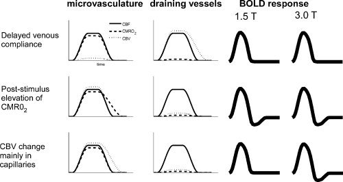
Schematic summary of the CBF, CBV and CMRO2 time courses associated with the different models for the undershoot, and the T 2‐weighted BOLD response that would be expected for each of them at 1.5 and 3 T.
MATERIALS AND METHODS
Experiments were performed on 1.5 T Avanto and 3 T Trio TIM systems (Siemens, Erlangen, Germany), using the product 32‐channel head coils at both field strength. A purely T 2‐weighted HASTE fMRI sequence was used as previously described [Poser and Norris, 2007a]. In short, the sequence refocuses the first spin echo at a TE of 50 ms to allow for dynamic averaging, followed by a rapid, linearly ascending, HASTE readout. The k‐space centre is acquired at the target TE of 80 ms to optimise sensitivity for the dynamic averaging signal. A schematic of the sequence is shown in Figure 2. As grey matter T 2 is similar at both fields, identical acquisition parameters were used. Six slices were acquired with a TR of 2 s and resolution 3.5 × 3.5 × 5 mm3 (matrix size 64 × 64, no slice gap). To shorten the echo train length and reduce power deposition, factor four parallel acceleration with GRAPPA image reconstruction was employed. Fat saturation was used. Each measurement lasted 10 min, yielding 300 data points. For further details see [Poser and Norris, 2007a]. As an additional reference experiment to simultaneously acquire T 2* and T 2‐weighted signal time courses at 3 T, we used a combined dual‐echo GE‐ and SE‐EPI sequence, with TE = 23 and 80 ms, respectively, BW = 1960 Hz/px, 150 time points (5 min scan time), but otherwise identical geometric parameters. The vendor provided ‘AutoAlign’ scan was performed at the beginning of each of the two sessions to ensure identical slice positioning at both field strengths, and to yield the same anatomical coverage for all subjects.
Figure 2.
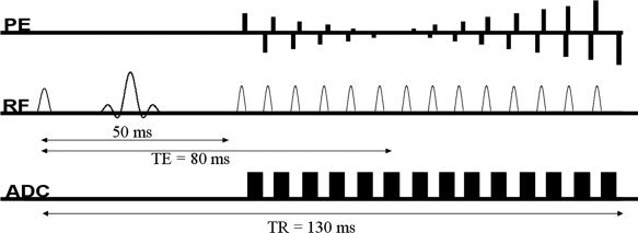
T 2 weighted HASTE fMRI sequence used in this study. To allow dynamic averaging to take place, the preparation experiment forms the first echo at a TE of 50 ms. The k‐space centre is acquired at a TE of 80 ms to maximize functional BOLD contrast.
At each field strength, measurements were made on the same 14 subjects with normal or corrected‐to‐normal vision. Before the start of the experiments, informed consent was obtained in writing according to local regulations. The stimulus consisted of a black‐and‐white flickering checkerboard (frequency 10 Hz), which was presented in blocks of 20 s ‘on’/40 s ‘off’ using VSG (ViSaGe, Cambridge Research Systems, Rochester, England) stimulation equipment, which was controlled using the CRS Toolbox for Matlab. The long rest period was chosen to allow full BOLD signal recovery. Throughout both ‘on’ and ‘off’ blocks, subjects were instructed to maintain fixation on a small cross that underwent random colour changes, to which they had to respond by button presses.
Data pre‐processing and analysis were performed with Brainvoyager 2000 (BrainInnovation, Maastricht, The Netherlands) and custom‐written software implemented in Matlab. Pre‐processing included 3‐D motion correction and removal of linear intensity drifts. No other temporal or spatial smoothing was applied. Two of the 14 subjects were excluded from the analysis due to strong discontinuities in the signal timecourse, apparently caused by abrupt subject motion in the through‐plane direction which was not properly detected nor ‘corrected’ by the 3‐D algorithm due the limited volume coverage in the slice direction. For the remaining subjects, the detected motion was well below one voxel.
For statistical analysis of the T 2‐weighted data, t‐tests were performed on the individual subjects, with the significance threshold set to P < 0.01. Activation time courses were extracted as the average stimulus response of the voxels that met the activation criterion at both static magnetic field strengths. The baseline level was taken as the average signal of the three time points preceding stimulus onset.
The average stimulus response across subjects was calculated as the normalised event‐related average of the individual response curves to ensure equal weighting of each subject. The undershoot‐to‐main response ratio was then determined from the average BOLD response curve, by computing the ratio of the integrals as the ‘area under’ the main response (Intmr) and undershoot response (Intur).
To investigate a possible spatial dependence of the undershoot behaviour, the activated voxels in each subject were sorted according to percent signal change in the positive part of the BOLD response in the pure spin‐echo data. Since the spatial resolution of the fMRI experiment is too limited for a detailed spatial analysis, the 25% of voxels with the highest signal change at 3 T were, as an approximation, taken as voxels where the signal change would be dominated by larger draining vessels. The undershoot‐to‐main response ratio in the group average of these voxels was compared to that of the remaining 75% of voxels, which were assumed to contain mainly tissue. The ‘vessel’ and ‘tissue’ ROIs were obtained at 3 T to include any pixels that might be activated due to dynamic averaging effects, and applied to both datasets so as to consider exactly the same pixels at each field. Furthermore, we investigated whether any changes in undershoot‐to‐peak ratio for the different compartment would be caused by changes of the main response amplitude or the undershoot.
The additional GE‐ and SE‐EPI measurements acquired at 3 T were analysed by performing t‐tests at P < 0.0001; the overlap of the activation maps thus obtained was then used as ROI for both data sets. Again, the resulting individual subject time courses were normalised before averaging.
For comparison of the sensitivity of the sequences at the two field strengths, we calculated the temporal signal‐to‐noise ratio (tSNR) in all subjects, using all 300 time points after motion correction and linear trend removal. An identical ROI of 480 voxels was placed in the frontal brain so as not to be affected by the occipital activation.
RESULTS
The tSNR measurements yielded 39.30 ± 7.77 and 48.57 ± 11.76 at 1.5 and 3 T, respectively (mean ± SD). The tSNR of the sequence at the two fields obtained from the ROI in the frontal brain is hence comparable, although the sensitivity is somewhat higher at 3 T as might be expected.
A pronounced undershoot is clearly observed in the subject average at both field strengths, as can be seen by reference to the left panel of Figure 3. With 1.17 and 1.61% signal changes at 1.5 and 3 T respectively, the average percentage BOLD response is considerably larger at 3 T. This agrees with the expectation of an additional contribution from dynamic averaging effects at the higher field strength.
Figure 3.
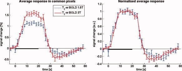
BOLD signal changes at 1.5 and 3 T as measured with pure T 2 contrast, averaged over subjects (N = 12). A post‐stimulus BOLD undershoot is clearly present at both field strengths. The average percent signal change at 1.5 T (1.17%) is much lower than at 3 T (1.61%), as would be expected because of the additional contribution of dynamic averaging effects at the higher field strength. The panel and the right shows the normalised T 2‐weighted BOLD response curves overlaid, illustrating the essentially identical time course at both fields. In the individual subject response curves baseline was taken as the average of the 5 s proceeding stimulus onset; the individual curves were then normalised prior to averaging to ensure equal weighting. Error bars show SEM over subjects. The 20‐s stimulation period is indicated by the solid black line on the time axis. [Color figure can be viewed in the online issue, which is available at wileyonlinelibrary.com.]
The undershoot‐to‐main response ratio (ratiour/mr) at 1.5 and 3 T is 0.20 ± 0.09 and 0.22 ± 0.07, respectively. Here, the error in the ratio (σratio) was calculated as σratio/ratiour/mr = [(σmr/Intmr)2 + (σur/Intur)2]1/2, where σmr and σur are additional integral increments obtained by including the SEM on each point in the curves in the integral calculation for the main response (mr) and the undershoot (ur) respectively. The normalised timecourses are shown in the right panel of Figure 3, which illustrates clearly that the signal timecourses have essentially identical characteristics at both field strengths. Moreover, the GE‐ and SE‐EPI data that were acquired with the double echo sequence at 3 T also show an identical timecourse behaviour (Fig. 4), in the ROI defined by the commonly activated voxels (P < 0.001). Since simultaneous acquisition was used, very reliable quantitative comparisons can be made, despite the fact that some degree of T 2*‐weighting can be expected also in the SE‐EPI data.
Figure 4.
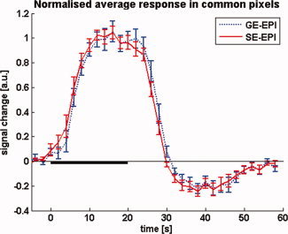
Average normalized stimulus response curves as simultaneously measured at 3 T using the double echo GE‐ and SE‐EPI sequence. No difference in temporal characteristics is observed between the two methods. [Color figure can be viewed in the online issue, which is available at wileyonlinelibrary.com.]
The comparison of undershoot‐to‐main response ratio in ‘vessel’ versus ‘tissue’ voxels at 1.5 T yields an undershoot‐to‐main response ratio of 0.12 ± 0.06 and 0.23 ± 0.07 for ‘vessel’ and ‘tissue’ voxels, respectively. At 3 T, the corresponding ratios are 0.10 ± 0.04 and 0.26 ± 0.04, respectively. The corresponding signal timecourses are shown in Figure 5. Clusters of ‘vessel’ voxels are found particularly near the sagittal sinus and the cortical surface as would be expected. An example for the segmentation of ‘tissue’ and ‘vessels’ for one subject is shown in Figure 6. Plotting the positive percentage signal change of all considered pixels (pooled over subjects) in histograms reveals a nearly identical distribution at 1.5 and 3 T (see online supplementary Fig. 1).
Figure 5.
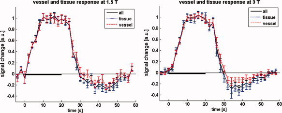
Average normalised stimulus response for the different compartments at 1.5 and 3 T, separated on the basis of signal change. Timecourses for the ‘tissue’ and ‘vessel’ voxels are shown in blue and red, respectively. The solid black curves show the average over all active voxels. [Color figure can be viewed in the online issue, which is available at wileyonlinelibrary.com.]
Figure 6.
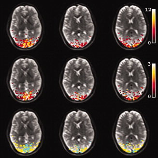
Example of activation maps from one subject at 3 T, overlaid on three slices of the corresponding T 2‐weighted HASTE images (top row). Also shown are the percent signal changes (middle row), and the vessel‐tissue segmentation map (bottom row). For the latter, active voxels were subdivided into ‘tissue’ and ‘vessel’ voxels by sorting them according to positive percent signal change. The top 25% were considered voxels with a large contribution from draining vessels, depicted in green. The remaining 75% were taken as tissue voxels, depicted in yellow.
When changing the threshold so as to separate out much less than 25% of voxels, an increasing tendency is observed that indicates a reduced undershoot‐to‐main response ratio for the voxels exhibiting the largest signal change. This tendency appears to be more pronounced at 3 T than 1.5. Interestingly, the change of the undershoot‐to‐main response ratio is caused by a relatively larger positive BOLD response while the percentage signal change of the undershoot is nearly invariant at both fields. The reader is referred to Figures 2 and 3 in the online supplementary material which show the percentage change time courses for a stricter vessel‐tissue separation (5–95%), and scatter plots of percentage undershoot vs. percentage main response; the latter provide a good illustration of the constancy of the undershoot while the main response varies.
DISCUSSION
No generally accepted consensus has been reached in the literature as to what causes the BOLD post‐stimulus undershoot, in part because the haemodynamics within the different vascular compartments remain disputed. We propose here that the origin of the undershoot can be pinpointed by using fMRI with pure T 2 contrast.
We observed a pronounced BOLD undershoot in the T 2‐weighted data at both 1.5 and 3 T. The temporal characteristics and ratios of main BOLD‐response to undershoot are very similar. This points towards a BOLD mechanism for the undershoot in which exactly the same combination of contrast mechanisms is active during the main and undershoot BOLD responses. In further support of this, we observed no difference in the temporal characteristics and undershoot‐to‐main response ratio of GE‐ and SE‐EPI BOLD responses at 3 T, implying that T 2 and T 2* contrasts give identical BOLD response curves with regard to these parameters. A clear BOLD undershoot in SE‐EPI can also be seen at 1.5 T, as is, for instance evident from the work of [Jones, 1999]; albeit this may also in part be attributable to residual T 2* contributions.
The fact that the shape of the BOLD response curves does not change as a function of field strength, despite the differing contrast mechanisms that contribute to the signal, leads to the conclusion that the measured curves are proportional to the time course of deoxyhaemoglobin content.
Looking into a possible dependence of the undershoot on the venous volume revealed that the undershoot‐to‐peak ratio for each compartment is not significantly different at both field strengths. At the spatial resolution of typical fMRI on which our interest is focused, however, a detailed separation of voxels by tissue and vessel content is clearly only approximate. We therefore chose an approximation by which voxels were rated according to the (positive) BOLD signal change. For an increasingly smaller fraction of voxels with the largest vessels, there is a tendency towards a reduced undershoot‐to‐main response ratio. Clearly, the vast majority of voxels did show a post‐stimulus undershoot, independent of the field strength used. Moreover, this undershoot is nearly constant for all active voxels, and the undershoot‐to‐main response ratio is determined by the amplitude of the positive portion of the BOLD response.
It should be concluded from our observations that the undershoot arises due to changes in the amount of intravascular deoxyhaemoglobin, and not a temporal CBV‐CBF decoupling. If the undershoot seen in GE‐EPI were solely caused by the vaso‐mechanical effects postulated by the Balloon and Windkessel models, the undershoot should have been absent in the pure spin‐echo data.
If one considers parenchymal CBV changes, for instance by the mechanism of endothelial water exchange described by Turner and Thomas, then a more pronounced undershoot compared with 1.5 T should have been seen at 3 T as a result of dynamic averaging about the microvasculature. At 1.5 T, the absence of a contribution of dynamic averaging effects would have resulted in the observation of no (or a strongly reduced) undershoot.
Our findings thus provide evidence for an increased deoxyhaemoglobin level even after the return of CBV and CBF to baseline.
Increased post‐stimulus deoxyhaemoglobin levels are consistent with the notion of continued elevation in oxygen metabolism as concluded by other authors [Donahue et al., 2008; Lu et al., 2004], based on MR experiments that were aimed at directly but separately measuring the different physiological parameters GE‐BOLD, CBV and CBF. Such an approach clearly has the advantage that each parameter can be studied separately, but requires the combination of data acquired with methods of differing sensitivity. Using an entirely different approach with only a single type of MR pulse sequence we have been able to draw the same conclusion. Our observations are also consistent with the recent MR findings from Frahm et al.'s [2008] bolus‐tracking fMRI experiments.
Previous data were obtained at a field strength of 1.5 T, thus without being sensitive to the BOLD contribution of extravascular dynamic averaging around the capillaries; in our experiments at 3 T we assume that 50% of the signal originates from the microvasculature [Jochimsen et al., 2004; Norris et al., 2002], allowing estimation of the capillary contributions. Another study however has implied that the difference in signal sources between 1.5 and 3 T may be smaller than that [Duong et al., 2003], suggesting that measurements at an additional higher field strength such as 7 T would have allowed to address the experimental question with more certainty than was possible here: with increasing field strength the dominant relative contribution to the BOLD signal shifts from the intravascular (blood) compartment towards the smaller vessels (venules and arterioles) and capillaries. The application of small diffusion‐weighting gradients in the sequence to take advantage of any flow differences between the different intravascular compartments, such as arterioles and venules [Duong and Kim, 2000; Lee et al., 2001] could also be considered in future studies even though this may in practice turn out to be challenging in the human due to limited SNR.
One shortcoming of the present study is the relatively low spatial resolution. While typical for human fMRI studies, the resolution used here is insufficient to discern a possible spatial dependence of the BOLD undershoot, as has been proposed by Yacoub and colleagues [2006] on the basis of high resolution cat data acquired at 9.4 T. Jin and Kim [2008a] find an undershoot in rat data for both BOLD, CBF and CBV whereby the CBV‐CBF coupling is spatially dependent; this also points towards a possible spatial dependence of the undershoot. In the human such resolutions are unfeasible to achieve, and an implicit assumption of this study is hence that the undershoot can be explained by one dominant mechanism. That multiple mechanisms are active cannot be ruled out entirely.
Another potential source of criticism is the choice of echo time for the spin‐echo BOLD measurements. We here chose a TE of 80 ms at both 1.5 and 3 T as this is close to the grey matter T 2 value at both fields, and the capillary gray matter compartment is clearly the most interesting in an fMRI context. However since the intravascular blood T 2 is more strongly field strength dependent this might introduce some bias as the relative contribution of the blood compartment differs across field strengths. For the reason given, however, the choice of 80 ms for both protocols seemed to be the more obvious compromise.
A possible theory for the BOLD undershoot that was not investigated here is a post‐stimulus undershoot in CBF, which at both field strengths would be expected to result in a BOLD undershoot, with or without post‐stimulus elevation in oxygen uptake. At least during the undershoot period, CMRO2 and CBF are likely decoupled from each other, but this does not necessarily imply that one parameter returns to baseline first, and for weak or brief stimuli they might return at the same time. If CMRO2 were to return before CBF one would expect a biphasic response with no undershoot. While the occurrence of a CBF undershoot would clearly provide a direct explanation for the undershoot in the corresponding BOLD signal [Frahm et al., 1996; Friston et al., 2000; Hoge et al., 1999; Shmuel et al., 2006; Uludag et al., 2004], it has so far not been widely reported in the abundant ASL literature. One early account was given by Hoge and colleagues [1999], later supported by Shmuel et al. [2006], and more recently a human fMRI study into the BOLD undershoot that supports the delayed venous compliance model but incidentally also finds a possible significant, but nevertheless very small contribution of a CBF undershoot to the BOLD undershoot [Chen and Pike, 2009]. Jin and Kim report an undershoot for both BOLD, CBF and CBV [Jin and Kim, 2008a]. While not discussed by the authors as important in the context of the BOLD undershoot, the most convincing evidence for the CBF driven undershoot hypothesis is to date provided by the two‐photon microscopy measurements of Devor et al. [2008]; in their rat experiments they directly measured post‐stimulus ‘diameter undershoots’ in the arterioles following fore‐paw stimulation. However, even if CBF data had been acquired as part of the present study, it might not have been possible to assess a contribution of a blood flow effect to the undershoot with certainty as it is difficult to obtain ASL measurements with GE‐EPI in such way that they are completely unaffected by BOLD changes [Lu et al., 2006].
A prominent and important temporal feature of the BOLD response should be noted here that merits further investigation in this context. Under the hypothesis that CBV and CBF return to baseline quickly and simultaneously while CMRO2 remains elevated, one would expect a rapid rise in deoxyhaemoglobin, leading to a fast BOLD signal drop into the undershoot. Such a sharp signal decrease however is not typically observed in published data. Also from our experimental results we estimate that the undershoot ‘peaks’ only approximately 10–15 s after stimulus offset.
This suggests that the undershoot is delayed by another mechanism that counteracts the CMRO2 related accumulation of deoxyhaemoglobin, and which is moreover also field strength independent, for the two field strengths used here.
A plausible explanation for the observed time course of the BOLD in presence of sustained post‐stimulus oxygen metabolism can be a blood volume effect on the arterial side: In contrast to Buxton's original Balloon model [Buxton et al., 1998], there may be a delayed vascular compliance that takes place in the arteriolar rather than venous compartment. Such a mechanism by which neuronal activity modulates the compliance of the arteriolar smooth muscle, and thereby effectively changes the relative contribution of the smooth muscle and the ‘passive’ tissue contributions to the overall arteriolar compliance, has been previously been proposed in the study of Behzadi and Liu [2005]. The consequence of the ensuing ballooning effect of the arterioles would be that oxygenated blood flows out of the balloon after stimulus cessation and hence elevates the blood velocity in the capillary bed for some time after the return of blood inflow f in to baseline. Blood outflow f out from the balloon would thus follow f in with some delay that would depend on the vaso‐mechanical properties of the arteriolar vessels, in an analogous manner to Buxton's venous balloon. The resulting washout would cause a lower deoxyhaemoglobin content in both capillary and venous bed than would have ensued from continued post‐stimulus CMRO2 alone, thereby slowing down the transition into the undershoot until the balloon is deflated and the arteriolar diameter has returned to baseline. Convincing evidence for vessel dilation in the arteriolar compartment can be found in the optical imaging literature; both Devor et al. [2007] and Hillman et al. [2007] for instance report arteriolar (but clearly not venous) diameter changes that agree very well with the measured venous flow speed [Hillman et al., 2007]. This is agrees with the MR results of [Kim et al., 2007], which show arterial CBV to be by far the main contributor to total blood volume changes.
Typically, functional perfusion studies report a relatively rapid baseline return of measured CBF. Since arterial spin labelling techniques however are mainly sensitive to the inflow of freshly labelled blood this does not exclude the possibility of a continued elevated flow of oxygenated blood through the capillaries from an arterial balloon.
To test the plausibility of the ‘delayed arteriolar compliance’ hypothesis as an explanation for the slow transition to the undershoot a simple arteriolar balloon was constructed by adapting the rate equations of the original Buxton's Balloon model. The two modifications are that (a) the explicit dependence of deoxyhaemoglobin on venous CBV is removed and (b) the outflow from the balloon both supplies and drains the capillary bed. The relationship describing the rate of change on CBV remains unaltered. The resulting pair of coupled differential equations is thus
| (1) |
| (2) |
where
| (3) |
In these dimensionless mass equations, the dynamic variables f in (t) for inflow into the balloon, f out (v) for outflow from the balloon, q(t) for deoxyhaemoglobin content and CMRO2 (t) are normalised to their respective values at baseline. The constant parameters are the transit time through the balloon τ0, the viscoelastic time constant for the balloon τv, which characterises the time scale for the volume change, and the Grubb exponent α for the flow‐volume relationship v = f α. For the calculations, we assume a CMRO2(t) which after stimulus offset decreases linearly from its plateau value to baseline over the duration of the undershoot, similar to the CMRO2 curve obtained experimentally in the Lu study [2004]. The other parameters are set to typical literature values: τ0 = 2 s, τv = 6 s (estimated from the experimental data by Hillman et al. [2007]), ramp‐up/down time for f in and CMRO2 of 7 s, Δf in = 55% and Grubb exponent α = 0.4.
Figure 7 illustrates the temporal evolution of the model input parameters, f in and CMRO2, as well as the model output time courses of f out, arteriolar CBV, and deoxyhaemoglobin content. As the experimentally obtained T 2 BOLD curves are proportional to the deoxyhaemoglobin time course, this alleviates the need to determine the weighting parameters necessary for the computation of the BOLD signal change, and thereby facilitates a direct comparison with the modelled deoxyhaemoglobin response. Figure 7 also shows the model deoxyhaemoglobin time course and the experimental signal response at 3 T for comparison.
Figure 7.
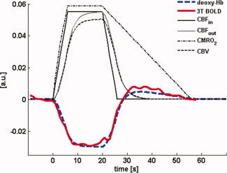
Time evolution of the parameters in the ‘arteriolar balloon’ model. CBFin and CMRO2 are the input parameters, where CBFin is modelled as a trapezoidal function and CMRO2 takes an assumed form that after stimulus offset ramps down linearly over the duration of the observed undershoot. The resulting arteriolar outflow CBFout (i.e. the inflow into the capillaries) depends on CBV, the volume of the arteriolar balloon. The experimentally measured response (T 2‐weighted BOLD at 3T, shown inverted) very closely follows the modelled deoxyhemoglobin response to a 20 s stimulus; this demonstrates the plausibility of arteriolar ballooning as explanation for the observed latency of the undershoot in the presence of sustained post‐stimulus elevation of CMRO2. Curves were arbitrarily rescaled for display. For details on model parameters see text. [Color figure can be viewed in the online issue, which is available at wileyonlinelibrary.com.]
For the set of typical model parameters, the response predicted by the ‘arteriolar balloon model’ agrees very well with the experimental data. The model calculations thus demonstrate the plausibility of a mechanism by which the BOLD undershoot is caused by sustained elevation in CMRO2, and its temporal characteristics are determined by a delayed compliance effect on the inflow side.
CONCLUSIONS
In this work, we have presented a straightforward way of investigating the BOLD undershoot with a purely T 2‐weighted fMRI sequence, and by taking advantage of the field‐strength dependence of contributions to the BOLD contrast. The attractiveness of the approach lies in the fact that clear insights can be gained without the need for more complicated techniques. We present strong evidence that the origin of the post‐stimulus BOLD undershoot is deoxyhaemoglobin accumulation in the small vessels following cessation of the neuronal activity; this is consistent with the notion of sustained post‐stimulus oxygen consumption. Our data reveal strongly point towards a sustained elevation in deoxyhaemoglobin level as the source of the post‐stimulus undershoot; blood flow and oxygen consumption are hence decoupled from each other. It appears from these data that neither parenchymal nor venous CBV changes alone can universally explain the undershoot. In addition we show that in the presence of a post‐stimulus elevation in CMRO2 the observed shape of the undershoot could be explained by delayed compliance of an arteriolar balloon as initially proposed by Behzadi and Liu [2005].
Supporting information
Additional Supporting Information may be found in the online version of this article.
Supporting Information Figure 1.
Supporting Information Figure 2.
Supporting Information Figure 3.
Supporting Information Materials.
Acknowledgements
The work presented in this paper was supported by STW (Dutch Technical Science Foundation) project NGT.6154. The authors would like to thank Siemens Medical Solutions in Erlangen, Germany for very kindly providing the two 32‐channel head coils, Markus Barth helping out with the data acquisition and for useful discussions throughout the project, and Oliver Langner for preparing the stimulus material.
REFERENCES
- Ances BM, Buerk DG, Greenberg JH, Detre JA ( 2001): Temporal dynamics of the partial pressure of brain tissue oxygen during functional forepaw stimulation in rats. Neurosci Lett 306( 1–2): 106–110. [DOI] [PubMed] [Google Scholar]
- Attwell D, Laughlin SB ( 2001): An energy budget for signaling in the grey matter of the brain. J Cereb Blood Flow Metab 21( 10): 1133–1145. [DOI] [PubMed] [Google Scholar]
- Behzadi Y, Liu TT ( 2005): An arteriolar compliance model of the cerebral blood flow response to neural stimulus. Neuroimage 25( 4): 1100–1111. [DOI] [PubMed] [Google Scholar]
- Berwick J, Johnston D, Jones M, Martindale J, Redgrave P, McLoughlin N, Schiessl I, Mayhew JE ( 2005): Neurovascular coupling investigated with two‐dimensional optical imaging spectroscopy in rat whisker barrel cortex. Eur J Neurosci 22( 7): 1655–1666. [DOI] [PubMed] [Google Scholar]
- Brockhaus J, Ballanyi K, Smith JC, Richter DW ( 1993): Microenvironment of respiratory neurons in the in vitro brainstem‐spinal cord of neonatal rats. J Physiol 462: 421–445. [DOI] [PMC free article] [PubMed] [Google Scholar]
- Buxton RB, Wong EC, Frank LR ( 1998): Dynamics of blood flow and oxygenation changes during brain activation: The balloon model. Magn Reson Med 39( 6): 855–864. [DOI] [PubMed] [Google Scholar]
- Chen JJ, Pike GB ( 2009): Origins of the BOLD post‐stimulus undershoot. Neuroimage 46( 3): 559–568. [DOI] [PubMed] [Google Scholar]
- Constable RT, Kennan RP, Puce A, McCarthy G, Gore JC ( 1994): Functional NMR imaging using fast spin echo at 1.5 T. Magn Reson Med 31( 6): 686–690. [DOI] [PubMed] [Google Scholar]
- Devor A, Dunn AK, Andermann ML, Ulbert I, Boas DA, Dale AM ( 2003): Coupling of total hemoglobin concentration, oxygenation, and neural activity in rat somatosensory cortex. Neuron 39( 2): 353–359. [DOI] [PubMed] [Google Scholar]
- Devor A, Hillman EM, Tian P, Waeber C, Teng IC, Ruvinskaya L, Shalinsky MH, Zhu H, Haslinger RH, Narayanan SN, Ulbert I, Dunn AK, Lo EH, Rosen BR, Dale AM, Kleinfeld D, Boas DA ( 2008): Stimulus‐induced changes in blood flow and 2‐deoxyglucose uptake dissociate in ipsilateral somatosensory cortex. J Neurosci 28( 53): 14347–14357. [DOI] [PMC free article] [PubMed] [Google Scholar]
- Devor A, Tian P, Nishimura N, Teng IC, Hillman EM, Narayanan SN, Ulbert I, Boas DA, Kleinfeld D, Dale AM ( 2007): Suppressed neuronal activity and concurrent arteriolar vasoconstriction may explain negative blood oxygenation level‐dependent signal. J Neurosci 27( 16): 4452–4459. [DOI] [PMC free article] [PubMed] [Google Scholar]
- Donahue MJ, Stevens RD, de Boorder M, Pekar JJ, Hendrikse J, van Zijl PC ( 2009): Hemodynamic changes after visual stimulation and breath holding provide evidence for an uncoupling of cerebral blood flow and volume from oxygen metabolism. J Cereb Blood Flow Metab 29( 1): 176–185. [DOI] [PMC free article] [PubMed] [Google Scholar]
- Duong TQ, Kim SG ( 2000): In vivo MR measurements of regional arterial and venous blood volume fractions in intact rat brain. Magn Reson Med 43( 3): 393–402. [DOI] [PubMed] [Google Scholar]
- Duong TQ, Yacoub E, Adriany G, Hu X, Ugurbil K, Kim SG ( 2003): Microvascular BOLD contribution at 4 and 7 T in the human brain: Gradient‐echo and spin‐echo fMRI with suppression of blood effects. Magn Reson Med 49( 6): 1019–1027. [DOI] [PubMed] [Google Scholar]
- Feng CM, Liu HL, Fox PT, Gao JH ( 2001): Comparison of the experimental BOLD signal change in event‐related fMRI with the balloon model. NMR Biomed 14( 7–8): 397–401. [DOI] [PubMed] [Google Scholar]
- Frahm J, Baudewig J, Kallenberg K, Kastrup A, Merboldt KD, Dechent P ( 2008): The post‐stimulation undershoot in BOLD fMRI of human brain is not caused by elevated cerebral blood volume. Neuroimage 40( 2): 473–481. [DOI] [PubMed] [Google Scholar]
- Frahm J, Kruger G, Merboldt KD, Kleinschmidt A ( 1996): Dynamic uncoupling and recoupling of perfusion and oxidative metabolism during focal brain activation in man. Magn Reson Med 35( 2): 143–148. [DOI] [PubMed] [Google Scholar]
- Friston KJ, Mechelli A, Turner R, Price CJ ( 2000): Nonlinear responses in fMRI: The Balloon model, Volterra kernels, and other hemodynamics. Neuroimage 12( 4): 466–477. [DOI] [PubMed] [Google Scholar]
- Gu H, Stein EA, Yang Y ( 2005): Nonlinear responses of cerebral blood volume, blood flow and blood oxygenation signals during visual stimulation. Magn Reson Imaging 23( 9): 921–928. [DOI] [PubMed] [Google Scholar]
- Harel N, Lee SP, Nagaoka T, Kim DS, Kim SG ( 2002): Origin of negative blood oxygenation level‐dependent fMRI signals. J Cereb Blood Flow Metab 22( 8): 908–917. [DOI] [PubMed] [Google Scholar]
- Hillman EM, Devor A, Bouchard MB, Dunn AK, Krauss GW, Skoch J, Bacskai BJ, Dale AM, Boas DA ( 2007): Depth‐resolved optical imaging and microscopy of vascular compartment dynamics during somatosensory stimulation. Neuroimage 35( 1): 89–104. [DOI] [PMC free article] [PubMed] [Google Scholar]
- Hoge RD, Atkinson J, Gill B, Crelier GR, Marrett S, Pike GB ( 1999): Stimulus‐dependent BOLD and perfusion dynamics in human V1. Neuroimage 9( 6 Pt 1): 573–585. [DOI] [PubMed] [Google Scholar]
- Jasdzewski G, Strangman G, Wagner J, Kwong KK, Poldrack RA, Boas DA ( 2003): Differences in the hemodynamic response to event‐related motor and visual paradigms as measured by near‐infrared spectroscopy. Neuroimage 20( 1): 479–488. [DOI] [PubMed] [Google Scholar]
- Jin T, Kim SG ( 2008a): Cortical layer‐dependent dynamic blood oxygenation, cerebral blood flow and cerebral blood volume responses during visual stimulation. Neuroimage 43( 1): 1–9. [DOI] [PMC free article] [PubMed] [Google Scholar]
- Jin T, Kim SG ( 2008b): Improved cortical‐layer specificity of vascular space occupancy fMRI with slab inversion relative to spin‐echo BOLD at 9.4 T. Neuroimage 40( 1): 59–67. [DOI] [PMC free article] [PubMed] [Google Scholar]
- Jochimsen TH, Norris DG, Mildner T, Moller HE ( 2004): Quantifying the intra‐ and extravascular contributions to spin‐echo fMRI at 3 T. Magn Reson Med 52( 4): 724–732. [DOI] [PubMed] [Google Scholar]
- Jones RA ( 1999): Origin of the signal undershoot in BOLD studies of the visual cortex. NMR Biomed 12( 5): 299–308. [DOI] [PubMed] [Google Scholar]
- Kennan RP, Zhong J, Gore JC ( 1994): Intravascular susceptibility contrast mechanisms in tissues. Magn Reson Med 31( 1): 9–21. [DOI] [PubMed] [Google Scholar]
- Kim T, Hendrich KS, Masamoto K, Kim SG ( 2007): Arterial versus total blood volume changes during neural activity‐induced cerebral blood flow change: implication for BOLD fMRI. J Cereb Blood Flow Metab 27( 6): 1235–1247. [DOI] [PubMed] [Google Scholar]
- Kong Y, Zheng Y, Johnston D, Martindale J, Jones M, Billings S, Mayhew J ( 2004): A model of the dynamic relationship between blood flow and volume changes during brain activation. J Cereb Blood Flow Metab 24( 12): 1382–1392. [DOI] [PubMed] [Google Scholar]
- Kwong KK, Belliveau JW, Chesler DA, Goldberg IE, Weisskoff RM, Poncelet BP, Kennedy DN, Hoppel BE, Cohen MS, Turner R, et al. ( 1992): Dynamic magnetic resonance imaging of human brain activity during primary sensory stimulation. Proc Natl Acad Sci USA 89( 12): 5675–5679. [DOI] [PMC free article] [PubMed] [Google Scholar]
- Lee SP, Duong TQ, Yang G, Iadecola C, Kim SG ( 2001): Relative changes of cerebral arterial and venous blood volumes during increased cerebral blood flow: Implications for BOLD fMRI. Magn Reson Med 45( 5): 791–800. [DOI] [PubMed] [Google Scholar]
- Lu H, Donahue MJ, van Zijl PC ( 2006): Detrimental effects of BOLD signal in arterial spin labeling fMRI at high field strength. Magn Reson Med 56( 3): 546–552. [DOI] [PubMed] [Google Scholar]
- Lu H, Golay X, Pekar JJ, van Zijl PCM ( 2003): Functional magnetic resonance Imaging based on changes in vascular space occupancy. Magn Reson Med 50( 2): 263–274. [DOI] [PubMed] [Google Scholar]
- Lu HZ, Golay X, Pekar JJ, van Zijl PCM ( 2004): Sustained poststimulus elevation in cerebral oxygen utilization after vascular recovery. J Cereb Blood Flow Metab 24( 7): 764–770. [DOI] [PubMed] [Google Scholar]
- Mandeville JB, Marota JJ, Ayata C, Zaharchuk G, Moskowitz MA, Rosen BR, Weisskoff RM ( 1999): Evidence of a cerebrovascular postarteriole windkessel with delayed compliance. J Cereb Blood Flow Metab 19( 6): 679–689. [DOI] [PubMed] [Google Scholar]
- Mildner T, Norris DG, Schwarzbauer C, Wiggins CJ ( 2001): A qualitative test of the balloon model for BOLD‐based MR signal changes at 3T. Magn Reson Med 46( 5): 891–899. [DOI] [PubMed] [Google Scholar]
- Nagaoka T, Zhao F, Wang P, Harel N, Kennan RP, Ogawa S, Kim SG ( 2006): Increases in oxygen consumption without cerebral blood volume change during visual stimulation under hypotension condition. J Cereb Blood Flow Metab 26( 8): 1043–1051. [DOI] [PubMed] [Google Scholar]
- Norris DG, Zysset S, Mildner T, Wiggins CJ ( 2002): An investigation of the value of spin‐echo‐based fMRI using a Stroop color‐word matching task and EPI at 3 T. Neuroimage 15( 3): 719–726. [DOI] [PubMed] [Google Scholar]
- Obata T, Liu TT, Miller KL, Luh WM, Wong EC, Frank LR, Buxton RB ( 2004): Discrepancies between BOLD and flow dynamics in primary and supplementary motor areas: Application of the balloon model to the interpretation of BOLD transients. Neuroimage 21( 1): 144–153. [DOI] [PubMed] [Google Scholar]
- Ogawa S, Menon RS, Tank DW, Kim SG, Merkle H, Ellermann JM, Ugurbil K ( 1993): Functional brain mapping by blood oxygenation level‐dependent contrast magnetic resonance imaging. A comparison of signal characteristics with a biophysical model. Biophys J 64( 3): 803–812. [DOI] [PMC free article] [PubMed] [Google Scholar]
- Parkes LM, Schwarzbach JV, Bouts AA, Deckers RH, Pullens P, Kerskens CM, Norris DG ( 2005): Quantifying the spatial resolution of the gradient echo and spin echo BOLD response at 3 Tesla. Magn Reson Med 54( 6): 1465–1472. [DOI] [PubMed] [Google Scholar]
- Poser BA, Norris DG ( 2007a): Fast spin echo sequences for BOLD functional MRI. Magn Reson Mater Phy 20( 1): 11–17. [DOI] [PMC free article] [PubMed] [Google Scholar]
- Poser BA, Norris DG ( 2007b): Measurement of activation‐related changes in cerebral blood volume: VASO with single‐shot HASTE acquisition. Magn Reson Mater Phy 20( 2): 63–7. [DOI] [PMC free article] [PubMed] [Google Scholar]
- Renvall V, Hari R ( 2009): Transients may occur in functional magnetic resonance imaging without physiological basis. Proc Natl Acad Sci USA 106( 48): 20510–20514. [DOI] [PMC free article] [PubMed] [Google Scholar]
- Sadaghiani S, Ugurbil K, Uludag K ( 2009): Neural activity‐induced modulation of BOLD poststimulus undershoot independent of the positive signal. Magn Reson Imag 27( 8): 1030–1038. [DOI] [PubMed] [Google Scholar]
- Schroeter ML, Kupka T, Mildner T, Uludag K, von Cramon DY ( 2006): Investigating the post‐stimulus undershoot of the BOLD signal—A simultaneous fMRI and fNIRS study. Neuroimage 30( 2): 349–358. [DOI] [PubMed] [Google Scholar]
- Shmuel A, Augath M, Oeltermann A, Logothetis NK ( 2006): Negative functional MRI response correlates with decreases in neuronal activity in monkey visual area V1. Nat Neurosci 9( 4): 569–577. [DOI] [PubMed] [Google Scholar]
- Turner R, Thomas D ( 2006): Cerebral Blood Volume: Measurement and Change. Proceedings 14th Scientific Meeting, International Society for Magnetic Resonance in Medicine, Seattle; p 2771.
- Tuunanen PI, Vidyasagar R, Kauppinen RA ( 2006): Effects of mild hypoxic hypoxia on poststimulus undershoot of blood‐oxygenation‐level‐dependent fMRI signal in the human visual cortex. Magn Reson Imaging 24( 8): 993–999. [DOI] [PubMed] [Google Scholar]
- Uludag K, Dubowitz DJ, Yoder EJ, Restom K, Liu TT, Buxton RB ( 2004): Coupling of cerebral blood flow and oxygen consumption during physiological activation and deactivation measured with fMRI. Neuroimage 23( 1): 148–155. [DOI] [PubMed] [Google Scholar]
- van Zijl PC, Eleff SM, Ulatowski JA, Oja JM, Ulug AM, Traystman RJ, Kauppinen RA ( 1998): Quantitative assessment of blood flow, blood volume and blood oxygenation effects in functional magnetic resonance imaging. Nat Med 4( 2): 159–167. [DOI] [PubMed] [Google Scholar]
- Villringer A, Them A, Lindauer U, Einhaupl K, Dirnagl U ( 1994): Capillary perfusion of the rat brain cortex. An in vivo confocal microscopy study. Circ Res 75( 1): 55–62. [DOI] [PubMed] [Google Scholar]
- Wu CW, Chuang KH, Wai YY, Wan YL, Chen JH, Liu HL ( 2008): Vascular space occupancy‐dependent functional MRI by tissue suppression. J Magn Reson Imaging 28( 1): 219–226. [DOI] [PubMed] [Google Scholar]
- Yacoub E, Ugurbil K, Harel N ( 2006): The spatial dependence of the poststimulus undershoot as revealed by high‐resolution BOLD‐ and CBV‐weighted fMRI. J Cereb Blood Flow Metab 26( 5): 634–644. [DOI] [PubMed] [Google Scholar]
- Zhao F, Jin T, Wang P, Kim SG ( 2007): Improved spatial localization of post‐stimulus BOLD undershoot relative to positive BOLD. Neuroimage 34( 3): 1084–1092. [DOI] [PMC free article] [PubMed] [Google Scholar]
Associated Data
This section collects any data citations, data availability statements, or supplementary materials included in this article.
Supplementary Materials
Additional Supporting Information may be found in the online version of this article.
Supporting Information Figure 1.
Supporting Information Figure 2.
Supporting Information Figure 3.
Supporting Information Materials.