Creating probabilistic maps of the face network in the adolescent brain: A multicentre functional MRI study

Abstract

Large‐scale magnetic resonance (MR) studies of the human brain offer unique opportunities for identifying genetic and environmental factors shaping the human brain. Here, we describe a dataset collected in the context of a multi‐centre study of the adolescent brain, namely the IMAGEN Study. We focus on one of the functional paradigms included in the project to probe the brain network underlying processing of ambiguous and angry faces. Using functional MR (fMRI) data collected in 1,110 adolescents, we constructed probabilistic maps of the neural network engaged consistently while viewing the ambiguous or angry faces; 21 brain regions responding to faces with high probability were identified. We were also able to address several methodological issues, including the minimal sample size yielding a stable location of a test region, namely the fusiform face area (FFA), as well as the effect of acquisition site (eight sites) and scanner (four manufacturers) on the location and magnitude of the fMRI response to faces in the FFA. Finally, we provided a comparison between male and female adolescents in terms of the effect sizes of sex differences in brain response to the ambiguous and angry faces in the 21 regions of interest. Overall, we found a stronger neural response to the ambiguous faces in several cortical regions, including the fusiform face area, in female (vs. male) adolescents, and a slightly stronger response to the angry faces in the amygdala of male (vs. female) adolescents. Hum Brain Mapp, 2012. © 2011 Wiley Periodicals, Inc.

INTRODUCTION

There is growing interest in explaining the role of environment, genes and their interplay in shaping the structure and function of the human brain. Given the variety of environmental factors and the challenges of genetics of complex traits, these questions are best addressed at a population level, hence the emergence of population neuroscience as a field situated at the intersection of cognitive neuroscience, genetics and epidemiology [Paus,2010]. In this context, magnetic resonance imaging (MRI), structural and functional, is the most common tool used to derive a large variety of quantitative brain phenotypes. In studies of brain development, structural MRI has been used on a large scale in three projects, namely in a cohort established in the Child Psychiatry Branch of the National Institutes of Mental Health [NIMH‐CHPB; Lenroot et al.,2007], NIH Pediatric MRI Database [NIH‐PD; Evans et al.,2006], and the Saguenay Youth Study [SYS: Pausova et al.,2007]. More recently, functional MRI has been incorporated in a multi‐centre study of the genetic and neurobiological bases of individual variability in impulsivity, reinforcer sensitivity and emotional reactivity in an adolescent population [IMAGEN; Schumann et al., 2010].

One of the unique opportunities offered by large‐scale MRI studies is the possibility to define the brain response to a certain stimulus at the population level. This can be achieved by constructing probabilistic maps that indicate the probability, from 0 to 100%, of “activating” a given 3D location (voxel) by the stimulus in a standardized atlas space. Such maps are similar to “ALE” (Activation Likelihood Estimate) maps [Turkeltaub et al.,2002], which are based on meta‐analyses of published functional imaging studies [e.g., Caspers et al.,2010; Fusar‐Poli et al.,2009]. In general, probabilistic maps are helpful in defining a priori regions‐of‐interest (ROI) characterized by a robust brain response to the stimulus in a given population. Such a reduction of fMRI data, from a voxel‐wise consideration of the entire brain to the ROI‐based focus on the most relevant brain regions, may be particularly useful in large‐scale genetic studies that often face Type I (false positive) error. Furthermore, probability maps can be utilized not only for defining ROIs but also as priors in the statistical analyses of the functional data. We will illustrate how the probability of “activation” can be used as weighting filter when calculating the peak and mean blood oxygenation‐level dependent (BOLD) response in a given ROI.

Here, we describe a novel approach for creating probabilistic maps of the neural network engaged consistently by the ambiguous or angry faces. These maps are constructed using fMRI data collected in the context of the IMAGEN study of the adolescent brain [Schumann et al., 2010]. IMAGEN is a genetic study focused on neural predictors of behavioral traits relevant for addiction. The “Face task” has been included in the fMRI battery to characterize the neural response to socially relevant stimuli, a feature of great importance especially in the context of adolescence when peer–peer interactions play a key role in shaping the adolescent behavior [Steinberg,2005; Steinberg and Silverberg,1986]. Extraction and processing of information from a face require the coordinated engagement of a number of brain regions. The three key components of the face network are the fusiform face area (FFA), regions along the superior temporal sulcus (STS), and the amygdala. Based upon lesion literature, these three regions likely contribute to different aspects of face processing [Adolphs et al.,2008; Akiyama et al.,2006; Tranel et al.,2009]. Furthermore, given the consistent albeit moderate advantage of girls over boys in face processing [McClure,2000], it is likely that the brain response to faces will vary in its magnitude as a function of the participant's sex. In previous studies, however, both the presence and directionality of such sex differences have been inconsistent, perhaps due to the variety of facial expressions investigated in the different studies [e.g., Aleman and Swart,2008; Ino et al.,2010; Rahko et al.,2010]. Here, we will take advantage of the large sample size and calculate effect sizes for the sex differences in the neural response to the ambiguous and angry faces across the key nodes of the “face network.”

While creating the probabilstic maps of the “face network.” we had the opportunity to explore some of the key methodological issues related to the multi‐centre nature of functional MRI studies. Previously, Zou et al. [2005] examined the impact of several sources of variability in multicentre studies, such as subject, study site, and scanner manufacturer, on the reproducibility of fMRI studies. They reported a significant effect of variability due to subject and scanner manufacturer on reproducibility measures such as sensitivity and specificity. Friedman et al. [2006,2008] initiated a series of experiments, referred to as Function Biomedical Informatics Research Network (fBIRN), to investigate the effect of variation due to scanner performance on the effect size of the functional response in multicentre fMRI studies. They reported significant effects of scanner on both factors. They also showed that an equalization of smoothness of fMRI data from different scanners reduces such effects. Similarly, Costafreda et al. [2007] investigated between‐scanner differences on reproducibility of fMRI studies using a similar scanner located at geographically different sites. Their results showed that the variability of the magnitude and extent of the functional response was driven more by intersubject differences than intersite variability. Here, we have been able to determine the minimal sample size necessary to identify a stable location of the FFA, and the effect of acquisition site and scanner on the location and magnitude of fMRI response to faces in this brain region.

MATERIALS AND METHODS

Participants

Participants involved in the IMAGEN Study include typically developing adolescents (13–15 years of age) and their families recruited at eight sites located in England (2 sites), France (1 site), Ireland (1 site), and Germany (4 sites). Exclusion criteria included events likely to affect normal brain development, such as premature birth, personal history of serious medical, neurological and/or psychiatric conditions, and low general intelligence (IQ <70); the list of all exclusion criteria can be found in Schumann et al. [2010] (Supporting Information Table II). The specific age‐range of the IMAGEN participants has been chosen to allow for the initial assessment and a subsequent follow‐up to occur in the mid‐to‐late adolescence when the pattern of substance use is most dynamic.

Table II.

MNI coordinates and probability values extracted from the probabilistic maps of the ambiguous faces vs. control and angry faces vs. control stimuli contrasts

No.	Label	Hemisphere	Lobe	Ambiguous face				Angry face
				MNI coordinate			Probability value (%)	MNI coordinate			Probability value (%)
				X	Y	Z		X	Y	Z
1	MVL‐FC	Left	Frontal	−42	27	−3	64	−42	27	−8	22
2	MVL‐FC	Right	Frontal	53	27	−3	100	53	27	4	71
3	MDL‐FC	Left	Frontal	−45	15	22	100	−42	15	24	68
4	MDL‐FC	Right	Frontal	46	20	20	100	44	20	22	96
5	PMC	Right	Frontal	51	5	46	100	48	3	48	86
6	Pre‐SMA	Right	Frontal	6	12	63	96	6	9	63	61
7	Rhinal Sulcus	Right	Temporal	42	−6	−44	64	40	−3	−44	50
8	Anterior STS	Right	Temporal	55	9	−24	100	54	6	−21	78
9	Posterior STS	Left	Temporal	−54	−51	9	100	−54	−48	6	82
10	Posterior STS	Right	Temporal	56	−42	7	100	54	−41	7	100
11	FFA	Left	Occipital	−40	−49	−22	100	−41	−48	−23	93
12	FFA	Right	Occipital	42	−49	−23	100	42	−48	−24	100
13	LOC	Left	Occipital	−45	−84	−12	86	−42	−84	−14	71
14	LOC	Right	Occipital	47	−78	−8	100	45	−79	−10	96
15	V2‐V3	Left	Occipital	−24	−99	0	78	−15	−102	−6	71
16	V2‐V3	Right	Occipital	24	−99	0	78	18	−102	0	57
17	Cerebellum	Left		−18	−78	−36	100	−17	−79	−36	75
18	Cerebellum	Right		18	−78	−39	57	18	−78	−37	11
19	Putamen	Right		21	6	6	57	21	6	0	32
20	Amygdala	Left		−18	−9	−15	96	−18	−9	−15	93
21	Amygdala	Right		22	−8	−14	100	20	−9	−17	100

The coordinates were determined as the centroids of regions with highest probability in the ambiguous vs. control map. Subsequently, the nearest coordinates with the highest probability value were found in the angry vs. control map. MVL‐FC, mid ventrolateral frontal cortex; MDL‐FC, mid dorsolateral frontal cortex; PMC, premotor cortex; preSMA, presupplementary motor area; STS, superior temporal sulcus; FFA, fusiform face area; and LOC, lateral occipital cortex.

Given the target age (14 years) of adolescents recruited in the IMAGEN project, we have excluded 26 participants outside of the age range between 13.5 and 15.5 years‐old. Across the eight acquisition sites, the mean age varied between 14.3 and 14.6 years, with standard deviations varying between 0.3 and 0.5 years. There were no significant differences in age between girls and boys at any site. As shown in Table I, however, the number of girls and boys was very different across the eight sites. To avoid any biases due to sex (and sex by site interaction), all analyses reported in this article include groups of adolescents with an equal number of girls and boys from the same acquisition site.

Table I.

Number of scanned adolescents/number of adolescents who passed quality control of the preprocessing pipeline across the eight sites

Site/Sex	Boys	Girls
Site1	55/54	130/119
Site2	95/94	64/63
Site3	83/72	66/62
Site4	59/42	77/60
Site5	73/70	101/97
Site6	74/66	86/72
Site7	75/69	74/67
Site8	58/51	53/52
Total	572/518	651/592

Adolescents and their families are recruited primarily through local high schools based on two key criteria: (a) ethnic homogeneity; and (b) sample diversity in terms of socioeconomic status, academic achievement, and behavioral/emotional functioning. Local ethics boards approved the study protocol; the parents and adolescents provided written informed consent and assent, respectively.

For the current report, structural and functional MR data were available in 1,223 adolescents; MR data obtained in 1,110 adolescents were retained after excluding participants outside the eligible age and/or failed quality‐control of the preprocessed images (see below for details). Table I indicates the distribution of the adolescents across the eight acquisition sites.

Magnetic Resonance Imaging: Acquisition

Structural and functional MR imaging is performed on 3 Tesla scanners from four manufacturers (Siemens: 4 sites, Philips: 2 sites, General Electric: 1 site, and Bruker: 1 site). The details of the entire MR protocol are described elsewhere [Schumann et al., 2010). This report utilizes T1‐weighted images and functional MR images collected during the Face paradigm. High‐resolution T1‐weighted anatomical images were acquired using 3D Magnetization Prepared Rapid Acquisition Gradient Echo (MPRAGE) sequence (TR = 2,300 msec; TE = 2.8 msec; flip angle = 9°; resolution: 1 × 1 × 1 mm³). Functional T2*‐weighted images were acquired using Gradient‐Echo Echo‐Planar‐Imaging (GE‐EPI) sequences (field of view: 22 cm; voxel size: 3.3 × 3.3 mm²; slice thickness of 2.4 mm; TE = 30 ms and TR = 2,200 ms; flip angle: 75°). The same set of parameters was used across all scanners with the following two exceptions: (1) parallel imaging was not used for the Bruker scanner during fMRI image acquisition; and (2) the order of in‐ and through‐plane phase encoding directions was swapped for the Philips scanner to match other scanners (i.e., first through‐plane and then in‐plane slice encoding).

Functional Paradigm: The Face task

The Face task involves passive viewing of videoclips that display ambiguous (emotionally “neutral”) or angry face expressions or control (nonbiological motion) stimuli [Grosbras and Paus,2006]. Each trial consists of short (2 to 5 s) black‐and‐white videoclips depicting either a face in movement or the control stimulus (see Fig. 1). The control stimuli consist of black‐and‐white concentric circles of various contrasts, expanding and contracting at various speeds, roughly matching the contrast and motion characteristics of the face clips. These control stimuli were adapted from a study of Beauchamp et al. [2003]. Luminance and contrast were equalized and a gamma correction was applied. The stimuli are presented through goggles (Nordic Neurolabs, Bergen, Norway) in the scanner and subtend a visual angle of 10° × 7°. The videoclips are arranged into 18‐s blocks; each block includes seven to eight videoclips. Five blocks of each biological‐motion condition (ambiguous, and angry faces), and nine blocks of the control condition (circles) are intermixed and presented to the participants using the Java‐based stimulus‐delivery software. To ensure that the stimuli are synchronized to the MR image acquisition, a signal sent from the scanner at the beginning of each image acquisition is converted into a TTL pulse transmitted to the stimulation computer through a USB port. The stimuli delivery software reads every sixth TTL pulse as a signal to start a new block. The entire fMRI run lasts six min.

Figure 1.

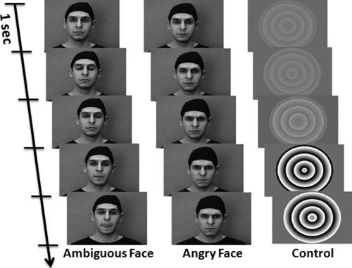
Stimuli presentation: Snapshots were taken at the beginning (initial one second) of representative clips of each condition. The video clips were displayed at 30 frames/s. Two consecutive images on the figure are separated by five frames.

Functional MR Images: Preprocessing

During scanning of each participant, a total of 160 EPI volumes were acquired in a single six‐min fMRI run. T1‐weighted and functional EPI data were preprocessed and analyzed at the single‐subject and group‐level using SPM8 software package (Statistical Parametric Mapping: Wellcome Department of Cognitive Neurology, London, UK).

EPI images were motion‐corrected with respect to the first volume using the realignment tool of SPM, namely with a least squares approach and a six‐parameter rigid‐body spatial transformation with fourth degree B‐Spline interpolation. A mean functional image and six realignment parameters (three translations and three rotations) per EPI volume were generated for each participant.

Subsequently, the EPI images and the high‐resolution T1‐weighted images of each participant were aligned together. For this purpose, skull‐stripped structural images were rigidly (six‐parameter transformation) registered to the mean EPI image using the Mutual Information co‐registration tool of SPM software. Skull stripping was done using the Brain Extraction Tool (BET) of the FSL software package (Oxford Centre for Functional MRI, Oxford University, UK).

Next, to render the data normally distributed and, as such, appropriate for parametric tests, the motion‐corrected EPI data were spatially smoothed using an isotropic Gaussian kernel of 6 mm FWHM [i.e., twice the voxel size: Worsley and Friston,1995].

Quality Control of Preprocessing Pipeline

The quality control (QC) of functional MR images focused on the artifacts due to motion during scanning. Using realignment parameters from the motion‐correction step in preprocessing pipeline, EPI volumes with parameter values exceeding 2 mm in translation or 2° in rotation errors (in any direction) were excluded: Participants with more than 20 flagged volumes were excluded from the pool altogether. Furthermore, visual QC carried out by three independent raters was used to identify errors due to rigid (EPI‐to‐T1W) and non‐rigid (T1W‐to‐ICBM152) registrations.

Functional Analysis

Smoothed EPI volumes from each participant were entered into the individual (fixed‐effects) general linear model (GLM). The hemodynamic response function was selected as the basis function. The six realignment parameters from motion‐correction were also included as regressors of no interest in the model to account for the effect of the residual head movements.

Two contrasts were considered in this study: (1) ambiguous faces vs. control stimuli; and (2) angry faces vs. control stimuli. The two sets of contrast images were generated per participant to be entered into a (second‐level) group analysis, treating the participant factor as a random effect. For this purpose, the contrast images were transformed to the ICBM152 template space [Mazziotta et al.,2001] using the deformation parameters from the nonlinear registration of the corresponding structural data (co‐registered with the mean EPI) to the ICBM152 template. The nonlinear registration was achieved using the Unified Segmentation tool in SPM package. Note that the correction of intensity inhomogeneity is embedded within the unified segmentation tool of SPM.

Functional Probabilistic Maps

We used two different strategies to generate probabilistic maps of the brain response to the ambiguous and angry faces. The first strategy (Fig. 2, left) combines an equal number of male and female adolescents “at entry,” namely at the point of calculating a given contrast (e.g., ambiguous vs. control); the resulting t‐statistics images are thresholded, binarized, and averaged. The second strategy (Fig. 2, right) differs from the first one in that a given contrast is calculated for each sex separately; the resulting sex‐specific t‐images are thresholded, binarized, and only then combined (as a union) across the two sexes. The latter approach decreases a possible exclusion of voxels “activated” by one sex only and, as such, it is well suited for the assessment of sex differences in the brain response to faces. We will now describe these two approaches in more detail.

Figure 2.

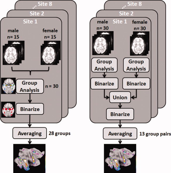
Flowchart illustration of the procedure for creating two types of functional probabilistic maps using functional data from eight acquisition sites: Left: sex combined at entry; and Right: sex combined after sex‐specific analyses.

Functional Probabilistic Maps: Sex Combined at Entry

As illustrated in Figure 2 (left), the functional probability maps for a desired contrast (ambiguous face vs. control; angry face vs. control) were constructed in the following way. Functional data from each acquisition site were grouped in as many independent sets as possible using a fixed sample‐size of 30 participants (see below for rationale) and considering equal number of boys (n = 15) and girls (n = 15) in each set; note that boys and girls from different acquisition sites are not “mixed” within a given set. Image data from each group were entered into second‐level analyses for generating the statistical parametric maps (t‐maps). The generated t‐maps were thresholded at P < 0.001 (uncorrected), binarized and averaged to construct a probabilistic map for a given fMRI contrast.

Functional Probabilistic Maps: Sex Combined After Sex‐Specific Analyses

As illustrated in Figure 2 (right), functional data from each acquisition site were grouped in as many independent sets as possible using a fixed sample‐size of 30 girls and 30 boys from each acquisition site. Image data from each sex‐specific group were entered into second‐level analyses for generating the statistical parametric maps (t‐maps). The generated t‐maps were thresholded at P < 0.001 (uncorrected) and binarized. Next, we created a union of as many “pairs” of the binarized maps obtained in girls and boys from the same acquisition site; the pairing was random. Finally, the combined “girl–boy” binarized maps were binarized and averaged to construct a probabilistic map for a given fMRI contrast.

High‐Probability Regions of Interest

To define brain regions (voxels) engaged by the ambiguous and angry faces with “high” probability in this adolescent sample, the generated probabilistic maps were thresholded at 50% and binarized (assigning value 1 to any voxel with probability value greater than or equal to 0.5). The resulting binary images were then divided into nonintersecting regions using a semiautomatic approach; an automatic region‐growing segmentation initialized with manually selected seed‐voxels was applied to each map. The resulting regions were manually corrected for any errors. Seed voxels were provided by an expert neuroanatomist. The X, Y, and Z coordinates of the center‐of‐mass of the extracted regions are reported for each ROI. Overall, 21 ROIs were identified in both hemispheres and across both probabilistic maps (ambiguous and angry). This is the case irrespective of the strategy used for creating the probabilistic maps, as described above. These ROIs represent brain regions engaged, with high probability, during the processing of ambiguous and angry faces in the sample of 1,110 adolescents; Table II lists these ROIs defined with the probabilistic maps created with the first strategy (i.e., sex combined at entry).

To obtain ROIs with the full range of probabilistic values, the extracted ROIs were further dilated using the original probability maps to include the rest of the voxels with probability values greater than 1% and less than 50% belonging to the same ROI that were initially excluded due to thresholding the maps at 50%. The stopping threshold for dilation was manually selected if two or more adjacent regions meet at voxels with arbitrary probability values. The resulting ROIs were finally validated by an expert neuroanatomist.

ROI‐based Measures of BOLD response

To quantify the BOLD response in each ROI, we first calculated the percent BOLD signal change (PBSC) by dividing the estimates of the parameters from the GLM (at fixed‐effects level), referred to as βs, by the mean of the baseline level (the intercept in the GLM), and multiplied these by 100. For each participant, we used the PBSC image and calculated the following three measures of fMRI response:

• 1Peak PBSC: Maximum value at any voxel within the selected ROI;
• 2Mean PBSC: Mean of PBSC values across all voxels within the selected ROI; and
• 3Number of active voxels (normalized): Ratio of voxels within the selected ROI whose values exceeded significance threshold of t = 1.96 (P = 0.001, uncorrected). over the total number of voxels constituting this ROI.

Merging Data across Multiple Acquisition Sites

In multi‐center fMRI studies, a major challenge in merging data across several acquisition sites is to detect and minimize the structured variances in data due to differences across scanners and acquisition sites to measure the variance in factors of interest, such as the BOLD response to the paradigm of interest. To evaluate the effects of acquisition site and scanner manufacturer, one can measure the reproducibility of the fMRI BOLD response with respect to (1) the location of the “activated” region; and (2) the magnitude of the response for a particular ROI.

For this purpose, we selected the FFA in the right hemisphere as a test ROI. FFA is one of the cortical regions engaged most strongly by face stimuli [Caspers et al.,2010; Fusar‐Poli et al.,2009; Kanwisher and Yovel,2006]. For the location, we first determined peak coordinates for the right FFA using the following approach. Second‐level analyses on fixed‐size samples of randomly selected participants, with an equal number of girls and boys, were conducted separately for each acquisition site. The peak location within the right FFA was identified in the resulting t‐statistics maps for the ambiguous vs. Control contrast. To determine coordinates of a “reference” FFA, we calculated the median of the peak coordinates obtained across the eight sites for the largest sample size of 80 participants per acquisition site. The various measures of the BOLD response were extracted from a cubic ROI (5 × 5 × 5 voxels) centered at the location of the right reference FFA.

RESULTS

Quality Control of Preprocessing Pipeline

In total, 57 participants were excluded due to extreme motion artifact in EPI image data. Furthermore, using visual QC by three raters, 19 participants were excluded due to registration errors (EPI‐to‐T1W and T1W‐to‐ICBM152). The distribution of participants across eight sites after passing motion and registration QC is given in Table I. The final sample includes 1,110 adolescents (592 girls, 518 boys).

Functional Probabilistic Maps: Sex Combined at Entry

As explained above, to generate the probabilistic maps, we have randomly selected as many independent sets of 30 participants from a given acquisition site (15 boys and 15 girls) to be entered to the second‐level analysis. This sample size was selected because it is the smallest sample size that yielded stable location of the right FFA (see below). Overall, there exist 28 independent groupings of participants with the aforementioned criteria; one acquisition site contributed only two such “n = 30” samples (Site 4) while most sites contributed four “n = 30” samples (Sites 2,3,5,6, and 7). A total of 840 participants (28 samples of 30 participants each) contributed to this analysis. The resulting t‐maps for each contrast (28 in total) were thresholded (P < 0.001, uncorrected) and binarized. The binary images were then averaged to generate the probabilistic maps termed henceforth the PM28 maps. Figure 3 shows the axial cross‐sections of the probability maps of the ambiguous and angry contrasts between the face and control stimuli superimposed on the average image generated using warped structural images of the participants who contributed to these probability maps. Figure 4 displays these probability maps on the flattened cerebral cortex, as generated using the CARET software [Van Essen et al.,2001].

Figure 3.

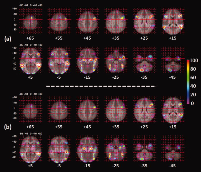
Axial cross‐sections of the probability maps of the (a) ambiguous and (b) angry contrasts between the face and control stimuli superimposed on the average image generated using 840 warped structural images of the participants who contributed to the probability maps. Numbers below the images correspond to the Z coordinates.

Figure 4.

Probability maps of the ambiguous (a) and angry (b) contrasts between the face and control stimuli displayed of the flatten cerebral cortex. The bottom image (c) provides reference to the location of the main cortical regions responding to the presentation of faces, including: FFA, fusiform face area; LOC, lateral occipital cortex; STS, superior temporal sulcus; preSMA, pre supplementary motor area; PMC, premotor cortex; MDL‐FC, mid dorsolateral frontal cortex; and MVL‐FC, mid ventrolateral frontal cortex. Left and right hemispheres are displayed on the left and right, respectively.

Measuring BOLD Response Using the Proposed Probabilistic ROIs

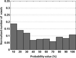
Peak PBSC, mean PBSC, and number of active voxels were calculated in two regions‐of‐interest well‐known as being engaged during the facial emotion processing, namely the right FFA and the right amygdala. These two ROIs were extracted from the PM28 probability map created for the ambiguous face contrast. Figures 5 and 6 show the distribution of the number of voxels (normalized) with respect to the probability value; as can be observed from both figures, both distributions are fairly close to uniform. The three BOLD measures were obtained in the following four ways: (a) all voxels with the entire range of probability values (i.e., 1 to 100%); (b) high probability voxels (i.e., 51 to 100%); (c) low probability voxels (i.e., 1 to 50%); and (d) including all nonzero voxels and weighting the BOLD response values at each given voxel by the corresponding probability value. The number of active voxels was not calculated for this type of ROI‐based analysis.

Figure 5.

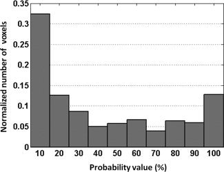
Distribution of the number of voxels (normalized between 0 and 1) with respect to the probability values of the right FFA.

Figure 6.

Distribution of the number of voxels (normalized between 0 and 1) with respect to the probability values of the right amygdala.

First, we used a one‐way ANOVA to compare the nonweighted (a) and weighted (d) values. In the right FFA, significant differences were observed for both the mean PBSC [F(1,2218) = 122.03, η² = 0.000*] and peak PBSC [F(1,2218) = 63.5, η² = 0.000*]. Similarly, in the right amygdala, differences were significant for both mean PBSC [F(1,2218) = 100.1, η² = 0.000*] and peak PBSC [F(1,2218) = 86.9, η² = 0.000*] Second, we used a one‐way ANOVA to compare the “high” (b) and “low” (c) probability voxels. Significant differences were observed for both the mean PBSC [F(1,2218) = 424.7, η² = 0.000*] and peak PBSC [F(1,2218) = 11.6, η² = 0.001] in the right FFA region. In the right amygdala, only the differences in the mean PBSC was significant [F(1,2218) = 310.5, η² = 0.000*].

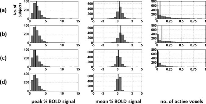
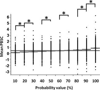
Figures 7 and 8 show the distributions of the Peak PBSC, mean PBSC and number of active voxels (normalized between 0 and 1) for all aforementioned cases of (a) to (d), within regions of the right FFA and right amygdala, respectively. As can be seen in Figures 7 and 8, the distributions of the Peak PBSC are very similar across the four comparisons while, as expected, those of the Mean PBSC and the number of active voxels are shifted to the left (lower values) for the low‐probability comparisons. The similarity of the distributions of the Peak BOLD between the low and high‐probability comparisons is somewhat surprising. We have therefore plotted both the frequency of the location (Figs. 9 and 10, top) and the value (Figs. 9 and 10, bottom) of the peak voxel as a function of its probability. As expected, the peak voxel is most often found in the high‐probability part of the ROI (35% of all peaks in the right FFA region and 30% of all the peaks in the right amygdala are found in voxels with probability higher than 90%). But as suggested by the similarity of the Peak PBSC distributions shown in Figures 7 and 8, the actual value of the Peak PBSC is independent of the probability of a given voxel being “active” at a population level. Figures 11 and 12 show the distribution of the mean PBSC with respect to the probability values within the right FFA and the right amygdala, respectively. Multivariate ANOVA test revealed a significant main effect of the threshold value [right FFA: F(9,11090) = 187.2, η² = 0.000*; right amygdala: F(9,11090) = 150.8, η² = 0.000*]. Further post hoc analyses (Sidak‐corrected for multiple comparisons, α = 0.05) revealed significant differences between almost every neighboring threshold values for both regions: 100% > 90% > 80% and 70% > 60% and 50% > 40% and 30% > 20% > 10%.

Figure 7.

Distribution of the peak BOLD response (first column), mean BOLD response (second column) and the number of active voxels (third column) in a region‐of‐interest around the right FFA, which was extracted from the probability map for the ambiguous face vs. control stimulus contrast. The four rows display the three measures obtained, with the aid of the probabilistic map, in the following four ways: (a) all voxels with all range of probability values (i.e., 1 to 100%); (b) high probability voxels (i.e., 51 to 100%); (c) low probability voxels (i.e., 1 to 50%); and (d) similar to (a) except that voxel measure is weighted by the corresponding probability value at each voxel. The median of each distribution is shown with a solid black line in each plot.

Figure 8.

Distribution of the peak BOLD response (first column), mean BOLD response (second column) and the number of active voxels (third column) in a region‐of‐interest around the right amygdala, which was extracted from the probability map for the ambiguous face vs. control stimulus contrast. The four rows display the three measures obtained, with the aid of the probabilistic map, in the following four ways: (a) all voxels with all range of probability values (i.e., 1 to 100%); (b) high probability voxels (i.e., 51 to 100%); (c) low probability voxels (i.e., 1 to 50%); and (d) similar to (a) except that voxel measure is weighted by the corresponding probability value at each voxel. The median of each distribution is shown with a solid black line in each plot.

Figure 9.

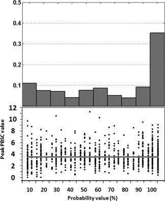
Frequency of the location (top) and the value (bottom) of the peak voxel in the right fusiform face area, which was extracted from the probability map for the ambiguous face vs. control stimulus contrast, as a function of its probability. The gray line presents the mean of the peak PBSC within the population.

Figure 10.

Frequency of the location (top) and the value (bottom) of the peak voxel in the right amygdala, which was extracted from the probability map for the ambiguous face vs. control stimulus contrast, as a function of its probability. The gray line presents the mean of the peak PBSC within the population.

Figure 11.

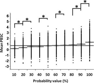
Distribution of the mean PBSC with respect to the threshold value extracted from the probability map for the ambiguous face vs. control stimulus contrast for the region of right FFA. (*) indicates a significant difference in post hoc comparisons. The gray line presents the group mean PBSC.

Figure 12.

Distribution of the mean PBSC with respect to the threshold value extracted from the probability map for the ambiguous face vs. control stimulus contrast for the region of right amygdala. (*) indicates a significant difference in post hoc comparisons. The gray line presents the group mean PBSC.

Sex Differences in the BOLD Response

Supporting Information Figures S1 and S2 provide sex‐specific probabilistic maps for the two contrasts; each map was created by averaging 13 sex‐specific binarized maps obtained by thresholding t‐images calculated in groups of 30 boys and 30 girls per acquisition site. Note the differences in the extent of the low‐probability regions in the case of ambiguous faces. For this reason, sex differences will be evaluated using the probabilistic maps created using the second strategy, namely the union of binarized maps calculated separately for boys and girls (see above). Overall, there exist 13 independent “pairs” of the boy and girl groups across the eight acquisition sites; three acquisition sites contributed only one such pair of “n = 30” samples per sex (Sites 1, 4, and 8) while the remaining sites contributed two “girls–boys” pairs. A total of 780 participants (26 samples of 30 participants each: 13 “girls” and 13 “boys” samples) contributed to this analysis. The resulting sex‐specific t‐maps for each contrast were thresholded (P < 0.001, uncorrected) and binarized. A union of the binary images for a given site‐specific “girls–boys” pair was generated and binarized. A total of 13 such binarized maps were then averaged to generate the probabilistic maps termed henceforth the PM13 maps.

The resulting probability maps were segmented to 21 ROIs using the same approach as described for the PM28 maps. For each ROI, we estimated an effect size of the sex difference using Cohen's d calculated for a given BOLD‐response measure. Cohen's d is defined as the difference between sex‐specific means of the BOLD response measures (in this case, the number of active voxels) divided by the pooled standard deviation of the sample population:

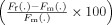
where and , and s are the mean, and standard deviation of the BOLD response measure and n refers to the number of females (f) and males (m) in each group. Figure 13 compares the Cohen's d measure of the number of active voxels for the ambiguous and angry face contrasts among the 21 ROIs in the left (top) and right (bottom) hemispheres. Positive and negative values represent higher number of active voxels for girls than boys, respectively. Supporting Information Tables S1 and S2 provide the mean and standard deviation of the number of active voxels and the weighted mean BOLD response for each sex and contrast. Both tables also include the percentage difference between girls and boys of the corresponding measures (F(.): weighted mean PBSC or normalized number of active voxels) and the Cohen's d. The p‐values resulting from ANOVA analyses (comparing each measure by sex per ROI) are also provided in the tables.

Figure 13.

Sex differences (Cohen's d; 592 girls, 518 boys) in the number of active voxels within 21 ROIs of the PM13. Positive and negative values represent higher number of active voxels for girls than boys and vice versa.

Effect of Sample Size, Acquisition Site, and Scanner

As described above, right FFA was selected as the test ROI for evaluating the effect of sample size, acquisition site, and scanner on the variability in the location and magnitude of the BOLD response to faces.

The group size for sampling the population in this study varies from 10 to 80 participants per acquisition site, with an equal number of boys and girls (refer to Table I). Despite the fact that studies with more participants will yield t‐maps with higher statistical power, the fMRI response fields should not vary significantly passing a certain sample size assuming that the effect of structural variability is negligible after registering all participants' images with the same template.

The minimum sample size that would be sufficient to preserve population characteristics in fMRI group analyses was determined using the following procedure. The individual (aligned) contrast images were combined, within a given acquisition site, using a range of sample sizes starting from 10 participants (5 boys and 5 girls) to the maximum of 80 participants (40 boys and 40 girls) with increments of 10 participants (5 boys and 5 girls). The location of the local maximum for the right FFA was determined in t‐maps of different sample sizes across all eight sites.

The effect of the sample size on the variability in the location of the FFA response was evaluated in two ways. First, we conducted three separate one‐way ANOVAs evaluating the effect of the sample size on X, Y, and Z coordinates of the local maximum in the right FFA region; no significant effect was observed [X: F(7,56) = 0.7, P = 0.7; Y: F(7,56) = 0.6, P = 0.8; Z: F(7,56) = 0.9, P = 0.5]. Second, we calculated the Euclidean distance between the location of the “reference” FFA (X = 42, Y = −48, Z = −23; see above) and the local maximum of the BOLD response in the right FFA (i.e., the voxel with the highest t value) obtained in each group (see Fig. 14). One‐way ANOVA of the Euclidean distances revealed a significant main effect of the sample size [F(3,636) = 3.158, η² = 0.024]. Post hoc comparisons (Sidak‐corrected for multiple comparisons to achieve α = 0.05) showed a significant difference between sample sizes of 10 and 20 participants versus those of 60 and 80 participants; there were no significant differences between groups with 30 through 80 participants. We took this as an evidence for determining the sample size n = 30 as the minimum size of a sample to yield reliable FFA location. We used this size for generating functional probabilistic maps described above.

Figure 14.

Euclidean distances for the different sample sizes (from 10 to 80 participants) calculated across the eight acquisition sites per sample. For each sample, we calculated the distance between the location of the right fusiform face area (FFA) obtained in this sample and its “reference” location. The “reference” location of the right FFA was defined as the median across the eight acquisition sites for the largest sample size of 80 participants (MNI coordinate: X = +42, Y = −48, Z = −23).

To evaluate the effect of the acquisition site on the location of the right FFA, we assessed the variability in X, Y, and Z coordinates of the local maximum within right FFA (extracted from t‐statistics maps) in a fixed sample size of n = 80 per acquisition site across the eight acquisition sites. The X coordinate was the same across all sites (X = +42), while the Y coordinate had two different values (Y = −48: six sites; and Y = −51: two sites). The most variation in the location was occurring along the z‐axis (Z = −18: one site; Z = −21: three sites; and Z = −24: four sites). Furthermore, the mean±std of the Euclidean distance between every pair of the extracted local maximum coordinates for the right FFA (from eight sites) was determined as 3.12 ± 2.04 (range: [0,6] mm). Also, there was no significant difference among four types of scanners (GE, Philips, Bruker and Siemens) in terms of the Euclidean distance error.

The effect of sample size on the magnitude of the BOLD signal was determined using an ANOVA test on the t‐statistics value at the peak activation foci in the right FFA region, which were identified by the group analyses with different sample sizes ranging from 10 to 80. As expected, there was a significant effect of the sample size [F(7,56) = 10.1, η² = 0.000*]. Further post hoc comparisons (Sidak‐corrected for multiple comparisons, α = 0.05) showed a significant difference between different sample sizes according to the following order (high to low): 80 > 70, 60 > 50, 40 > 30, 20, 10.

The effect of the acquisition site and scanner on the magnitude of the fMRI response was evaluated by conducting one‐way ANOVA on the three measures described above (Peak PBSC, Mean PBSC, and number of active voxels), which were calculated for a ROI defined around the reference FFA (X = 42,Y = −48, Z = −23; ROI size 5 × 5 × 5 voxels) for all individuals within the sample size 80 (40 boys and 40 girls) per site and across all eight sites. As seen in Figure 15, for the acquisition site (eight levels), ANOVA did not reveal any significant effects of the site on the peak and mean PBSC. There was a significant main effect of the acquisition site on the number of active voxels [F(7,632) = 2.1, η² = 0.044]. Further post hoc comparisons (Sidak‐corrected for multiple comparison, α = 0.05) showed a significant difference between two acquisition sites (Sites 4 and 5). For the scanner (four levels: GE, Philips, Siemens, and Bruker), ANOVA analysis revealed a significant main effect of the scanner on all three measures [peak PBSC: F(3,636) = 3.5, P = 0.02; mean PBSC: F(3,636) = 3.4, P = 0.02; number of active voxels: F(3,636) = 4.1, P = 0.007]. Post hoc comparisons showed a significant difference between Bruker (Site 4) and Philips for peak PBSC (Bruker < Philips), Bruker with Philips and Siemens for mean PBSC (Bruker < Philips, Bruker < Siemens), and Bruker with Siemens (Bruker < Siemens) for the number of active voxels.

Figure 15.

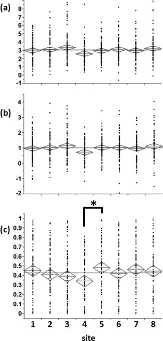
Functional MR response to ambiguous faces in the right fusiform face area. (a) Peak percent BOLD signal change; (b) mean percent BOLD signal change; and (c) normalized number of active voxels. Site indicates the eight acquisition sites (in no particular order). (*) indicates a significant difference in post hoc comparisons.

DISCUSSION

Using a large dataset of fMRI images acquired in typically developing adolescents in the context of a multi‐center study (IMAGEN), we were able to construct probabilistic maps of the neural network engaged consistently by the ambiguous or angry faces. These maps specify the likelihood of the neural response to the face stimulus at every voxel throughout the brain. We have also been able to address several methodological issues associated with multi‐site fMRI studies, to compare three different measures of the BOLD response and, finally, provide the initial description of sex differences in the brain response to faces. We will now address these topics in the text below.

Probabilistic maps presented here are based on fMRI data acquired in 840 adolescents (420 girls and 420 boys) who viewed the same videoclips of ambiguous and angry faces and were scanned using the same MR protocol implemented at eight acquisition sites. In this way, these maps differ from the ALE maps, which are based on a meta‐analysis of multiple fMRI studies acquired with different behavioral paradigms and different MR sequences at multiple geographical locations. Furthermore, typical ALE maps do not incorporate study‐specific differences in sample size and in the actual magnitude and extend of the fMRI response at a given location; all these parameters are considered when constructing probabilistic maps described here. Let us briefly compare our probabilistic maps with the ALE maps based on a meta‐analysis of 105 fMRI studies of face processing carried out by Fusar‐Poli et al. [2009]. This analysis included a total of 1,600 healthy participants; the number of participants per study varied between 5 and 40, with a mean of 15.2 participants. To compare the two datasets, we have transformed the X, Y, and Z coordinates reported in Fusar‐Poli et al. [2009] to the MNI coordinate frame using the transformation provided by Lancaster et al. [2007], and calculated Euclidean distance between the two sets of locations. For the ambiguous (or neutral) faces, the location of the right FFA is very similar (ROI 12 in Table II; Euclidean distance of 5.4 mm, with 93% probability of the Fusar‐Poli FFA in our probabilistic map). This is also true for the left amygdala (ROI 20 in Table II; Euclidean distance of 3.7 mm, with 86% probability of the Fusar‐Poli FFA in our probabilistic map). On the other hand, the location of a local maximum in the right mid‐dorsolateral frontal cortex differs across the two studies (ROI 04 in Table II; Euclidean distance of 11.6 mm, with 71% probability of the Fusar‐Poli FFA in our probabilistic map). For the angry faces, there is very little overlap between the ALE map and our map, with the exception of the left amygdala (ROI 21 in Table II), right posterior STS (ROI 10 in Table II) and the left cerebellum (ROI 17 in Table II). Thus, the two sets of probabilistic maps provide somewhat different picture of the “face network” both in qualitative (presence/absence of certain brain regions) and quantitative (exact location of a region) terms. This is not surprising given the large variety of stimuli and contrasts that are, by definition, included in any meta‐analysis and the uniformity of the face paradigm used in the IMAGEN study. One can argue that the two approaches are complementary in that the ALE‐based approach provides a survey of all brain regions “activated” by many kinds of face stimuli while the IMAGEN‐based probabilistic maps provide precise definitions of the face network engaged by a particular set of face stimuli. This precision may be of critical importance when one wishes to use such probabilistic maps to define regions of interest to analyze fMRI data obtained in independent studies.

The nature of the current dataset, namely its large size and multi‐site acquisition, allowed us to evaluate some of the basic sources of variability in the location and magnitude of the fMRI response to ambiguous and angry faces. As pointed out by others [Costafreda et al.,2007], one of the main sources of variability is the individual participant. Therefore, the first question we addressed was the consistency of the “peak” location as a function of number of participants. Comparing different sizes of samples available at all acquisition sites, from the smallest sample of 10 adolescents to the largest one of 80 adolescents per site, we have observed no significant variations in the location of the right FFA when comparing each of the three coordinates (X, Y, and Z) independently. We found, however, a subtle but significant effect of sample size on Euclidean distance: the smallest two samples (n = 10 and n = 20) were different from the larger ones. The between‐sample difference in the Euclidean distance at the sample‐size “boundary” (i.e., n = 20 vs. n = 30) was about 2 mm. Although rather small, such a shift in the “centre‐of‐gravity” of a region‐of‐interest can influence, for example, comparisons of two groups of participants vis‐à‐vis their fMRI response in what is presumed to be the same functional region. In this context, it should be noted that the majority of previous fMRI studies of face processing acquired data in about 15 participants per study (Range: 5 to 40 participants; 25th and 75th quartiles of 10 and 18 participants, respectively; Mean: 15.2; Standard Deviation: 7.1; Median = 13; from Fusar‐Poli et al. [2009]). Given that such studies are used in meta‐analyses carried out, for example, with ALE, one needs to be aware of the possible imprecision of ALE‐derived probabilistic maps.

One of the main reasons for multi‐centre neuroimaging studies is the relative efficiency with which one can collect large number of MRI datasets; in the IMAGEN project, the 1,110 adolescents have been scanned in less than two years. But as pointed out by others [e.g., Costafreda et al.,2007; Friedman et al.,2006,2008; Zou et al.,2005], acquiring data at several acquisition sites and using scanners made by different manufacturers can hamper pooling data across the sites. In the case of the FFA response to ambiguous (or emotionally “neutral”) faces, these undesirable sources of variance are rather small. First of all, we found very little variations in the location of the FFA across sites and scanners. Second, the only significant effect of acquisition site was observed for only one of the fMRI measures, namely the number of active voxels, and—based on post hoc statistical comparisons—this difference was significant only when comparing Site 4 vs. Site 5. It should be pointed out that, overall, the effect of site and scanner on the magnitude of the fMRI response in the right FFA explains only up to 2% of total variance. The effect of acquisition site is most likely related to the fact that data at Site 4 were acquired with a Bruker scanner; the effect of scanner is significant for most fMRI measures, with the post hoc statistical comparisons clearly indicating that the scanner effect is driven by differences between the Bruker scanner and both the Philips and Siemens scanners. This may be due to a slightly lower signal‐to‐noise ratio of the Bruker scanner, when compared with a Siemens scanner. Such a scanner effect is not surprising; it has been identified in the majority of multi‐center studies as the main source of between‐site variance [e.g., Friedman et al.,2006,2008]. This effect can be minimized at the time of data analysis; for example, one can mean‐center the dependent variables at each acquisition site before pooling the data across sites. Overall, there are numerous sources of variation among individuals in functional neuroimaing studies [see Van Horn et al., 2008, for a review]. Here we described only the ones that may hamper uncovering sources of biological variance, namely the acquisition site and scanner manufacturer. Note that we have minimized inter‐individual differences in brain structure by using nonlinear registration of the individual brains (T1‐weighted images) to a common template, and prevented any possible confounding effects of age and sex (on the effect of acquisition site and/or scanner) by including an equal number of boys and girls (of the same age) per acquisition site.

There are many possible ways to characterize the “magnitude” of the fMRI response to a stimulus in a particular brain region. Here, we compared three such measures, namely Peak and Mean BOLD response and the normalized number of “active” voxels. The first measure indicates the maximum response found anywhere in the ROI, the second averages the response across all voxels constituting the ROI, and the third one indicates the extent of “activation” across a given ROI. When comparing the three measures in characterizing the fMRI response to ambiguous faces in the right FFA, we clearly see that the Peak voxel is found most often in the part of the FFA showing the highest probability of activation, as determined by the probabilistic map. However, when the peak voxel is located in low‐probability parts of the FFA, the magnitude of the Peak BOLD response is not different from that at the high‐probability location. This finding might reflect residual inter‐individual variability in the structural and functional localization of a given region and/or in the location of draining venules. Not surprisingly, the mean BOLD and especially the relative number of active voxels vary as a function of the population‐based probability of activating a given set of voxels (e.g., low vs. high probability; see Figs. 7 and 8). As shown in Figures 7 and 8, the use of probabilistic maps can reduce noise in the individual values of the Mean BOLD by weighing this measure at each voxel by its probability of activation in the entire population. In this manner, the probabilistic map functions as a “spatial filter” injecting prior knowledge into a given analysis. Reduction in the “noisiness” of the BOLD measures in each individual may be particularly important for relating the brain response (to faces) to other variables, such as psychopathology and personality, or when exploring genetic and environmental underpinnings of a given brain response.

Focusing on brain regions known to be engaged robustly by a given stimulus simplifies the interpretation of the observed effects of exposures. For this reason, a priori definition of regions of interest is of particular value in large‐scale studies where a well‐defined brain phenotype is a condition sine qua non for subsequent integration with clinical and genetic data. One possible way of achieving this goal is the use of a probabilistic map to restrict the “search space” to a relevant neural network. If we threshold the two probabilistic maps generated here at 50% probability, we identify 21 brain regions that are “activated” with this (or higher) probability at least in one of the two contrasts, namely ambiguous vs. control and angry vs. control (Table II). The three key components of the face network are: the FFA, the posterior part of the STS and the amygdala; ambiguous faces appear to “activate” these three regions with 100% probability (except for the left amygdala: 96%). Based on lesion literature, the three regions likely contribute to different aspects of face processing. For example, lesions involving FFA result in deficits in face recognition [e.g., Tranel et al.,2009]; those involving STS are associated with deficits in the perception of gaze direction [Akiyama et al.,2006]; lesions of the amygdala disturb the recognition of emotions in faces (e.g., perceiving fear by moving the observer's gaze to the eye region of the face [Adolphs,2008]). Furthermore, the ambiguous faces engage several regions in the frontal lobe with high probability as well, including the mid‐dorsolateral and mid‐ventrolateral frontal cortex, pre‐SMA and the dorsal premotor cortex. These regions may be part of a neural circuit believed to “resonate” with observed actions [Rizzolatti et al.,2001]. In this context, it is interesting to note significant engagement of the putamen and cerebellum. At a global level, brain regions revealed by the two probabilistic maps suggest significant hemispheric differences in the expected direction [R > L; Benton,1990] and the more likely engagement of the face network by ambiguous (vs. angry) faces.

Using the sex‐tailored probabilistic maps, we have been able to compare female and male adolescents in their neural response to faces in the 21 high‐probability ROIs. Two main findings emerged: (1) When viewing ambiguous faces, girls engage most of the regions to a greater extent than boys. This sex difference appears somewhat stronger when the number of “active” voxels is used to characterize the BOLD response in each ROI; and (2) When viewing angry faces, most of the sex differences are greatly reduced (when compared with the ambiguous condition) and, importantly, a subtle but significant reversal occurs in that boys show a stronger response (than girls) to angry faces in the amygdala. The latter sex differences appears somewhat stronger when the weighted peak BOLD is used as a measure. Overall, the effect sizes of these sex differences vary between “medium” (∼0.5) and “small” (∼ 0.2). Overall, these findings support the possibility of female advantage in decoding the face [Hall et al.,2009]. In an eye‐tracking study, for example, Hall et al. [2009] showed that women looked longer and more often into the eyes when compared with men. They also report that women were faster and more accurate in recognition of face expression when compared with men and that the dwell time and the number of fixations on the eyes was positively correlated with the accuracy and speed of facial‐expression recognition [Hall et al.,2009]. Thus, female adolescents might have engaged in deeper processing of the ambiguous faces, when compared with male adolescents. On the other hand, the slightly (Cohen's d ∼ 0.2) stronger response to angry faces observed in the amygdala of male (vs. female) adolescents suggests greater sensitivity of the male brain to a threatening (social) stimulus. Note that this is the case despite a stronger concurrent engagement of the fusiform face area in girls compared with boys in this condition. This dissociation between sex differences in cortical (FFA) and subcortical (amygdala) parts of the face network during the processing of angry faces is intriguing and, to some extent, inconsistent with previous fMRI studies that found stronger amygdala response to static pictures of angry faces in women than men [e.g., McClure et al.,2004]. In the McClure study, however, an explicit task was used that required the participant to rate how threatening the face is, thus directing her/his attention to the relevant features. Given the functional heterogeneity of the amygdala [e.g., threat detection vs. stress response: McEwen and Gianaros,2010], future studies are needed to disentangle the exact nature of the sex differences in the neural response to angry faces observed here.

Future analyses of this dataset will likely shed light on the possible clinical relevance of such and other differences in this face network, and will identify environmental and genetic underpinning of inter‐individual differences in engaging the different nodes of this network.

Supporting information

Additional Supporting Information may be found in the online version of this article.

Supporting Information Figure 1.

Supporting Information Figure 2.

Supporting Information Table 1.

Supporting Information Table 2.

IMAGEN CONSORTIUM

Institute of Psychiatry, King's College, London, United Kingdom

G. Schumann, P. Conrod, L. Reed, G. Barker, S. Williams, E. Loth, M. Struve, A. Lourdusamy, S. Costafreda, A. Cattrell, C. Nymberg, L. Topper, L. Smith, S. Havatzias, K. Stueber, C. Mallik, T‐K. Clarke, D. Stacey, C. Peng Wong, H. Werts, S. Williams, C. Andrew, S. Desrivieres, and S. Zewdie (Coordination office).

Department of Psychiatry and Psychotherapy, Campus Charité Mitte, Charité ‐ Universitätsmedizin Berlin

A. Heinz, J. Gallinat, I. Häke, N. Ivanov, A. Klär, J. Reuter, C. Palafox, C. Hohmann, C. Schilling, K. Lüdemann, A. Romanowski, A. Ströhle, E. Wolff, and M. Rapp.

Physikalisch‐Technische Bundesanstalt, Berlin, Germany

B. Ittermann, R. Brühl, A. Ihlenfeld, B. Walaszek, and F. Schubert.

Institute of Neuroscience, Trinity College, Dublin, Ireland

H. Garavan, C. Connolly, J. Jones, E. Lalor, E. McCabe, A. Ní Shiothcháin, and R. Whelan.

Department of Psychopharmacology, Central Institute of Mental Health, Mannheim, Germany

R. Spanagel, F. Leonardi‐Essmann, and W. Sommer.

Department of Cognitive and Clinical Neuroscience, Central Institute of Mental Health, Mannheim

H. Flor and F. Nees.

Department of Child and Adolescent Psychiatry, Central Institute of Mental Health, Mannheim, Germany

T. Banaschewski, L. Poustka, and S. Steiner.

Department of Addictive Behaviour and Addiction Medicine

K. Mann, M. Buehler, and S. Vollstaedt‐Klein.

Department of Genetic Epidemiology in Psychiatry, Central Institute of Mental Health, Mannheim, Germany

M. Rietschel, E. Stolzenburg, and C. Schmal.

Schools of Psychology, Physics, and Biomedical Sciences, University of Nottingham, United Kingdom

T. Paus, P. Gowland, N. Heym, C. Lawrence, C. Newman, and Z. Pausova.

Technische Universitaet Dresden, Germany

M. Smolka, T. Huebner, S. Ripke, E. Mennigen, K. Muller, and V. Ziesch.

Department of Systems Neuroscience, University Medical Center Hamburg‐Eppendorf, Hamburg, Germany

C. Büchel, U. Bromberg, T. Fadai, L. Lueken, J. Yacubian, and J. Finsterbusch.

Institut National de la Santé et de la Recherche Médicale, Service Hospitalier Frédéric Joliot, Orsay, France

J‐L. Martinot, E. Artiges, F. Gollier Briand, J. Massicotte, N. Bordas, R. Miranda, Z. Bricaud, Marie, L. Paillère Martinot, N. Pionne‐Dax, M. Zilbovicius, N. Boddaert, A. Cachia, and J‐F. Mangin.

Neurospin, Commissariat à l'Energie Atomique, Paris, France

J‐B. Poline, A. Barbot, Y. Schwartz, C. Lalanne, V. Frouin, and B. Thyreau.

Behavioural and Clinical Neurosciences Institute, Department of Experimental Psychology, University of Cambridge, United Kingdom

J. Dalley, A. Mar, T. Robbins, N. Subramaniam, D. Theobald, N. Richmond, M. de Rover, A Molander, and E Jordan.

REFERENCES

- Adolphs R ( 2008): Fear, faces, and the human amygdala. Curr Opin Neurobiol 18: 166–172. [DOI] [PMC free article] [PubMed] [Google Scholar]
- Akiyama T, Kato M, Muramatsu T, Saito F, Umeda S, Kashima H ( 2006): Gaze but not arrows: A dissociative impairment after right superior temporal gyrus damage. Neuropsychologia 44: 1804–1810. [DOI] [PubMed] [Google Scholar]
- Aleman A, Swart M ( 2008): Sex differences in neural activation to facial expressions denoting contempt and disgust. PLoS One 3: e3622. [DOI] [PMC free article] [PubMed] [Google Scholar]
- Beauchamp MS, Lee KE, Haxby JV, Martin A ( 2003): FMRI responses to video and point‐light displays of moving humans and manipulable objects. J Cogn Neurosci 15: 991–1001. [DOI] [PubMed] [Google Scholar]
- Benton A ( 1990): Facial recognition. Cortex 26: 491–499. [DOI] [PubMed] [Google Scholar]
- Caspers S, Zilles K, Laird AR, Eickhoff SB ( 2010): ALE meta‐analysis of action observation and imitation in the human brain. NeuroImage. 50: 1148–1167. [DOI] [PMC free article] [PubMed] [Google Scholar]
- Costafreda SG, Brammer MJ, Vêncio RZ, Mourão ML, Portela LA, de Castro CC, Giampietro VP, Amaro E Jr ( 2007): Multisite fMRI reproducibility of a motor task using identical MR systems. J Magn Reson Imaging 26: 1122–1126. [DOI] [PubMed] [Google Scholar]
- Evans AC; Brain Development Cooperative Group ( 2006): The NIH MRI study of normal brain development. NeuroImage 30: 184–202. [DOI] [PubMed] [Google Scholar]
- Friedman L, Glover GH; Fbirn Consortium ; ( 2006): Reducing interscanner variability of activation in a multicenter fMRI study: Controlling for signal‐to‐fluctuation‐noise‐ratio (SFNR) differences. NeuroImage 33: 471–481. [DOI] [PubMed] [Google Scholar]
- Friedman L, Stern H, Brown GG, Mathalon DH, Turner J, Glover GH, Gollub RL, Lauriello J, Lim KO, Cannon T, Greve DN, Bockholt HJ, Belger A, Mueller B, Doty MJ, He J, Wells W, Smyth P, Pieper S, Kim S, Kubicki M, Vangel M, Potkin SG ( 2008): Test‐retest and between‐site reliability in a multicenter fMRI study. Hum Brain Mapp 29: 958–972. [DOI] [PMC free article] [PubMed] [Google Scholar]
- Fusar‐Poli P, Placentino A, Carletti F, Landi P, Allen P, Surguladze S, Benedetti F, Abbamonte M, Gasparotti R, Barale F, Perez J, McGuire P, Politi P ( 2009): Functional atlas of emotional faces processing: A voxel‐based meta‐analysis of 105 functional magnetic resonance imaging studies. J Psychiatry Neurosci 34: 418–432. [PMC free article] [PubMed] [Google Scholar]
- Grosbras MH, Paus T ( 2006): Brain networks involved in viewing angry hands or faces. Cereb Cortex 16: 1087–1096. [DOI] [PubMed] [Google Scholar]
- Hall JK, Hutton SB, Morgan MJ ( 2009): Sex differences in scanning faces: Does attention to the eyes explain female superiority in facial expression recognition? Cogn Emotion 24: 629–637. [Google Scholar]
- Ino T, Nakai R, Azuma T, Kimura T, Fukuyama H ( 2010): Gender differences in brain activation during encoding and recognition of male and female faces. Brain Imaging Behav 4: 55–67. [DOI] [PubMed] [Google Scholar]
- Kanwisher N, Yovel G ( 2006): The fusiform face area: A cortical region specialized for the perception of faces. Philos Trans R Soc Lond B Biol Sci 361: 2109–2128. [DOI] [PMC free article] [PubMed] [Google Scholar]
- Lancaster JL, Tordesillas‐Gutiérrez D, Martinez M, Salinas F, Evans A, Zilles K, Mazziotta JC, Fox PT. ( 2007): Bias between MNI and Talairach coordinates analyzed using the ICBM‐152 brain template. Hum Brain Mapp 28: 1194–205. [DOI] [PMC free article] [PubMed] [Google Scholar]
- Lenroot RK, Gogtay N, Greenstein DK, Wells EM, Wallace GL, Clasen LS, Blumenthal JD, Lerch J, Zijdenbos AP, Evans AC, Thompson PM, Giedd JN ( 2007): Sexual dimorphism of brain developmental trajectories during childhood and adolescence. NeuroImage 36: 1065–1073. [DOI] [PMC free article] [PubMed] [Google Scholar]
- Mazziotta J, Toga A, Evans A, Fox P, Lancaster J, Zilles K, Woods R, Paus T, Simpson G, Pike B, Holmes C, Collins L, Thompson P, MacDonald D, Iacoboni M, Schormann T, Amunts K, Palomero‐Gallagher N, Geyer S, Parsons L, Narr K, Kabani N, Le Goualher G, Boomsma D, Cannon T, Kawashima R, Mazoyer B ( 2001): A probabilistic atlas and reference system for the human brain: International Consortium for Brain Mapping (ICBM). Philos Trans R Soc Lond B Biol Sci 356: 1293–1322. [DOI] [PMC free article] [PubMed] [Google Scholar]
- McClure EB ( 2000): A meta‐analytic review of sex differences in facial expression processing and their development in infants, children, and adolescents. Psychol Bull 126: 424–453. [DOI] [PubMed] [Google Scholar]
- McClure EB, Monk CS, Nelson EE, Zarahn E, Leibenluft E, Bilder RM, Charney DS, Ernst M, Pine DS ( 2004): A developmental examination of gender differences in brain engagement during evaluation of threat. Biol. Psychiatry 55: 1047–1055. [DOI] [PubMed] [Google Scholar]
- McEwen BS, Gianaros PJ ( 2010): Central role of the brain in stress and adaptation: Links to socioeconomic status, health, and disease. Ann N Y Acad Sci 1186: 190–222. [DOI] [PMC free article] [PubMed] [Google Scholar]
- Paus T ( 2010): Population Neuroscience: Why and how. Hum Brain Mapp 31: 891–903. [DOI] [PMC free article] [PubMed] [Google Scholar]
- Pausova Z, Paus T, Abrahamowicz M, Almerigi J, Arbour N, Bernard M, Gaudet D, Hanzalek P, Hamet P, Evans AC, Kramer M, Laberge L, Leal S, Leonard G, Lerner J, Lerner RM, Mathieu J, Perron M, Pike B, Pitiot A, Richer L, Séguin JR, Syme C, Toro R, Tremblay RE, Veillette S, Watkins K ( 2007): Genes, maternal smoking and the offspring brain and body during adolescence: Design of The Saguenay Youth Study. Hum Brain Mapp 28: 502–518. [DOI] [PMC free article] [PubMed] [Google Scholar]
- Rahko J, Paakki JJ, Starck T, Nikkinen J, Remes J, Hurtig T, Kuusikko‐Gauffin S, Mattila ML, Jussila K, Jansson‐Verkasalo E, Kätsyri J, Sams M, Pauls D, Ebeling H, Moilanen I, Tervonen O, Kiviniemi V ( 2010): Functional mapping of dynamic happy and fearful facial expression processing in adolescents. Brain Imaging Behav 4: 164–176. [DOI] [PubMed] [Google Scholar]
- Rizzolatti G, Fogassi L, Gallese V ( 2001): Neurophysiological mechanisms underlying the understanding and imitation of action. Nat Rev Neurosci 2: 661–670. [DOI] [PubMed] [Google Scholar]
- Schumann G, Loth E, Banaschewski T, Barbot A, Barker G, Büchel C, Conrod PJ, Dalley JW, Flor H, Gallinat J, Garavan H, Heinz A, Itterman B, Lathrop M, Mallik C, Mann K, Martinot J‐L, Paus T, Poline J‐B, Robbins TW, Rietschel M, Reed L, Smolka M, Spanagel R, Speiser C, Stephens DN, Ströhle A, Struve M; The IMAGEN consortium ( 2010): The IMAGEN study: Reinforcement‐related behaviour in normal brain function and psychopathology. Mol Psychiatry 15: 1138–1139. [DOI] [PubMed] [Google Scholar]
- Steinberg L ( 2005): Cognitive and affective development in adolescence. Trends Cogn. Sci 9: 69–74. [DOI] [PubMed] [Google Scholar]
- Steinberg L, Silverberg SB ( 1986): The vicissitudes of autonomy in early adolescence. Child Dev 57: 841–581. [DOI] [PubMed] [Google Scholar]
- Tranel D, Vianna E, Manzel K, Damasio H, Grabowski T ( 2009): Neuroanatomical correlates of the Benton facial recognition test and judgment of line orientation test. J Clin Exp Neuropsychol 31: 219–233. [DOI] [PMC free article] [PubMed] [Google Scholar]
- Turkeltaub PE, Eden GF, Jones KM, Zeffiro TA ( 2002): Meta‐Analysis of the functional neuroanatomy of single‐word reading: Method and validation. NeuroImage 16: 765–780. [DOI] [PubMed] [Google Scholar]
- Van Essen DC, Drury HA, Dickson J, Harwell J, Hanlon D, Anderson CH ( 2001): An integrated software suite for surface‐based analyses of cerebral cortex. J Am Med Inform Assoc 8: 443–459. [DOI] [PMC free article] [PubMed] [Google Scholar]
- Van Horn JD, Grafton ST, Miller MB ( 2008): Individual Variability in Brain Activity: A Nuisance or an Opportunity?. Brain Imaging Behav 24: 327–334. [DOI] [PMC free article] [PubMed] [Google Scholar]
- Worsley KJ, Friston KJ ( 1995): Analysis of fMRI time‐series revisited‐again. NeuroImage 2: 173–181. [DOI] [PubMed] [Google Scholar]
- Zou KH, Greve DN, Wang M, Pieper SD, Warfield SK, White NS, Manandhar S, Brown GG, Vangel MG, Kikinis R, Wells WM III; FIRST BIRN Research Group ( 2005): Reproducibility of functional MR imaging: Preliminary results of prospective multi‐institutional study performed by Biomedical Informatics Research Network. Radiology 237: 781–789. [DOI] [PMC free article] [PubMed] [Google Scholar]
Associated Data
This section collects any data citations, data availability statements, or supplementary materials included in this article.
Supplementary Materials