fMRI functional networks for EEG source imaging

Abstract

The brain exhibits temporally coherent networks (TCNs) involving numerous cortical and sub‐cortical regions both during the rest state and during the performance of cognitive tasks. TCNs represent the interactions between different brain areas, and understanding such networks may facilitate electroencephalography (EEG) source estimation. We propose a new method for examining TCNs using scalp EEG in conjunction with data obtained by functional magnetic resonance imaging (fMRI). In this approach, termed NEtwork based SOurce Imaging (NESOI), multiple TCNs derived from fMRI with independent component analysis (ICA) are used as the covariance priors of the EEG source reconstruction using Parametric Empirical Bayesian (PEB). In contrast to previous applications of PEB in EEG source imaging with smoothness or sparseness priors, TCNs play a fundamental role among the priors used by NESOI. NESOI achieves an efficient integration of the high temporal resolution EEG and TCN derived from the high spatial resolution fMRI. Using synthetic and real data, we directly compared the performance of NESOI with other distributed source inversion methods, with and without the use of fMRI priors. Our results indicated that NESOI is a potentially useful approach for EEG source imaging. Hum Brain Mapp, 2011. © 2010 Wiley‐Liss, Inc.

INTRODUCTION

Functional magnetic resonance imaging (fMRI) and electroencephalography (EEG) are complementary imaging techniques, due to their respective strengths and weaknesses in terms of spatial and temporal resolution. fMRI is a measure of changes in the blood oxygen level‐dependent (BOLD) signal. Because this index is the product of a complex convolution of brain activity, its temporal resolution is relatively low. Following an impulse of activity, the BOLD signal indexed by fMRI takes several seconds to rise, and even longer to fall. EEG, in contrast, measures neuronal electrical potentials that are generated by the postsynaptic excitatory and inhibitory potentials of pyramidal cells that are positioned perpendicular to the cortical surface. The temporal resolution of EEG is thus comparatively high, in the order of milliseconds. However, because of the complex influence of the spatiotemporal characteristics of skull volume conduction on the EEG signal, the spatial resolution of this technique is relatively poor. Therefore, integrating EEG and fMRI may provide a combined imaging technique with a high level of dynamic temporal information and high spatial resolution. Because of the different physiological mechanisms for fMRI and EEG, however, there is likely to be a disparity between the activated areas revealed by EEG and fMRI [Disbrow et al., 2000]. As such, the development of techniques for successfully integrating EEG and fMRI is an important research goal.

A large number of previous studies have proposed possible approaches for tackling the problems involved in combining EEG and fMRI [Dale and Halgren, 2001; Gerloff et al., 1996; Whittingstall et al., 2007]. One proposed method is an “EEG‐informed fMRI” algorithm [Bénar et al., 2002; Goldman et al., 2002; Jacobs et al., 2008; Scheeringa et al., 2009]. This method requires the precise onset information of events or blocks and details of the actual hemodynamic response function (HRF). Differences between the actual HRF and the assumed HRF may reduce the feasibility of this approach [Jacobs et al., 2008]. An alternative method, the “feature fusion” approach uses independent component analysis (ICA) to simultaneously analyze electromagnetic and hemodynamic data [Mantini et al., 2009; Moosmann et al., 2008]. A spatial pattern derived from fMRI can then be associated with a temporal waveform of EEG according to a common feature. However, as EEG must be down‐sampled to temporal resolution of fMRI, this method neglects a large amount of temporal information in EEG. This considerable disparity is an approximate 4‐s delay between impulses of electric neural activity and the corresponding BOLD change. Because of the mismatch between the lower sampling rate of fMRI compared to the high sampling rate of EEG, there are not corresponding BOLD samples for most EEG sample points. A third approach is to use a Statistical Parametric Map (SPM) obtained from fMRI to improve EEG source estimation. In this approach, SPM information can be used either to constrain the spatial locations of the likely sources of EEG [Dale et al., 2000; Liu et al., 1998], or to initially seed dipoles within the active regions found in the SPM for further dipole fittings [Ahlfors et al., 1999; Auranen et al., 2009; Stancák et al., 2005]. Recently, fMRI SPM information was introduced into a Parametric Empirical Bayesian (PEB) framework for use in EEG source estimation [Friston et al., 2002; Phillips et al., 2002, 2005]. In practice, the hierarchical statistical model in PEB allows a variety of fMRI information to be introduced as priors, controlled by hyperparameters determined by scalp EEG data [Sato et al., 2004; Trujillo‐Barreto et al., 2004].

Recent studies have shown that PEB‐based EEG source imaging is a promising tool for reliable estimation of EEG sources [Henson et al., 2009], because it can utilize various priors from other modalities or assumptions. Both model‐driven and data‐driven methods can be used to obtain priors from fMRI. However, a model‐driven method such as the general linear model (GLM) requires an actual HRF to solve concrete problems. In contrast, a data‐driven method allows the user to neglect the exact form of the response by relying upon an assumption of independence or orthogonality. In recent years, ICA, a data‐driven approach, has been increasingly utilized to examine brain activation [Beckmann et al., 2005; Calhoun et al., 2009; Chen and Yao, 2004]. ICA is an intrinsically multivariate approach, and ICA component provides a grouping of active brain regions that share the same response pattern. Taken together, ICA components thus provide us with temporally coherent networks (TCNs). fMRI has been used to identify TCNs during a resting state (resting state networks), and while participants perform cognitive tasks (task‐related networks). In addition, ICA can simultaneously extract diverse functional networks while removing unexpected modulation effects induced by head motion, cardiac pulsation or the respiration.

In this study, we sought establish a framework for using multiple TCN patterns obtained by fMRI examination to facilitate EEG imaging. Our framework utilized ICA to identify the multiple, widely distributed TCNs from fMRI. TCNs are then used as covariance components of a PEB model for EEG source imaging. We term this framework the NEtwork based SOurce Imaging (NESOI) approach. The main difference between our method and previous PEB‐based EEG source estimations methods is the utilization of multiple TCN priors instead of the various neuronal‐anatomical smoothness, functional activation, or sparseness constraints, that are used in the Minimum Norm Model (MNM) [Tikhonov and Arsenin, 1977], LOw‐Resolution electromagnetic tomography (LOR) [Pascual‐Marqui, 2002], dynamic Statistical Parametric Mapping (dSPM) [Dale et al., 2000] and the Multiple Sparse Prior model (MSP) [Friston et al., 2008]. The NESOI approach aims to generate accurate solutions by combining information of high temporal resolution from EEG, and TCNs derived from information of high spatial resolution obtained by fMRI.

METHODS

Parametric Empirical Bayesian Model

We used the following PEB model [Friston et al., 2008; Lei and Yao, 2009; Mattout et al., 2006; Phillips et al., 2002, 2005] for EEG imaging:

(1)

where Y ∈ R ^n×s is the EEG recording with n electrodes and s samples. L ∈ R ^n×d is the known lead‐field matrix, and θ ∈ R ^d×s is the unknown source dynamics for d dipoles. N(μT,C) denotes a multivariate Gaussian distribution on a matrix, namely ε ∼ N(μT,C) ⇔︁ vec(ε) ∼ N(μT ⊗ C), with mean μ and covariance T ⊗ C. vec denotes the column‐stacking operator, and ⊗ is the Kronecker tensor product. The terms ε₁ and ε₂ represent random fluctuations in sensor and source spaces, respectively. The temporal correlations are denoted by T, which, for simplicity, is assumed to be fixed and known. The spatial covariances of ε₁ and ε₂ are mixtures of covariance components at each level. In sensor space, we assume C ₁ = α⁻¹ I _n to encode the covariance of sensor noise, where I _n is the n‐by‐n identity matrix. In source space, we express this in a covariance component form:

(2)

where γ ≡ [γ₁,γ₂,…,γ_k]^T is a vector of k non‐negative hyperparameters that control the relative contribution of each covariance basis matrix, V _i. To ensure non‐negativity of the hyperparameters, we used a log‐transform γ_i = exp(ϕ_i) and imposed a Gaussian hyperprior on ϕ = [ϕ₁,ϕ₂,…,ϕ_k]^T as,

(3)

In Eq. (2), the hyperparameters γ are unknown, and the components set, V = {V ₁,V ₂,…,V _k}, is assumed to be fixed and known. Such a formulation is extremely flexible, because a rich variety of candidate covariance bases can be easily combined in such a PEB framework using Eq. (2). We will briefly introduce some covariance constraints in the following sections (see [Wipf and Nagarajan, 2009] for a large number of other specific situations).

Empirical Priors

Once the lead‐field and the form of spatial correlations of the sensor noises are given, the model is determined by the number and composition of the empirical priors related to the sources. We will explore these priors and the ensuing source space. The number of components could range from one (such as V = {I} in the classical minimum norm model; MNM), to hundreds. Each component accounts for a certain compact spatial support [Friston et al., 2008]. Harrison et al. [2007] considered a LORETA‐like [Pascual‐Marqui, 2002] prior, LOR, with two covariance components V = {I, G} to model independent and anatomic coherent sources, respectively, where

(4)

is the Green function of an adjacency matrix, A, and represents a spatial coherent prior. Matrix A with A _ij ∈ [0,1] encodes the neighboring relationships among nodes of the cortical mesh in the source space [Harrison et al., 2007]. If j is the adjacent node with link to i, then A _ij = 1; otherwise, A _ij = 0. Here, the d mesh nodes are approximately uniformly distributed over the cortex surface. G is usually approximated with the Taylor form as , which ensures that only the first eight nearby neighbors are maintained to enforce the priors with compact and sparse supports on the cortical mesh nodes [Friston et al., 2008]. As a result, the ith column of G, q _i, defines a subset of neighboring nodes, weighted by their surface proximity to their centre, the ith node. The smoothness parameter, σ, can be regarded as an auto‐regression coefficient varying between zero and one. This parameter is set to 0.6 in the current study [Friston et al., 2008].

On the basis of uniform sampling from the columns of the above coherence matrix, Friston et al. [2008] proposed a multiple sparse prior (MSP) model to describe activities in k patterns with the components as . In this framework, the conventional minimum norm prior, V = I, indicates that the sources are uncorrelated and widely distributed with equal amplitude. MSP has been shown to be a much better prior than MNM and LOR for EEG responses [Friston et al., 2008; Henson et al., 2009].

In addition to the above anatomical priors, other priors such as the functional activations derived from fMRI can also be considered in EEG source imaging [Dale et al., 2000; Liu et al., 1998; Phillips et al., 2002]. The dSPM approach, for example, adopts the fMRI SPM result obtained using a common GLM [Dale et al., 2000]. In dSPM, the off‐diagonal terms of the covariance component, V _dSPM in the source space, are set to 0.0, while the diagonal terms of V _dSPM corresponding to supra‐threshold nodes are assigned a weight of 1.0. Those to sub‐threshold nodes are assigned a weight of 0.1.

NEtworks SOurce Imaging

The priors of LOR and MSP are based on the relation of anatomically spatially adjacent sources, where the neighboring nodes are assumed to have similar neuronal activities. dSPM, in contrast, involves fMRI activation priors. However, TCNs, which exist both during a resting state and while performing a cognitive task, have not previously been utilized as priors for EEG imaging. TCNs can involve cortical areas that are spatially distant. As thus, they differ from relations between spatially adjacent source information or local functional activation information. Our system of temporally coherent NESOI is a natural extension of the above PEB framework, modified to include TCNs derived from the BOLD signal as priors.

In the NESOI approach, the same PEB approach is used for suited EEG/fMRI recordings on the same subject within the same paradigm, regardless of whether the recording are simultaneous or conducted at different times. To obtain TCN priors, NESOI adopts ICA to group brain areas that share response patterns [Beckmann et al., 2005; Calhoun et al., 2009; Chen and Yao, 2004; Hyvärinen and Oja, 1997]. The spatial ICA decomposition of fMRI is implemented as:

(5)

where x is an fMRI dataset. Columns represent the time series for voxels. S is the spatial independent components (rows) representing spatial maps, and B is the time waveform information (columns) corresponding to the spatial independent components (ICs). Each time waveform in B corresponds to the time course of a specific row pattern in S of the brain activities, and the spatial ICs in S express the intensity distribution over all voxels. To measure the relative contribution of a voxel in a particular IC, the intensity values in each map (spatial component) are scaled to z scores [D'Argembeau et al., 2005]. In EEG source space, each node is assigned the z score of its nearest‐neighbor voxel. This process translates the k spatial ICs in fMRI space into a matrix W ∈ R ^{d × k} in EEG source space, where d is the number of nodes and k is the number of spatial ICs. Nodes with absolute z scores >3 are considered to be activated. Negative z scores indicate that the BOLD signals are modulated oppositely to the IC waveform [McKeown et al., 1998]. Because all the activated nodes in each IC would be expected to have similar temporal dynamics, we consider each IC as a TCN. In the following steps, we denote the thresholded W with a matrix U, where the element U _ij is set to 1.0 if the absolute value of W _ij >3. Otherwise U _ij is set to 0.0. Clearly, U is sparse matrix with a small number of nonzero elements. A simple way to construct a covariance component from the ith IC is to assign the diagonal terms with values from the ith column of U, and the other terms with zero. As such, to consider the local coherence in source space, NESOI takes the covariance component V _i as:

(6)

where is the number of activated nodes in ith IC, and q _j is the jth column of the Green function matrix in (4).

Obviously, the composition of each component encodes a functional connectivity prior deployment of source activity, which is different from the neuronal‐anatomical information utilized in other methods including the LOR approach detailed above. The component with nonzero off‐diagonal terms in Eq. (6) could model locally correlated sources. To guarantee a sufficient sampling of the source space, the source space outside the subspace generated by TCNs is sampled as multiple sparse priors in the same way as MSP [Friston et al., 2008]. The nodes outside the TCN‐defined subspace in each hemisphere are uniformly sampled to form right, q ${}_{\mathit{\text{j}}}^{\text{right}}$ and left, q ${}_{\mathit{\text{j}}}^{\text{left}}$ hemispheric components. These homologs are added to form a bilateral component, q ${}_{\mathit{\text{j}}}^{\text{both}}$ = q ${}_{\mathit{\text{j}}}^{\text{right}}$ +q ${}_{\mathit{\text{j}}}^{\text{left}}$, which models correlated sources in the two hemispheres. Finally, all these covariance components are input into the PEB model.

In summary, for NESOI, the priors are consisted of two parts: TCNs, as introduced in this work, and multiple sparse priors, as proposed by Friston et al. [2008]. The number of TCNs is the same as the effective number of ICs. This number is 20 in this study, as shown in the following section. For the sparse priors, the number of MSPs is 64 per hemisphere in the NESOI approach, and 128 or 256 in MSP per hemisphere as noted below. Moreover, the number of sparse priors can be automatically selected with the model optimization procedure described in the next section. To ensure that NESOI was comparable with MSP, we fixed this parameter to a significantly smaller value (64) than that (128 or 256) used by Friston et al. [2008] in MSP. This meant that the total number of priors in NESOI (3 × 64 + 20) was smaller than that in MSP (3 × 128 or 3 × 256).

Restricted Maximum Likelihood Solution

On the basis of the above TCNs induced by spatial ICA, the EEG imaging approach can be realized by combining fMRI related functional networks. The systems of (1)–(3) can be simultaneously solved by minimizing the following restricted maximum likelihood (ReML) objective function:

(7)

where const denotes constant, ∑ is the conditional covariance of the hyperparameters, C ₁ = α⁻¹ I _n, C ₂, ϕ, τ, and Γ are the same as those in Eqs. (2), (3) [see Friston et al., 2007 for a detailed description]. F (free energy) accounts for both model fit and complexity, and is a Laplace approximation of the model evidence [Wipf and Nagarajan, 2009].

The contribution of each covariance component to the underlying source dynamics is unknown a priori, and is estimated from the data. We performed this estimation with the ReML algorithm of the academic software package SPM, a freely available MATLAB toolbox on the web (http://www.fil.ion.ucl.ac.uk/spm/. Briefly, ReML algorithm is used to estimate the hyperparameters that represent the relevance of fMRI TCNs, yielding an estimation of the model evidence, F, and the distribution of cortical sources:

(8)

where Ω = (αL ^T L + C ${}_{\text{2}}^{\text{−1}}$)⁻¹. Furthermore, the conditional density θ ∼ N(η,Ω) of the sources can be calculated if desired.

In this study, for comparison we also calculated MNM, LOR, dSPM, and MSP with ReML. Hence, we can obtain the model evidence of these methods in parallel. We found that the only differences among them were the covariance components of C ₂ [Lei et al., 2009a]. For MSP, the number of sparse priors (64, 128, or 256) was selected according to the maximal model evidence F [Friston et al., 2008]. It should be noted that the probabilistic model of (1)–(3) and its ReML inversion have been previously implemented in many different variants of EEG source reconstruction [see e.g., Friston et al., 2008; Henson et al., 2009; Mattout et al., 2006; Phillips et al., 2005]. We have omitted the detailed derivation.

NEtwork SOurce Imaging Procedure

The complete procedure of NESOI is illustrated in Figure 1. The approach will be briefly explained in the following section. A detailed implementation of a tested dataset is described in Section “Real Data Test.”

Figure 1.

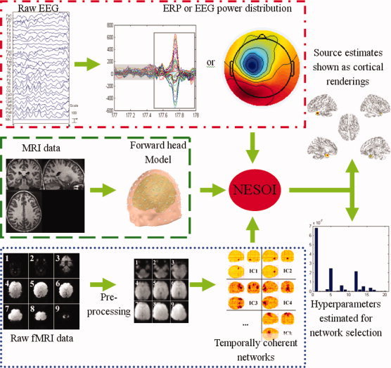
Schematic representation of NESOI. The raw EEG data is processed for artifact‐rejection and the amplitude and/or other features of interest are extracted. The corresponding fMRI data are pre‐processed and separated into spatially independent components. The structural MRI is segmented to provide a forward model for EEG imaging. The intensity of the neural electric sources and the hyperparameters are iteratively estimated by NESOI.

Establishment of forward head model (Green dashed border area in Fig. 1)

A high‐density canonical cortical mesh was extracted from the subject's structural MRI images. A lead‐field matrix was computed for the canonical mesh according to co‐registered electrode locations using a three‐sphere head model and routines from Fieldtrip software (http://fieldtrip.fcdonders.nl/download.php). The co‐registration and forward model was implemented with SPM8 (http://www.fil.ion.ucl.ac.uk/spm). This procedure provided a lead‐field matrix L ∈ R ^n×d coupling d cortical sources to n EEG electrodes, where each source has a unique location in the standard anatomical space of Talairach and Tournoux [1988].

Extraction of temporally coherent networks (Blue dotted border area in Fig. 1)

All functional images were realigned to the first functional image and time series of each slice were interpolated according to the acquisition time of the reference slice. Images were then spatially normalized to a standard EPI template. In total, k ICs (with waveforms and spatial maps) are estimated using the deflation approach of FastICA (http://www.cis.hut.fi/projects/ica/fastica/). Covariance components for EEG source imaging were constructed by the activated nodes of each IC using Eq. (6).

Preprocessing of EEG recordings (Red dash dotted border area in Fig. 1)

After artifact correction, EEG data is down‐sampled and band‐pass filtered. Temporal ICA is used for rejecting of the ballistocardiographic artifact and the residual MRI imaging artifact from the filtered EEG recordings if they are simultaneously recorded. Preprocessed EEG data are then utilized in the following source localization.

Estimation of EEG sources

ReML is used to estimate covariance hyperparameters at the source levels with covariance components derived from TCNs. Once these hyperparameters have been optimized, the posterior mean and covariance of the sources are then calculated with Eq. (8).

SIMULATION STUDY

In this section, we use simulated data to compare NESOI with other methods, giving an evaluation of the performance of the NESOI approach. We show the results in terms of four comparative metrics: localization error, temporal accuracy, explained variance, and model evidence. This section consists of four sub‐sections: an EEG forward model (including priors on the sources), simulated EEG data, evaluation metrics, and results.

Forward Model

The forward model in this simulation is derived from a high‐density canonical cortical mesh. These meshes were obtained by warping a template mesh to the T1‐weighted structural anatomy of an individual subject, as described in [Mattout et al., 2007]. This warping is the inverse of the transformation derived for the spatial normalization of the subject's structural MRI image. The calculation is a fully automated procedure established for other imaging modalities [Henson et al., 2009]. The template mesh is generated by Fieldtrip, and was extracted from a structural MRI of a neurotypical male. The wrapping procedure furnished a high‐density mesh with 33,001 vertices, which was uniformly distributed on the gray–white matter interface. Considering the computational load, the high‐density cortical surface was then down‐sampled to 6,557 vertices. Each vertex node is assumed to have one dipole, oriented perpendicular to the surface. The sensors were registered to the scalp surface, and the lead‐field matrix was calculated with SPM8 (http://www.fil.ion.ucl.ac.uk/spm). In this work, the utilized individual subject was from the single subject of the “multi‐modal face study” (available at http://www.fil.ucl.ac.uk/spm), whose data are further analyzed in Section “Multi‐modal Face Study.”

Simulated EEG Data

Using the real EEG data from the “multi‐modal face study,” we performed a singular value decomposition in sensor space to identify its principal time courses over time window of 800 ms (821 time bins with sampling rate of 1024 Hz), starting 200 ms before the presentation of a stimulus. We kept the first five singular vectors, T _θ ^5×821 and deployed them over five distributed sources or five TCNs. For each simulation, the five TCN sources in source space, S _θ ^6557×5, were randomly sampled from columns of the “6,557 × 20” Z‐score matrix W, which was generated using the method described in the above section “NEtworks SOurce Imaging (NESOI)” from the fMRI spatial ICA result of the “multi‐modal face study” (see Fig. 7). The assumed sources were projected through the lead‐fields to the sensor space as the simulated EEG signals by the transformation LS _θ T _θ. Temporal smoothed Gaussian noise was scaled to one‐tenth of the L ₁‐norm of the simulated signal. This provided a signal‐to‐noise ratio of ∼ 10. The signal and noise were then mixed to generate simulated data. An example of this procedure is shown in Figure 2. The procedure was repeated 256 times to give the average and standard deviation of the estimation metrics described in the following sub‐section.

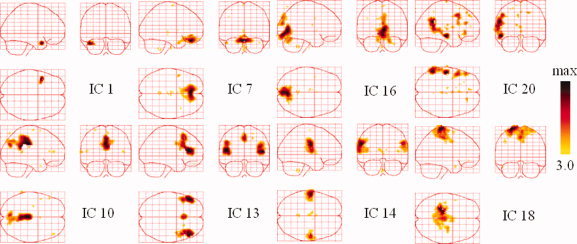
Figure 7.

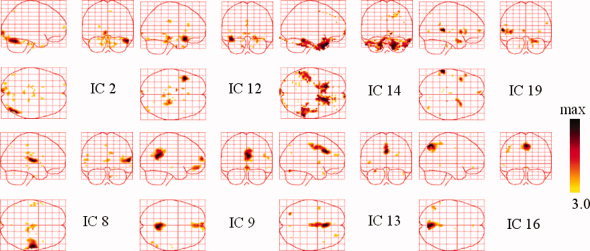
Temporally coherent networks of face perception revealed by ICs. Sagittal, coronal, and axial views of the spatial map are listed for each component. These are scaled to z scores and shown in a maximum intensity projection format. Yellow to black represent z values ranging from 3.0 to max. [Color figure can be viewed in the online issue, which is available at wileyonlinelibrary.com.]

Figure 2.

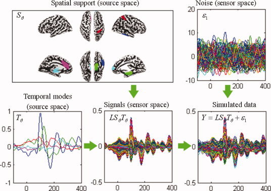
Schematic illustration of the construction of synthetic data. Upper left panel: five active sources distributed over nodes on the inflated cortical mesh (different colors). Lower left panel: the dynamics of these five sources derived from principal component decomposition of a real EEG recording. The color of the time course encodes the corresponding spatial support in the upper left panel. Lower middle panel: synthetic signals in sensor space obtained by projecting the signal in source space through the lead‐field matrix. Upper right panel: smoothed Gaussian noise. Lower right panel: simulated data generated by adding the smoothed Gaussian noise to the synthetic signal. Waveforms are shown between 100 ms before and 400 ms after stimulus onset. [Color figure can be viewed in the online issue, which is available at wileyonlinelibrary.com.]

Evaluation Metrics

The performance of the estimation was evaluated using localization error (LE), temporal accuracy (TA), explained variance (EV), and model evidence (ME). LE is defined as the mean geodesic distance between the assumed most active dipole over time bins and the estimated dipole with the largest conditional expectation over the same time bins; TA is defined as the squared correlation (i.e., the coefficient of determination) between the true time course of the assumed most active dipole and the conditional estimate used in assessing LE; EV is the fitted part of the data over all electrodes and time bins; ME is defined as the log of the marginal likelihood, and is approximated by F in Eq. (7).

Results

This procedure generated 256 synthetic datasets. Five inversions (MNM, LOR, dSPM, MSP, and NESOI) were implemented for each dataset. For dSPM and NESOI, the same five spatial priors were utilized (five columns in the activated matrix U derived from W). However, dSPM integrates all the priors into a single covariance component, whereas NESOI regards them as five components defined by Eq. (6).

Comparisons of five methods

In this section, to evaluate the methods in a situation that only part of the spatial priors derived from fMRI are the true source positions, S _θ, of EEG, we assumed that among the five spatial priors, five columns in U, only three were consistent with those in S _θ (i.e., that 60% of the priors were accurate, while the other two [40%], were the wrong priors). We implemented MNM, LOR, dSPM, MSP, and NESOI for 256 synthetic datasets. The results of the statistical analysis are shown in Figure 3.

Figure 3.

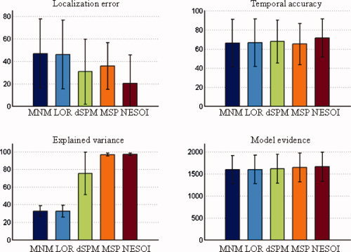
Mean value and standard deviation of the four evaluation metrics for the five methods: MNM, LOR, dSPM, MSP, and NESOI, respectively. Upper panels: Localization error (left) and temporal accuracy (right); lower panels: Explained variance (left) and model evidence (right). [Color figure can be viewed in the online issue, which is available at wileyonlinelibrary.com.]

Figure 3 (top left panel) illustrates that the estimations of the five approaches were stable with LE of less than 50 mm and TA larger than 50%. Moreover, despite the distinct features of the different approaches, NESOI consistently performed best in all four metrics.

Utilizing a partial concordance prior (60%), NESOI located the sources with mean spatial error of 20.28 mm. dSPM produced a mean error of 30.58 mm. These errors are both much smaller than those produced by the other “mono‐modality” methods, that is, MNM, LOR, and MSP, where only EEG information is used. MSP showed better performance than MNM and LOR, in line with previous studies [Friston et al., 2008; Henson et al., 2009]. Similarly, in terms of TA, the five approaches performed in the following order: NESOI>dSPM>LOR>MNM>MSP. Differences between the later four were small. In terms of EV, the differences among the five methods were distinct. In Figure 3 (bottom left panel), a relatively low proportion of the variance was explained by MNM, LOR, and dSPM (32.62%, 32.52%, and 75.23%, respectively). This may be because the source estimation was conducted upon all time bins. dSPM performed better than LOR and MNM in EV, but was highly unstable with standard deviation of 24.08%. In contrast, both MSP and NESOI explained almost all of the variances, explaining 96.54% and 96.84% of the variance, respectively. The variability of results from these methods over 256 realizations was also much smaller than the other three approaches.

Model evidence takes into account both data fit and model complexity [Friston et al., 2008]. In essence, it can be intuitively interpreted as an overall measure of the previous three metrics combined. Figure 3 (bottom right panel) shows very little difference in model evidence for the five approaches. However, setting aside the large baseline, the model evidence of NESOI (1655.92) was greater than the other four approaches (MNM: 1592.79, LOR: 1593.16, dSPM: 1608.97, MSP: 1640.70). This may be because NESOI is more flexible, integrating the benefits of both MSP and dSPM. In addition, LOR (1593.16) produced a better ME than MNM (1592.79), in accord with previous studies [Friston et al., 2008; Henson et al., 2009].

Comparison of dSPM and NESOI

Both dSPM and NESOI utilize functional information from fMRI recording. We sought to conduct a detailed comparison between the two techniques. In general, NESOI employs TCNs extracted by ICA, whereas dSPM utilizes SPM activation information extracted using the GLM. ICA and GLM are two different approaches for dealing with the spatial information from fMRI recording, which may influence corresponding EEG source localizations. However, the comparison between ICA and SPM was not the primary concern of our simulation, and we assumed that both dSPM and NESOI are based on the same priors. Thus, in this article we focus on possible differences due to the different construction of the prior matrices.

To reveal the quantitative differences between the dSPM and NESOI approaches more clearly, we designed six situations to mimic different levels of concordance/discordance between the EEG source space and the fMRI spatial priors. In the following implementation, all spatial priors were randomly sampled from U. The number of valid priors taken from the true source space, S _θ, however, were different. The simulations were also repeated 256 times, and the mean and standard deviation were obtained.

P0: perfect discordance. None of the five priors were from the spatial patterns in S _θ, that is, all priors were inaccurate;

P1–P4: mixed concordance. One to four of the spatial priors were from S _θ, that is, 20–80% of the priors were accurate for P1 to P4, respectively;

P5: perfect concordance. All the five priors were from S _θ.

The results of the statistical analysis are shown in Figure 4.

Figure 4.

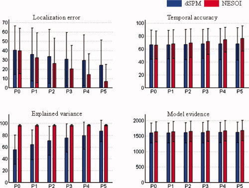
Mean value and standard deviation of evaluation metrics for dSPM and NESOI in different levels of concordance between EEG and fMRI. Upper panels: localization error (left) and temporal accuracy (right). Lower panels: explained variance (left) and model evidence (right). The number of valid priors varies from zero (P0) to five (P5), corresponding complete discordance or complete concordance between EEG and fMRI. [Color figure can be viewed in the online issue, which is available at wileyonlinelibrary.com.]

Figure 4 shows that the estimation performances of dSPM and NESOI increased steadily as the proportions of valid priors increased. Meanwhile, in all cases NESOI exhibited better performance than dSPM, especially for LA, EV, and ME. This difference may be due to the fact that NESOI assigns different hyperparameters for different priors. Thus, it may automatically prune redundant spatial priors, dSPM, in contrast, does not consider the possible difference among those priors, using the same weight for all priors.

Robustness of NESOI

In realistic conditions, typically only part of TCNs extracted from fMRI using ICA are related to the EEG signal. To investigate the effect of invalid priors on NESOI, in this simulation we assumed that the number of valid priors was fixed to three, while the number of invalid priors varied. The results of the statistical analysis of 256 runs are shown in Figure 5.

Figure 5.

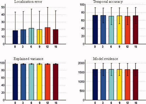
Mean value and standard deviation of evaluation metrics of NESOI. The number of valid priors is fixed at three, and the number of invalid priors is varied from 0 to 15. Upper panels: localization error (left) and temporal accuracy (right). Lower panels: explained variance (left) and model evidence (right). [Color figure can be viewed in the online issue, which is available at wileyonlinelibrary.com.]

Figure 5 shows that the influences of invalid priors can be ignored, because the performance of NESOI did not noticeably decrease as the number of invalid priors increased from zero to 15. Such robustness of NESOI may be due to the utilization of ReML to automatically select the reference priors. A study by Phillips et al. confirmed that the ReML solution was not measurably influenced by inaccurate priors, when accurate and inaccurate location priors were used simultaneously [Phillips et al., 2005]. Furthermore, using Monte‐Carlo simulations, similar results were also derived by Mattout et al. [2006]. The role of TCNs introduced in this work is similar to the location priors used in these previous studies, and NESOI is actually an extension of PEB framework by combing TCN priors. As such, NESOI shares the high robustness of PEB. This is particularly important for practical data, where the reliability of priors is typically not clear.

REAL DATA TEST

We used real data to further evaluate NESOI, in view of explained variance and model evidence. Two different datasets were used in this study. Dataset 1 was from a multimodal study on face perception and dataset 2 was collected from ac patient suffering from epilepsy.

Multi‐Modal Face Study

This dataset contains EEG and fMRI data from the same subject within the same paradigm, allowing a comparison between normal face images and scrambled face stimuli (for a detailed description of the paradigm, see [Henson et al., 2003] and http://www.fil.ion.ucl.ac.uk/spm, where the dataset can be downloaded).

fMRI/EEG acquisition and forward head model

EEG and fMRI were acquired separately in this study. A T1‐weighted structural MRI was acquired on a 1.5 T Siemens Sonata via an MDEFT sequence with resolution of 1 mm³. An EEG forward head model was established with the approach described in Section “Forward Model” by matching the T1‐weighted structural anatomy of the subject to the template. The T2‐weighted fMRI data was acquired using a Trajectory‐Based Reconstruction (TBR) gradient‐echo EPI sequence. There were 32 slices of 3 × 3 × 3 mm³ pixels, which were acquired in a sequential descending order with a TR of 2.88 s. EEG data were acquired with a 128‐sensor Active Two System with a sampling rate of 1024 Hz. Two electrodes on the left and right earlobe, as well as two other electrodes were used to measure HEOG and VEOG.

Preprocessing of EEG

The preprocessing of the EEG data included a re‐referencing to the average [Yao, 2001; Yao et al., 2005], and artifact rejection. Artifacts were defined as time‐points that exceeded an absolute threshold of 120 μV (these were found primarily in the VEOG). Eighty of the 344 trials were rejected due to artifacts in total. The differential ERP between faces and scrambled faces were then baseline‐corrected from −200 ms to 0 ms. The resulting ERP and its spatial distribution are shown in Figure 6. The ERPs exhibited an activity peak at 170 ms following stimulus onset, in accord with a face specific “N170” [Henson et al., 2003].

Figure 6.

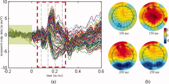
Differential ERPs for faces and scrambled faces. (a) Waveform of the ERPs, with a dashed rectangle depicting the actual time interval for analyzing. The scalp measurements exhibited a peak at 170 ms after stimulus onset. The signal masked by the green rectangle was used as a baseline. (b) Topographies of the differential ERPs at 100 ms, 150 ms, 200 ms, and 250 ms after stimulus onset. [Color figure can be viewed in the online issue, which is available at wileyonlinelibrary.com.]

Separation of temporally coherent networks

SPM8 was used for pre‐processing of fMRI data. Functional image time series data were first corrected for differences in slice acquisition times, then detrended, realigned with T1 volumes and warped into standard Talairach anatomical space. After dimension reduction using principal component analysis (PCA), 20 ICs with waveforms and spatial maps were estimated for the fMRI dataset using the deflation approach of the FastICA algorithm. The intensities of each spatial IC map were transformed to z scores. Those voxels with absolute z scores >3 were considered to be IC activated voxels. Some spatial maps in the 20 ICs are shown in Figure 7.

All 20 ICs were used in EEG source imaging, but Figure 7 only includes the ICs that are likely to be linked with brain function. The focally activated areas in the upper panels are likely to be related to face perception. IC2 exhibited a focal region around the right occipito‐temporal area (BA 19/22/39). IC12 showed a cluster around the left superior temporal pole region (BA 38). IC14 involved two bilateral pairs of the temporal fusiform gyrus and frontal rectal gyrus (BA 37/11). IC19 encompassed the left superior temporal gyrus (BA 42). The lower panels show components that resemble several resting state networks. IC8 involved the bilateral transverse temporal gyrus (BA 41/42), which areas widely considered to represent the auditory cortex. IC9 showed clusters of activity consisting of the prefrontal (BA 11), anterior cingulate (BA 32), posterior cingulate (BA 23/31), inferior temporal gyrus (BA 20/37), and superior parietal regions (BA 7). This pattern of brain regions is known as the default‐mode network, as described by Raichle et al. [2001]. IC13 showed activity in the posterior cingulate 86‐28‐83208238 (BA 23/31) regions, including the ventral anterior cingulate cortex (BA 33). These areas appear to be part of the default‐mode network shown in IC9. IC16 encompassed part of the extrastriate visual cortex in the occipital lobe (BA 18/19). These TCNs are highly correlated with the subject's state. As such, this information may be helpful for further EEG imaging. Other ICs did not have a clear relation with physiology, but may reflect various artifacts or noises and they are not listed in Figure 7. However, all 20 ICs (TCNs) were utilized in NESOI within a time window from 50 to 300 ms, because ReML can automatically select meaningful components and discard unrelated ones [Mattout et al., 2006; Philips et al., 2005]. The following results also confirmed this benefit of ReML.

Model comparison

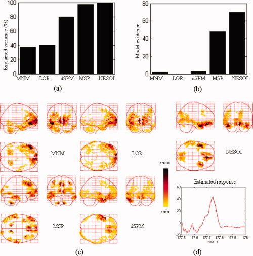
Having extracted TCNs, we then compared the five models of the previous section using the differential ERPs between faces and scrambled faces. The results are shown in Figure 8. These images showed 512 dipoles, with the greatest activity occurring at 170 ms.

Figure 8.

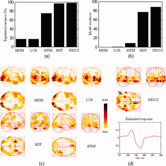
Model comparison among MNM, LOR, dSPM, MSP, and NESOI. (a) Explained variance; (b) Model evidence; (c) Maximum intensity projections of the spatial activities of face perception obtained by MNM, LOR, dSPM, and MSP; (d) The spatial profile and time course obtained by NESOI. [Color figure can be viewed in the online issue, which is available at wileyonlinelibrary.com.]

Both in terms of explained variance and model evidence, NESOI performed substantially better than any of the other models. Meanwhile, the results confirmed that the spatially coherent model (LOR) outperformed the classical minimum norm (MNM), although this performance difference was relatively small. The reconstructed profile of MNM was substantially more superficial and dispersed. The activations revealed by MNM were mainly located in the bilateral inferior and middle temporal gyrus (BA 17/18). LOR exhibited an additional activated area in the inferior temporal gyrus (BA 37) that was not shown by MNM. Two activated areas located in the right fusiform gyrus and medial frontal area were revealed by dSPM. This result is consistent with the fMRI SPM result shown in the right panel of Figure 9. However, it is difficult to relate these sources to the negative area in the left occipital region (see topography at 200 ms after stimulus onset in Fig. 6b). With 256 components per hemisphere (i.e., 768 = 3 × 256 components in all), MSP revealed activity in bilateral middle and superior temporal gyrus (BA 21/38). The results of the MSP inversion are partially consistent with MNM and LOR, but the deep and frontal sources (BA 21/38) were revealed more clearly. The sources estimated by NESOI (Fig. 8d) were similar to the results of dSPM, which shown two strongly activated areas in the right temporal lobe and a medial frontal area (Talairach coordinates: 12, 34, −16 mm). The time course in the right temporal lobe exhibited an activity peak at 170 ms, suggesting that this region may be related to the N170. Two activated areas in the right temporal lobe were located in the right fusiform gyrus of the temporal lobe with Talairach coordinates (34, −48, −13 mm) and in the right superior temporal gyrus with Talairach coordinates (62, −31, 12 mm), respectively. These N170 related regions are consistent with the profile reported in a previous study of brain activation measured in a group of eighteen subjects using fMRI SPM [Henson et al., 2003]. A weak source in the left fusiform gyrus was found by NESOI, shown in Figure 8d (indicated by arrow). This area may be a source accounting for the negative left occipital potential. dSPM did not reveal activation in this area. In summary, compared with the other four methods, NESOI indicated much stronger activations in the right fusiform gyrus and medial frontal area, and a weak source in left fusiform. These results are consistent with both the scalp potential map (Fig. 6b) and the following fMRI SPM result (Fig. 9 right panel).

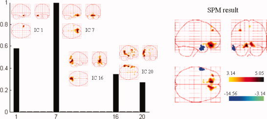
Figure 9.

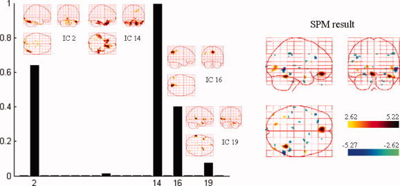
Spatial components that were automatically selected by NESOI and the fMRI SPM result for the same subject. Left panel: Hyperparameter γ_i estimated for each TCN. IC2, IC14, IC16, and IC19 were selected with support from EEG data having relatively larger hyperparameters. Right panel: SPM statistical result of the same subject within the same paradigm. [Color figure can be viewed in the online issue, which is available at wileyonlinelibrary.com.]

The left panel of Figure 9 shows four ICs that were automatically selected based on the estimated hyperparameter for each IC, to further examine the NESOI procedure. The networks related to IC2, 14, 16, and 19 were supported by the EEG data. These networks showed relatively larger hyperparameters. As such, these networks are likely to be relevant to the different physiological procedures of faces versus scrambled faces. The fMRI SPM of the same subject is also shown in the right panel of Figure 9. Among these four ICs, IC14 involves a bilateral activation in the frontal gyrus (BA 11), close to the positive active cluster indicated by SPM. IC2 contains a region that is overlapped by a negatively active area from the SPM analysis. Because it uses the priors of SPM, dSPM produced very similar results to the SPM analysis. For NESOI (Fig. 8d), although the main findings were the same as the fMRI SPM result (Fig. 9 right panel), they were not entirely the same as the pattern indicated by ICs 16 and 19. This suggests that the integration of EEG and fMRI does indeed provide mutually complementary information [Shmuel et al., 2006].

Regions Involved in Epileptic Discharges

Study protocol and patient

A 10‐year‐old right‐handed male patient with epilepsy participated in an EEG‐fMRI study in the epilepsy clinic of the West China Hospital of Neurology, Sichuan University. Informed consent was obtained before the patient underwent a clinical brain structural MRI and a 24‐h video EEG. A diagnosis was established according to the scheme published by the International League against Epilepsy in 2001 [Engel, 2001]. This patient experienced a seizure at 9 years of age, and was treated with sodium valproate. He was diagnosed as suffering from complex partial seizures, and secondary generalized tonic‐clonic seizures. Twenty‐four‐hour VEEG revealed ictal discharges in the bilateral temporal and frontal lobes. A clinical structural MRI of the brain revealed an anatomical abnormality, with an enlarged cisterna magna. Interictal EEG revealed bilaterally paroxysmal spike waves and spike‐slow‐waves over the fronto‐temporal parietal and occipital regions [Luo et al., 2010].

EEG and fMRI were simultaneously recorded for 4 min. The patient was instructed to simply lie inside the scanner with eyes closed. He was also required to keep awake during the experiment. No visual or auditory stimuli were presented at any time during the functional scanning.

MRI/fMRI acquisition and forward head model

Functional images were acquired with a 3T MRI scanner (EXCITE, GE Milwaukee, USA) using means of T2*‐weighted echo planar imaging free induction decay sequences with the following parameters: echo time (TE) of 30 ms; matrix size of 64 × 64; field of view (FOV) of 240 mm × 240 mm; in‐plane voxel size of 3 × 3 mm²; flip angle of 90°; slice thickness of 5 mm; and no gap. Functional volumes consisted of 30 bicommissural slices, which were acquired with a volume repeat time (TR) of 2 s. A total of 205 volumes were acquired, and the first five volumes were discarded to ensure steady‐state longitudinal magnetization. Subsequently, a high‐resolution T1‐weighted structural volume was acquired via a 3D spoiled gradient recalled (SPGR) sequence with the following parameters: thickness of 1 mm (no gap); TR of 8.5 ms; TE of 3.4 ms; FOV of 240 mm × 240 mm; flip angle of 12°; and a matrix of 512 × 512. The high‐resolution T1‐weighted structural volume provided an anatomical reference for the functional scan and the forward model of EEG imaging. The forward head model is established with the same method described by matching the T1‐weighted structural anatomy of the patient to the template.

EEG acquisition and preprocess

An MR‐compatible Mizar 40 system (EBNeuro, Florence, Italy) was used for EEG recordings with 32 electrodes. All electrodes were ring‐type sintered nonmagnetic Ag/AgCl electrodes, placed on the scalp according to the international 10/20 system. An additional electrode was dedicated to the electrocardiogram (ECG). Two other electrodes were positioned over the subject's earlobes, with their average used as a reference. The impedance of each electrode was maintained below 5 kΩ using electrode paste. Data were collected with a sampling rate of 4096 Hz, and band‐pass filtering from 0.016 to 250 Hz was applied.

The BE‐MRI Toolbox (Galileo New Technology, Florence, Italy) was used for offline correction of the MRI imaging artifact. This software implements the adaptive artifact subtraction (AAS) method, in which the MRI imaging artifact waveforms are segmented, averaged, and iteratively subtracted from the EEG signals [Allen et al., 2000]. Subsequently, data were down‐sampled to 1 kHz and digitally filtered within the 1–50 Hz frequency band using a Chebyshev II‐type filter with 40 dB attenuation and zero‐phase distortion. After visually checking for movement artifacts and noisy electrodes from the data, a method based on temporal ICA was used to reject the ballistocardiographic (BCG) artifact and the residual imaging artifact from the filtered EEG recordings [Mantini et al., 2009]. Figure 10 illustrates the EEG signal before and after artifact correction.

Figure 10.

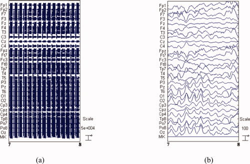
Raw EEG and artifact‐removed EEG. (a) 1 s raw EEG data collected during simultaneous EEG/fMRI, (b) the same traces after band‐pass filtering and image artifact attenuation using AAS. [Color figure can be viewed in the online issue, which is available at wileyonlinelibrary.com.]

The EEG data was analyzed by an experienced neurophysiologist. This expert selected a suitable typical electrode and used the raw EEG data to identify interictal epileptic discharges (IEDs) and mark the times of IED. Bipolar recordings (Fig. 11a) revealed a typical IED between 177.7 s and 177.8 s. With the topographies (Fig. 11b), the potential of the left hemisphere increased from 177.6 s, reached a maximum at 177.7 s and returned to normal at 177.8 s. In the right hemisphere, a positive potential appeared at 177.6 s, then turned to a negative potential at 177.7 s. The potential eventually returned to ∼ 0.

Figure 11.

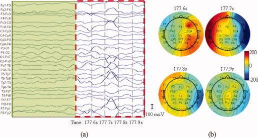
Epileptic discharges recorded on the scalp in an MR scanner. (a) Waveform of the discharge. The dashed rectangle signal contained the clinic typical IEDs that were selected by a clinical expert and the signal masked by the green rectangle is used as a baseline. (b) Topographies of the discharges at 177.6 s, 177.7 s, 177.8 s, and 177.9 s during the acquisition of the functional images. [Color figure can be viewed in the online issue, which is available at wileyonlinelibrary.com.]

Separation of temporally coherent networks

TCNs were extracted with the same method described in Section “Model Comparison.” Figure 12 shows TCNs that we considered likely to be linked with known brain networks.

Figure 12.

Resting state networks from a patient with epilepsy. The sagittal, coronal, and axial views of the spatial map are shown. They are scaled to z scores and shown in maximum intensity projection format. Yellow to black represent the range of z values from 3.0 to max. [Color figure can be viewed in the online issue, which is available at wileyonlinelibrary.com.]

The SPM evidence shown in the right panel of Figure 14 suggests that the focally activated areas in the upper panels may be related to epilepsy. IC1 exhibited a focally activated region around the left temporal region, which is at least partially compatible with the positive peaks in the EEG topography at 177.7 s (Fig. 11b). The components illustrated in the lower panels reveal several fundamental TCNs. IC10 showed a cluster of activity, consisting of the posterior cingulate (BA 23/31) and the superior parietal (BA 7) regions, both of which are considered to be part of the default‐mode network [Raichle et al., 2001]. IC14 implicated the superior temporal (BA 22), insular, and postcentral cortices (BA 1/2), which represent the auditory cortex. IC16 encompasses part of the striate and parastriate regions (BA 17/18) belonging to the visual cortex. IC18 shows the pre‐ and post‐central gyri (BA 1/2/3/4) correlated with the motor and sensory networks. Other ICs that we considered to correspond to noise and artifacts are not shown in Figure 12. The results revealed that most of the obtained TCNs were highly correlated with the patient's state. As such, they may be helpful in facilitating EEG imaging.

Figure 14.

Spatial components automatically selected by NESOI and the fMRI SPM from the same subject. Left panel: Hyperparameter γ_i estimated for each TCN. IC1, IC7, IC16, and IC20 are selected with support from EEG data, having relatively larger hyperparameters. Right panel: EEG‐informed SPM result of the same patient. [Color figure can be viewed in the online issue, which is available at wileyonlinelibrary.com.]

Model comparison

The sources of discharges estimated by MNM, LOR, dSPM, MSP, and NESOI are shown in Figure 13. These images show the 512 dipoles exhibiting the greatest activity during the spike discharge.

Figure 13.

Model comparison between MNM, LOR, dSPM, MSP, and NESOI models. (a) Explained variance; (b) Model evidence; (c) Maximum intensity projections of the spatial activities of epileptic discharges obtained by MNM, LOR, dSPM, and MSP; (d) The spatial profile and time course obtained by NESOI. [Color figure can be viewed in the online issue, which is available at wileyonlinelibrary.com.]

Figure 13a,b shows that NESOI has the best performance among the five models in view of explained variance and model evidence. The MNM and LOR localized sources in similar areas, although the reconstructed profiles of MNM were more superficial. dSPM localized sources in bilateral frontal and left temporal lobes. These sources are consistent with the SPM result shown in the right panel of the following Figure 14. However, the sources accounting for the negative peak in right hemisphere of Figure 11b were not indicated by LOR, MNM, or dSPM. In MSP, 128 components per hemisphere selected by log‐evidence were evenly sampled from the coherence matrix in (4). The maximum intensity projections indicated some dispersed activated regions using the MSP and NESOI approaches. Specifically, MSP revealed bilateral pairs of fusiform gyrus and inferior frontal gyrus activity, in conjunction with a ventral prefrontal source. In contrast, NESOI revealed three focally activated areas, corresponding to the bilateral frontal and temporal lobes. The results of the NESOI approach are in accord with the topography in Figure 11b, and are largely consistent with the EEG‐informed GLM using IEDs as regressors (see right panel, Fig. 14). Importantly, the results revealed a right temporal source that was missed by dSPM, but retrieved by NESOI. Right temporal lobe activity does not appear in any network extracted from fMRI (see Fig. 12), meaning that the fMRI priors utilize in NESOI did not involve information about this area. This is entirely different from the case of the data from the “multi‐modal face study,” where ICA retrieved all the source priors. When the fMRI spatial patterns provide only part of the prior information required by NESOI, the multiple sparse priors evenly sampled from the residual source space may supplement the missed priors. This allows NESOI to reconstruct sources missed by fMRI. Though the right temporal lobe source identified by NESOI is not revealed by fMRI measurements, it is compatible with the IED revealed by the scalp EEG over the right temporal lobe (see topographies at 177.6 s and 177.7 s in Fig. 11b). Further check the sign of source reveals that the directions of dipoles in the two hemispheres are reversed (the detailed figures omitted), they may indicate an activation and contralateral inhibition pattern, which is consistent with the topography at 177.7 s (Fig. 11b). The other four methods, in contrast, did not detect strong activation in the right temporal lobe.

The hyperparameters estimated with NESOI are shown in the left panel of Figure 14, and the EEG‐informed fMRI SPM statistical results for this patient are shown in the right panel. For EEG‐informed fMRI, the canonical HRF was convolved with IED time pulse function as a regressor of interest in the SPM design matrices. Six parameters for spatial realignment were included to model the linear and non‐linear effects of head motion. Design matrices and data were high‐pass filtered with a cutoff of 128 s. The specifically activated areas were calculated using statistical t‐tests with five contiguous voxels above an absolute t value of 3.14 (P < 0.001, uncorrected). Networks related to IC1, IC7, IC16, and IC20 were in accord with the EEG data showing larger hyperparameters, indicating that these networks may be relevant to the patient's epileptic discharges. IC7 involved the bilateral inferior frontal gyrus (BA 11), largely consistent with the areas of positive activation indicated in the fMRI SPM result. IC1 indicated a region close to the negatively active area revealed by the fMRI SPM result.

DISCUSSION

To investigate the relationship between the scalp surface electrical features and the fMRI spatial maps, in this study we developed a completely data‐driven approach, NESOI, combining high‐resolution spatial information from fMRI recording, with high‐resolution temporal information from EEG recording, in an effort to increase the accuracy of source estimation methods. Our NESOI approach uses ICA to identify multiple, widely distributed temporally coherent networks from fMRI data. Networks are then used as covariance components of PEB for EEG imaging. The major novel feature of this approach is the utilization of multiple temporally coherent priors and the automatic selection of fMRI brain networks supported by EEG.

A large number of algorithms based on neuronal‐anatomical priors have been previously reported. These approaches have used spatially based priors derived from MRI spatial information [Phillips et al., 2002], an assumption that neighboring nodes exhibit similar neuronal activity [Friston et al., 2008; Pascual‐Marqui, 2002], or activation priors derived from fMRI statistical analysis [Dale et al., 2000; Daunizeau et al., 2005; Liu et al., 1998]. In our new NESOI approach, temporally coherent networks in the brain, including networks found during a resting state and those active during cognitive tasks, were utilized in EEG source imaging. This current comparative study indicated that this novel method can produce physiologically reasonable results. The main benefits of the NESOI approach over other techniques are related to two basic features of the method. First, NESOI uses ICA to extract temporally coherent network priors from fMRI. Previous investigations have confirmed that for fMRI data, ICA processes a significant advantage over the widely used GLM approach, because it does not require a priori specification of activation waveforms, and can identify similar loci of task‐related activation [Calhoun et al., 2009]. Therefore, NESOI can use more flexible spatial priors than its closest competitor, dSPM, which is based on the GLM model. This advantage is illustrated by the results of the “multi‐modal face study” that we used as a test case. For this data set, analysis with the prior IC14 revealed activation in bilateral fusiform gyri (see Fig. 7). NESOI indicated symmetric sources in these areas. In contrast, SPM revealed no source in the left fusiform gyrus (Fig. 9 right panel), meaning that dSPM also neglected this source. Second, NESOI adopts PEB analysis to estimate source parameters as well as their spatial covariances, meaning that both multiple sparse priors and fMRI functional networks are utilized. The framework in the NESOI approach can adapt to different levels of concordance between EEG and fMRI. In addition to the simulation results (Figs. 2, 3, 4), applying the NESOI approach to data from a patient suffering from epilepsy also confirmed the potential of our method. The results revealed that NESOI was able to retrieve activations in the right temporal lobe that were not found in fMRI recording. Future research using intracranial EEG would be useful for further evaluating the utility of this novel method and assessing its validity [Ebersole et al., 1996].

Previous research has reported that ReML can automatically select the reference priors. Phillips et al. [2005] affirmed that when accurate and inaccurate location priors were used simultaneously, the solution was not obviously influenced by the inaccurate information. Except for the use of temporally coherent networks as priors, the PEB frameworks used in the NESOI approach are the same as those used in Phillips et al. [2005]. The comparison of the NESOI method with four other inversion schemes in a series of simulation studies further confirms that the effects of inaccurate priors on source estimation using NESOI are negligible, provided accurate priors are also provided (see Fig. 4). Friston et al. [2008] showed that a Laplace approximation to the posterior of the hyperparameters makes it possible to quickly and efficiently invert models with multiple priors. In all of these methods, the Automatic Relevance Determination (ARD) is an essential component. In fact, ReML can be used to optimally determine the marginal likelihood or evidence. This is useful for model selection, because the hyperpriors can force the conditional variance of hyperparameters to approach zero when their conditional mean is zero. In short, ReML can be used to estimate the hyperparameters that control mixtures of covariance components in a source space that generates the data. If there are redundant functional network priors, ReML will automatically switch them off or suppress them to provide a forward model with the greatest evidence or marginal likelihood. The NESOI, MSP, and LOR methods all are examples of ARD, referring to a general phenomenon in hierarchical Bayesian models where maximizing evidence enables the pruning away of unnecessary model components [see Neal, 1996]. Though some previous empirical reports [Friston et al., 2008; Henson et al., 2009] and the current results indicate that the Laplace approximation of the model evidence F can be very informative in practice, it should be noted that the current approximation could potentially distort the results of the model selection. The Laplace approximation, however, can be ameliorated by combining the Laplace and mean‐field approximations [Wipf and Nagarajan, 2009].

To infer TCNs from the fMRI time series for PEB based EEG source imaging, most previous studies have applied a region‐of‐interest (ROI) cross‐correlation analysis approach [Hampson et al., 2004], where the spatial patterns of similar fluctuations are estimated by correlation analysis against a reference time course derived from a seeded voxel. The networks extracted by this method can also be used in the NESOI method. However, the result is ROI dependent. In the current study, we adopted the much simpler and more convenient ICA approach to extract these networks. Generally, each component corresponds to a certain functional brain network. These component‐determined networks may provide valuable complementary information useful for EEG source localization. It has been established that the IC component selection is the primary problem for the application of ICA to fMRI analysis. For our new method, all TCNs are used as priors and included in ReML inversion. When there is displacement between a BOLD activation networks and an electrophysiological source, a nearby deactivation network may bias electrical activity estimates. However, it should be noted that we have never observed such a case in practice. Including TCNs with clear physiological meaning could potentially ameliorate this possible problem.

Any attempt at combining information of EEG and fMRI inevitably encounters the problem that EEG and fMRI measurements may be due to different physiological processes. fMRI measures changes in blood oxygen level, which is simultaneously affected by blood volume, flow rate, and the oxygen content of the blood. The various factors that contribute to the BOLD signal can be directly or indirectly related to the metabolism of brain cells and, thus, neural activity. The currents generating EEG, on the other hand, are dependent on ionic activity. These electrophysiological signals are produced when neuronal activity causes alterations in the flow of ions into and out of neurons. Currents are roughly synchronous with and proportional to activity. In addition, the current is fundamentally a vector, but its divergence is a scalar. Therefore, it is possible to describe EEG sources using an equivalent charge model [Lei et al., 2009b; Xu et al., 2008; Yao, 1996] or by an equivalent dipole model, as we have adopted in the current study. Several previous studies have shown that the BOLD signal and neural activity are correlated. Moreover, it has been shown that if the frequency of the neural activity is fixed, the BOLD signal is roughly linearly proportional to the neural activity [Heeger et al., 2000; Shmuel et al., 2006]. The BOLD signal has also been shown to be proportional to local field potentials [Shmuel et al., 2006]. As the current sources (and local field potentials) would expect to be proportional to neural activity, it is reasonable to expect the sources of the EEG signal to be proportional to the BOLD signal. This is the basis of the logic behind our inverse scheme, in which the modes of TCN obtained from fMRI recording are added as variance of current density to ensure that the variance of the EEG imaging solution is proportional to the BOLD signal. Dipoles with same variance can have different mean values, and their direction can be very different from each other. It should be noted, however, that variances only control the possibility that a dipole will be an active source.

CONCLUSION

The results of the current study revealed that our novel NESOI approach was able to produce a realistic solution by combining the high temporal resolution of EEG and the high spatial resolution of fMRI. We successfully used the resulting hyperparameters to indicate which spatial patterns were supported by EEG data. Task‐related temporally coherent networks can be automatically selected according to these hyperparameters at the same time [Lei et al., 2010]. Moreover, this method is immune to the temporal dissimilar modalities of EEG and fMRI. The current findings provide a helpful framework for our future research, which will focus on the relationship between endogenous brain oscillations and related networks.

REFERENCES

- Ahlfors SP, Simpson GV, Dale AM, Belliveau JW, Liu AK, Korvenoja A, Virtanen J, Huotilainen M, Tootell RB, Aronen HJ, Ilmoniemi RJ ( 1999): Spatiotemporal activity of a cortical network for processing visual motion revealed by MEG and fMRI. J Neurophysiol 82: 2545–2555. [DOI] [PubMed] [Google Scholar]
- Allen PJ, Josephs O, Turner R ( 2000): A method for removing imaging artifact from continuous EEG recorded during functional MRI. NeuroImage 12: 230–239. [DOI] [PubMed] [Google Scholar]
- Auranen T, Nummenmaa A, Vanni S, Vehtari A, Hämäläinen MS, Lampinen J, Jääskeläinen IP ( 2009): Automatic fMRI‐guided MEG multidipole localization for visual responses. Hum Brain Mapp 30: 1087–1099. [DOI] [PMC free article] [PubMed] [Google Scholar]
- Beckmann CF, DeLuca M, Devlin JT, Smith SM ( 2005): Investigations into resting‐state connectivity using independent component analysis. Philos Trans R Soc Lond B Biol Sci 360: 1001–1013. [DOI] [PMC free article] [PubMed] [Google Scholar]
- Bénar CG, Gross DW, Wang Y, Petre V, Pike B, Dubeau F, Gotman J ( 2002): The BOLD response to interictal epileptiform discharges. Neuroimage 17: 1182–1192. [DOI] [PubMed] [Google Scholar]
- Calhoun VD, Liu J, Adalı T ( 2009): A review of group ICA for fMRI data and ICA for joint inference of imaging, genetic, and ERP data. NeuroImage 45: S163–S172. [DOI] [PMC free article] [PubMed] [Google Scholar]
- Chen H, Yao D ( 2004): Discussion on the choice of separated components in fMRI data analysis by spatial independent component analysis. Magn Reson Imag 22: 827–833. [DOI] [PubMed] [Google Scholar]
- Dale AM, Liu AK, Fischl BR, Buckner RL, Belliveau JW, Lewine JD, Halgren E ( 2000): Dynamic statistical parametric mapping: Combining fMRI and MEG for highresolution imaging of cortical activity. Neuron 26: 55–67. [DOI] [PubMed] [Google Scholar]
- Dale AM, Halgren E ( 2001): Spatiotemporal mapping of brain activity by integration of multiple imaging modalities. Curr Opin Neurobiol 11: 202–208. [DOI] [PubMed] [Google Scholar]
- D'Argembeau A, Collette F, Van der Linden M, Laureys S, Del Fiore G, Degueldre C, Luxen A, Salmon E ( 2005): Self‐referential reflective activity and its relationship with rest: A PET study. NeuroImage 25: 616–624. [DOI] [PubMed] [Google Scholar]
- Daunizeau J, Grova C, Mattout J, Marrelec G, Clonda D, Goulard B, Lina JM, Benali H ( 2005): Assessing the relevance of fMRI‐based prior in the EEG inverse problem: A Bayesian model comparison approach. IEEE Trans Signal Process 53: 3461–3472. [Google Scholar]
- Disbrow EA, Slutsky DA, Roberts TP, Krubitzer LA ( 2000): Functional MRI at 1.5 tesla: a comparison of the blood oxygenation level‐dependent signal and electrophysiology. Proc Natl Acad Sci USA 97: 9718–9723. [DOI] [PMC free article] [PubMed] [Google Scholar]
- Ebersole JS, Pacia SV ( 1996): Localization of temporal lobe foci by ictal EEG patterns. Epilepsia 37: 386–399. [DOI] [PubMed] [Google Scholar]
- Engel J Jr ( 2001): A proposed diagnostic scheme for people with epileptic seizures and with epilepsy: Report of the ILAE task force on classification and terminology. Epilepsia 42: 796–803. [DOI] [PubMed] [Google Scholar]
- Friston KJ, Penny W, Phillips C, Kiebel S, Hinton G, Ashburner J ( 2002): Classical and Bayesian inference in neuroimaging: Theory. NeuroImage 16: 465–483. [DOI] [PubMed] [Google Scholar]
- Friston KJ, Mattout J, Trujillo‐Barreto N, Ashburner J, Penny W ( 2007): Variational free energy and the Laplace approximation. NeuroImage 34: 220–234. [DOI] [PubMed] [Google Scholar]
- Friston KJ, Harrison L, Daunizeau J, Kiebel S, Phillips C, Trujillo‐Barreto N, Henson R, Flandin G, Mattout J ( 2008): Multiple sparse priors for the MEG/EEG inverse problem. NeuroImage 39: 1104–1120. [DOI] [PubMed] [Google Scholar]
- Gerloff C, Grodd W, Altenmüller E, Kolb R, Klose TNU, Voigt K, Dichgans J ( 1996): Coregistration of EEG and fMRI in a simple motor task. Hum Brain Mapp 4: 199–209. [DOI] [PubMed] [Google Scholar]
- Goldman RI, Stern JM, Engel J Jr, Cohen MS ( 2002): Simultaneous EEG and fMRI of the alpha rhythm. NeuroReport 13: 2487–2492. [DOI] [PMC free article] [PubMed] [Google Scholar]
- Hampson M, Olson IR, Leung HC, Skudlarski P, Gore JC ( 2004): Changes in functional connectivity of human MT/V5 with visual motion input. NeuroReport 15: 1315–1319. [DOI] [PubMed] [Google Scholar]
- Harrison LM, Penny W, Ashburner J, Trujillo‐Barreto N, Friston KJ ( 2007): Diffusion‐based spatial priors for imaging. NeuroImage 38: 677–695. [DOI] [PMC free article] [PubMed] [Google Scholar]
- Heeger DJ, Huk AC, Geisler WS, Albrecht DG ( 2000): Spikes versus bold: What does neuroimaging tell us about neuronal activity? Nat Neurosci 3: 631–633. [DOI] [PubMed] [Google Scholar]
- Henson RN, Goshen‐Gottstein Y, Ganel T, Otten LJ, Quayle A, Rugg MD ( 2003): Electrophysiological and hemodynamic correlates of face perception, recognition and priming. Cereb Cortex 13: 793–805. [DOI] [PubMed] [Google Scholar]
- Henson RN, Mattout J, Phillips C, Friston KJ ( 2009): Selecting forward models for MEG source‐reconstruction using model‐evidence. NeuroImage 46: 168–176. [DOI] [PMC free article] [PubMed] [Google Scholar]
- Hyvärinen A, Oja E ( 1997): A fast fixed‐point algorithm for independent component analysis. Neural Comput 9: 1483–1492. [DOI] [PubMed] [Google Scholar]
- Jacobs J, Hawco C, Kobayashi E, Boor R, LeVan P, Stephani U, Siniatchkin M, Gotman J ( 2008): Variability of the hemodynamic response as a function of age and frequency of epileptic discharge in children with epilepsy. NeuroImage 40: 601–614. [DOI] [PMC free article] [PubMed] [Google Scholar]
- Lei X, Yao D ( 2009): EEG source localization based on multiple fMRI spatial patterns. The Second International Conference on Cognitive Neurodynamics. Hangzhou, China.
- Lei X, Yang P, Yao D ( 2009a): An empirical Bayesian framework for brain computer interfaces. IEEE Trans Neural Syst Rehab Eng 17: 521–529. [DOI] [PubMed] [Google Scholar]
- Lei X, Chen A, Xu P, Yao D ( 2009b). Gaussian source model based iterative algorithm for EEG source imaging. Comput Biol Med 39: 978–988. [DOI] [PubMed] [Google Scholar]
- Lei X, Qiu C, Xu P, Yao D ( 2010): A parallel framework for simultaneous EEG/fMRI analysis: Methodology and simulation. NeuroImage 52: 1123–1134. [DOI] [PubMed] [Google Scholar]
- Liu AK, Belliveau JW, Dale AM ( 1998): Spatiotemporal imaging of human brain activity using functional MRI constrained magnetoencephalography data: Monte Carlo simulations. Proc Natl Acad Sci USA 95: 8945–8950. [DOI] [PMC free article] [PubMed] [Google Scholar]
- Luo C, Li Q, Xia Y, Lai Y, Qin Y, Liao W, Zhou D, Yao D, Gong Q: Altered functional connectivity in default mode network in absence epilepsy: A resting‐state fMRI study. Hum Brain Mapp (in press). [DOI] [PMC free article] [PubMed] [Google Scholar]
- Mantini D, Corbetta M, Perrucci MG, Romani GL, Gratta CD ( 2009): Large‐scale brain networks account for sustained and transient activity during target detection. NeuroImage 44: 265–274. [DOI] [PMC free article] [PubMed] [Google Scholar]
- Mattout J, Phillips C, Penny W, Rugg MD, Friston KJ ( 2006): MEG source localization under multiple constraints: An extended Bayesian framework. NeuroImage 30: 753–767. [DOI] [PubMed] [Google Scholar]
- Mattout J, Henson RN, Friston KJ ( 2007): Canonical source reconstruction for MEG. computational intelligence and neuroscience. Article ID:67613. [DOI] [PMC free article] [PubMed]
- McKeown MJ, Makeig S, Brown GG, Jung TP, Kindermann SS, Bell AJ, Sejnowski TJ ( 1998): Analysis of FMRI data by blind separation into independent spatial components. Hum Brain Mapp 6: 160–188. [DOI] [PMC free article] [PubMed] [Google Scholar]
- Moosmann M, Eichele T, Nordby H, Hugdahl K, Calhoun VD ( 2008): Joint independent component analysis for simultaneous eeg‐fmri: Principle and simulation. Int J Psychophysiol 67: 212–221. [DOI] [PMC free article] [PubMed] [Google Scholar]
- Neal RM ( 1996): Bayesian Learning for Neural Networks. New York: Springer‐Verlag; 205 p. [Google Scholar]
- Pascual‐Marqui RD ( 2002): Standardized low‐resolution brain electromagnetic tomography (sLORETA): Technical details. Methods Find Exp Clin Pharmacol 24: 5–12. [PubMed] [Google Scholar]
- Phillips C, Rugg MD, Friston KJ ( 2002): Anatomically informed basis functions for EEG source localization: Combining functional and anatomical constraints. NeuroImage 16: 678–695. [DOI] [PubMed] [Google Scholar]
- Phillips C, Mattout J, Rugg MD, Maquet P, Friston KJ ( 2005): An empirical Bayesian solution to the source reconstruction problem in EEG. NeuroImage 24: 997–1011. [DOI] [PubMed] [Google Scholar]
- Raichle ME, MacLeod AM, Snyder AZ, Powers WJ, Gusnard DA, Shulman GL ( 2001): A default mode of brain function. Proc Natl Acad Sci USA 98: 676–682. [DOI] [PMC free article] [PubMed] [Google Scholar]
- Sato MA, Yoshioka T, Kajihara S, Toyama K, Goda N, Doya K, Kawato M ( 2004): Hierarchical Bayesian estimation for MEG inverse problem. NeuroImage 23: 806–826. [DOI] [PubMed] [Google Scholar]
- Scheeringa R, Petersson KM, Oostenveld R, Norris DG, Hagoort P, Bastiaansen MCM ( 2009): Trial‐by‐trial coupling between EEG and BOLD identifies networks related to alpha and theta EEG power increases during working memory maintenance. NeuroImage 44: 1224–1238. [DOI] [PubMed] [Google Scholar]
- Shmuel A, Augath M, Oeltermann A, Logothetis NK ( 2006): Negative functional mri response correlates with decreases in neuronal activity in monkey visual area v1. Nat Neurosci 9: 569–577. [DOI] [PubMed] [Google Scholar]
- Stancák A, Polácek H, Vrána J, Rachmanová R, Hoechstetter K, Tintra J, Scherg M ( 2005): Eeg source analysis and fmri reveal two electrical sources in the frontoparietal operculum during subepidermal finger stimulation. NeuroImage 25: 8–20. [DOI] [PubMed] [Google Scholar]
- Talairach J, Tournoux P ( 1988): Co‐Planar Stereotaxic Atlas of the Human Brain. Germany: Thieme, Stuttgart; 122 p. [Google Scholar]
- Tikhonov AN, Arsenin VY ( 1977): Solutions of Ill‐Posed Problems. New York: John Wiley; 258 p. [Google Scholar]
- Trujillo‐Barreto N, Aubert‐Vazquez E, Valdes‐Sosa P ( 2004): Bayesian model averaging. NeuroImage 21: 1300–1319. [DOI] [PubMed] [Google Scholar]
- Whittingstall K, Stroink G, Schmidt M ( 2007): Evaluating the spatial relationship of event‐related potential and functional mri sources in the primary visual cortex. Hum Brain Mapp 28: 134–142. [DOI] [PMC free article] [PubMed] [Google Scholar]
- Wipf D, Nagarajan S ( 2009): A unified Bayesian framework for MEG/EEG source imaging. NeuroImage 44: 947–966. [DOI] [PMC free article] [PubMed] [Google Scholar]
- Xu P, Tian Y, Lei X, Hu X, Yao D ( 2008): Equivalent charge source model based iterative maximum neighbor weight for sparse EEG source localization. Ann Biomed Eng 36: 2051–2067. [DOI] [PubMed] [Google Scholar]
- Yao D ( 1996): The equivalent source technique and cortical imaging. Electroencephalogr Clin Neurophysiol 98: 478–483. [DOI] [PubMed] [Google Scholar]
- Yao D ( 2001): A method to standardize a reference of scalp EEG recordings to a point at infinity. Physiol Meas 22: 693–711. [DOI] [PubMed] [Google Scholar]
- Yao D, Wang L, Oostenveld R, Nielsen K, Arendt‐Nielsen L, Chen A ( 2005): A comparative study of different references for EEG spectral mapping the issue of neutral reference and the use of infinity reference. Physiol Meas 26: 173–184. [DOI] [PubMed] [Google Scholar]