Topological correction of brain surface meshes using spherical harmonics

Abstract

Surface reconstruction methods allow advanced analysis of structural and functional brain data beyond what can be achieved using volumetric images alone. Automated generation of cortical surface meshes from 3D brain MRI often leads to topological defects and geometrical artifacts that must be corrected to permit subsequent analysis. Here, we propose a novel method to repair topological defects using a surface reconstruction that relies on spherical harmonics. First, during reparameterization of the surface using a tiled platonic solid, the original MRI intensity values are used as a basis to select either a “fill” or “cut” operation for each topological defect. We modify the spherical map of the uncorrected brain surface mesh, such that certain triangles are favored while searching for the bounding triangle during reparameterization. Then, a low‐pass filtered alternative reconstruction based on spherical harmonics is patched into the reconstructed surface in areas that previously contained defects. Self‐intersections are repaired using a local smoothing algorithm that limits the number of affected points to less than 0.1% of the total, and as a last step, all modified points are adjusted based on the T1 intensity. We found that the corrected reconstructions have reduced distance error metrics compared with a “gold standard” surface created by averaging 12 scans of the same brain. Ninety‐three percent of the topological defects in a set of 10 scans of control subjects were accurately corrected. The entire process takes 6–8 min of computation time. Further improvements are discussed, especially regarding the use of the T1‐weighted image to make corrections. Hum Brain Mapp, 2011. © 2010 Wiley‐Liss, Inc.

INTRODUCTION

In many analyses of structural and functional brain mapping data, it is often desirable to deform the gray matter (GM) sheet into an inflated brain surface or a sphere. For example, the functional subdivisions of the cerebral cortex are the target of most functional brain mapping studies, but they lie within a convoluted sheet that is so highly folded, at least in humans, that it is challenging to align the cortical anatomy across subjects without performing further modeling of the cortex. As such, 2 decades of surface‐based cortical mapping research have been devoted to finding convenient methods to generate cortical surface reconstructions as well as cortical feature identification, alignment, and surface‐based statistical analyses for comparing cortical signals across subjects and groups [Fischl et al.,1999b; MacDonald et al.,2000; Shattuck and Leahy,2001; Thompson and Toga,1996; Thompson et al.,2004; Van Essen,2004,2005].

As well as improving the power and localization of functional imaging analyses [Formisano et al.,2004], surface‐based analyses have also discovered patterns of cortical thickness alterations in numerous diseases, such as Alzheimer's disease [Lerch et al.,2005; Thompson et al.,2004], schizophrenia [Bearden et al.,2007a; Narr et al.,2005; Thompson et al.,2009], epilepsy [Lin et al.,2007], major depression [Ballmaier et al.,2004], and genetic syndromes such as Williams syndrome and 22q deletion syndrome [Bearden et al.,2007b; Thompson et al.,2005]. Reconstructed cortical surface models can also provide the basis to understand subtle and distributed morphometric features that may be altered in disease such as gyrification [Gaser et al.,2006], surface curvature [Tosun et al.,2006], surface metric tensors [Wang et al.,2010], and other surface abnormalities.

When analyzing cortical surface data from multiple subjects, a common coordinate system must be imposed to extract meaningful comparisons between the subjects. Several coordinate systems have been proposed and used, including flattened representations [Qiu et al.,2007; Van Essen and Drury,1997], hyperbolic spaces generated using circle packing methods [Hurdal and Stephenson,2009], slit maps [Wang et al.,2008], and punctured disks [Wang et al.,2009], but the most commonly used is a spherical coordinate system, as the cortical surface is roughly homeomorphic to a sphere. Besides intersubject analysis, parametric models of the cortical surfaces can be used to enable a more precise intersubject registration by enforcing a higher order matching of sulcal features or geometric landmarks lying in the cortex [Desai et al.,2005; Hinds et al.,2008; Lui et al.,2006,2007; Thompson et al.,2004; Wang et al.,2005].

However, the surface to be analyzed should be genus zero (e.g., contain no topological defects) before being inflated or mapped to a sphere. It is fairly straightforward to cut and flatten a surface that has a spherical topology, but this task becomes nearly impossible when there are topological defects, making it necessary to use some approach for topological correction. Some methods extract the cortex by gradually deforming a spherical surface into the configuration of the cortex, so a spherical topology is maintained and guaranteed [MacDonald et al.,2000]. However, many methods identify the cortex using a voxel‐level segmentation by applying a classification function to each voxel independently, and because of segmentation errors, there is no guarantee that the initially created surfaces from the tissue segmentation maps are genus zero (i.e., homotopic to a sphere). Correcting these topological defects is a necessary prerequisite for intersubject analysis. As such, several topology correction approaches have been advocated using local “manifold surgery” or Reeb graph methods [Abrams et al.,2002,2004; Fischl et al.,2001].

There are three possible representations of the cortical surface: the interface between GM and white matter (WM); the interface between GM and cerebrospinal fluid (CSF), also called the pial surface; and the central surface (CS), which is approximately the midpoint between the GM/WM and GM/CSF interfaces. Compared with the WM/GM or GM/CSF interfaces, the CS provides an inherently less distorted representation of the cortical surface [Van Essen and Maunsell,1980]. However, the intensity differential across the WM/GM interface in the T1 image is a source of useful information for labeling topological defects for either fill or cut operations and improving the mesh quality after topological correction.

Because of noise, partial volume effects, and other artifacts during the MRI data acquisition process, a brain surface mesh reconstructed from volumetric data often contains topological defects and geometric artifacts. Figure 1 shows some examples of topological defects and geometric artifacts for a surface generated using the standard FreeSurfer pipeline, i.e., the intensity gradient in the T1 image is used to classify tissue and a marching cubes algorithm generates the surface at the boundary between the gray and white tissue segmentation maps [Fischl et al.,2001].

Figure 1.

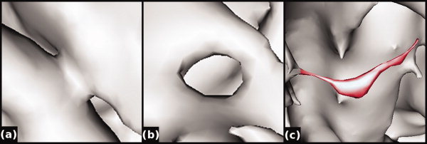
Common problems include topological defects and artifacts. Topological defects such as handles (a) and holes (b) prevent the surface from being homeomorphic with a sphere. By contrast, artifacts (c, highlighted in red) may permit a correct (spherical, genus‐zero) topology but nonetheless are anatomically incorrect and should ideally be eliminated during topology correction. [Color figure can be viewed in the online issue, which is available at wileyonlinelibrary.com.]

Topological defects can include handles (Fig. 1a) and holes (Fig. 1b) that prevent the surface from being homeomorphic with a sphere. In terms of topology, handles and holes are equivalent; however, the two may be differentiated in that during the topology correction process, handles should be cut but the holes should be filled. The number of defects in a given surface can be calculated using the Euler characteristic, where an Euler characteristic of 2 represents a surface that is homeomorphic with a sphere.1

Artifacts (Fig. 1c) are topologically correct sharp peaks (usually due to noise) that do not reflect true features of cortical anatomy. All of these errors need to be repaired before the surface can be inflated to a sphere. Because artifacts usually contain sharper edges than the rest of the cortical surface, they can be minimized via a smoothing process. However, accurately correcting topology defects is more difficult. Compared with previously proposed methods, we propose the use of regional spherical harmonic representations as a simple, straightforward method to correct these topological errors and geometrical artifacts.

Prior Approaches to Correct Topological Defects

There are two general approaches used to address topology defects. The first approach is to start with a surface with the desired topology and deform it to match the brain surface (a top‐down approach). The surface representation may either be discrete (such as a mesh) or continuous, and there are a number of approaches to deforming this initial surface. In this category are included active contours or deformable models. There is a wealth of literature on variations of this method applied to brain data; for a review, see [McInerney and Terzopoulos,1996; Montagnat et al.,2001]. Methods include fast marching algorithms [Bazin and Pham,2005a,b,2007a,b], level‐set methods [Bischoff and Kobbelt,2002,2003,2004; Xiao et al.,2003], minimization of an energy functional [Caselles et al.,1997; Dale et al.,1999; Karaçali and Davatzikos,2003; Kass et al.,1988; MacDonald et al.,2000], competitive forces [Delingette and Montagnat,2001; McInerney and Terzopoulos,2000], a system of constraints [Lachaud and Montanvert,1999], simplex meshes [Delingette,1999], homotopically deformable regions [Mangin et al.,1995], and diffeomorphic transformations of a digitized anatomical template [Christensen et al.,1994]. As the cortical surface is highly convoluted, a disadvantage of these approaches is that the fitting function is highly nonlinear and may require extensive computations. Furthermore, the resulting surface may not represent all of the deep sulci accurately [Fischl et al.,2001]. This is because typically high curvature regions are penalized during the evolution of the template, to make the extractions more robust to high frequency noise, and the resulting enforcement of regularity may restrain the evolving surface from correctly flowing into the deep sulci.

The second approach is to retrospectively correct the topology after the brain data have been segmented into WM and GM (a bottom‐up approach). These corrections may be achieved either in volume space or on a mesh surface generated using an algorithm such as marching cubes [Lorensen and Cline,1987]. A common volume‐based solution is to use graph‐based methods to detect topology defects and find the minimal modification required to correct the defect [Abrams et al.,2002,2004; Chen and Wagenknecht,2006; Han et al.,2002,2004; Jaume et al.,2005; Shattuck and Leahy,2001].

It is also possible to find the minimal modification directly on the surface [Guskov and Wood,2001]. By selecting just the minimal set, it is possible that the resulting correction is not identical to the changes that would be made by an experienced operator. Another possible solution is to filter the WM membership until the largest triangular mesh has a geometry homeomorphic to a sphere [Xu et al.,1999]. A drawback of this approach is that the filtering process essentially smoothes the WM and some anatomical information can be lost. In volume space, it is also possible to construct a skeleton to describe the shape of the volume, correct cycles within the skeleton, and then regrow the skeleton to form a topologically correct object [Zhou et al.,2007]. Finally, another volume‐based solution is based on region‐growing algorithms to correct the initial segmentation [Kriegeskorte and Goebel,2001; Ségonne et al.,2003].

Surface‐based methods often do not correct large handles appropriately but are appropriate for small topological defects. One method to circumvent this problem is to measure the defect size and then correct small defects in the surface and large defects in volume space [Wood et al.,2004]. The original MRI data may also inform retrospective topological corrections on the surface. The correction can then be carried out using purely surface‐based methods such as genetic algorithms [Ségonne et al.,2005], retessellation of the defect [Fischl et al.,2001], or nonseparating loops with opening operators [Segonne et al.,2007].

These methods vary widely in speed and accuracy. For deformable surfaces, the speed is usually related to the complexity of the fitting function. For retrospective correction methods, pure surface‐based methods tend to be slower, while it is possible to quickly repair topological defects using voxel‐based methods but possibly at a cost to accuracy.

Spherical Harmonics

We propose to use spherical harmonics for the first time to accurately correct topological defects directly on the surface. Spherical harmonics have been recently applied to brain surface meshes, usually in the realm of shape analysis. First applied to brain imaging in 1995, as a method to detect shape differences between closed objects [Brechbühler et al.,1995], and for representing the cortex and flows between surfaces [Thompson and Toga,1996], spherical harmonic analysis has been subsequently applied to quantify structural differences in subcortical structures [Gerig et al.,2001; Gutman et al.,2006; Kelemen et al.,1999; Shenton et al.,2002] and full cortical surfaces [Chung et al.,2006; Shen and Chung,2006].

Spherical harmonic analysis can be described as a Fourier transform on a sphere that decomposes the brain surface data into frequency components; the spherical harmonics are the eigenfunctions of the Laplacian operator on the sphere, and they are often used a basis to compute and estimate solutions to diffusion equations or flows in spherical coordinates, as they provide a complete orthogonal sequence of functions that can approximate any (square‐integrable) smooth function defined on the sphere (including, by analogy, the 3D spatial coordinates of a spherically parameterized surfaces, as they can be considered as functions on the sphere). The surface can also be reconstructed from the coefficients of the spherical harmonics. If spherical harmonics are used to approximate a reconstructed surface, the RMS error of the reconstructed surface decreases as the number of coefficients increases and can become arbitrary small (i.e., uniform approximation). Furthermore, the coefficients of the spherical harmonics may be weighted to achieve a smoothing effect [Chung et al.,2007].

A drawback to spherical harmonics is the computation time required to calculate the coefficients. However, a modification of the fast Fourier transform compatible with spherical coordinates dramatically decreases the computation time, as it is no longer necessary to directly calculate the coefficients [Healy et al.,1996; Kostelec et al.,2000].

In this article, we present a method to accurately correct topological defects and artifacts using spherical harmonics. Spherical harmonic functions retrospectively correct topological errors directly on the brain surface mesh. In brief, we resample a spherical mapping of the cortical surface mesh and calculate 3D spatial coordinates for each spherically sampled point based on its approximate location in the cortical surface mesh (Fig. 2b–d). The coordinates of location mapped on the regularly sampled sphere are forward transformed and then inversely transformed via spherical harmonics to reconstruct a cortical surface without topological defects (Fig. 2e,f). In a high‐frequency reconstruction, the topological defects are replaced with a spiked surface (high sharpness), which is repaired by replacing local patches with points from a low‐pass filtered reconstructed surface (Fig. 2g). The result is a more accurately reconstructed cortical surface free from topological defects and large geometrical artifacts (Fig. 2h).

Figure 2.

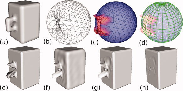
The full processing pipeline is illustrated using a simple shape with a handle. The original surface mesh (a) is mapped onto a sphere (b). The radii of points in the handle are modified so that they are no longer on the surface of the sphere (c). A regularly sampled grid (d, green) is then overlaid on top of this sphere to create uniform sampling in the parameter space. For each point in the regularly sampled grid (d, green), the intersecting triangle in the spherical mapping (d, blue) is found, and barycentric coordinates within this triangle are used to interpolate a spatial coordinate for this vertex lying on the original tessellated surface mesh. Points with modified radii are not favored during the search for nearest intersecting triangle. These regularly sampled points are forward‐ then reverse‐transformed using spherical harmonics. High‐frequency (e) and low‐pass filtered (f) reconstructed surfaces are derived from the spherical harmonic coefficients. In the regions containing the defect, vertices from the low‐pass filtered reconstruction are patched into the high‐bandwidth reconstruction (g). Finally, a T1 postcorrection step removes any remaining artifacts from the removal of the handle (h). [Color figure can be viewed in the online issue, which is available at wileyonlinelibrary.com.]

METHODS

Sample Data Sets

Three data sets were used to evaluate the validity of this approach: (a) an artificial structure containing topological defects and geometrical artifacts; (b) 12 MRI scans of the same brain, including the creation of a “gold standard” by averaging all 12 scans and manually correcting any remaining topology defects; and (c) scans of 10 healthy control subjects.

The topological phantom is essentially a cube that has three holes, two handles, and two “artifacts.” The 60‐mm³ phantom was made by simulating a 1‐mm³ T1 intensity image using routines available from the Statistical Parametric Mapping software package (http://www.fil.ion.ucl.ac.uk/spm/software/) and in‐house MatLab code and then constructing a surface mesh with ∼50 K triangles using a marching cubes algorithm. This surface mesh is then corrected using our method. Another simulated “gold standard” T1‐weighted image was also generated as an input for T1 image postcorrection. By comparing to the “gold standard” mesh surface created directly from the “gold standard” T1 intensity image, it is possible to quantitatively assess the validity of the spherical harmonic reconstruction.

The second approach was to create a “gold standard” brain by averaging 12 scans of the same subject. The averaging reduces Gaussian noise and the size and number of the topological defects but cannot remove all topological defects entirely. The remaining defects were extremely small and corrected manually using FreeSurfer [Fischl et al.,1999a]. The sample data set included 12 brain scans of the same subject performed on two different 1.5 T Siemens Vision scanners. Both scanners used 3D magnetization‐prepared gradient echo (MP‐RAGE) T1‐weighted sequences of 160 sagittal slices with voxel dimensions 1 mm × 1 mm × 1 mm and FOV = 256 mm. Scanner 1 parameters were TR/TE/FA = 11.4 ms/4.4 ms/15°, and Scanner 2 parameters were TR/TE/FA = 15 ms/5 ms/30°.

To verify that the spherical harmonic‐based correction approach was not optimized for a single brain, a third dataset of 10 healthy control subjects' brain scans was also included. For the 10 control subjects (4 females/6 males, mean age 35.3 years, ±11.3 SD), T1‐weighted images were obtained on a 1.5 T Philips Gyroscan ACSII. There were 256 sagittal slices per scan (1‐mm thickness, TR = 13 ms, TE = 5 ms, flip angle = 25°, field‐of‐view = 256 mm) with a matrix size of 256 × 256, resulting in an isotropic voxel size of 1 mm³. As no “gold standard” is available for comparison, the correction for these brains was validated by an expert who scored the validity of topological defect corrections in brains corrected either using our method or by FreeSurfer. The brains were randomly labeled such that the scorer was not informed about which correction method had been used to correct each brain.

For both datasets (12 scans of the same brain and 10 control subjects), each brain scan was processed using the default FreeSurfer processing pipeline to produce a WM surface representation for each hemisphere [Fischl et al.,1999a]. The surface used as input into our topological correction method was the xh.smoothwm surface before topological correction. The spherical mapping was additionally postprocessed using in‐house tools to improve the accuracy of the reparameterization [Yotter et al.,in‐press]. All individual surface meshes included a unique set of topological defects.

Software Implementation

The topology correction program was implemented in the C programming language. The code related to spherical harmonics was based on a publicly available spherical harmonic processing library [Kostelec and Rockmore,2004], and the final correction using the T1 intensity images used functions extracted from the BICPL software library (McConnell Brain Imaging Centre Programming Library, http://packages.bic.mni.mcgill.ca/). These functions are described in more detail below. All other code was developed in‐house.

Cut/Fill Operations and the Initial Spherical Mapping

A difficult problem to solve in brain surface mesh reconstruction is how to fill holes and cut handles. We propose a simple and fast new method compatible with the spherical harmonics approach to accomplish this.

To apply spherical harmonic analysis to the brain surface mesh, a spherical mapping of the uncorrected surface mesh must first be generated. This spherical mapping is not homeomorphic with a sphere, because it still contains defects. It is also beneficial to reduce area distortion in the spherical mapping, because this improves the reparameterization process, during which a coordinate of location based on the estimated cortical surface location is generated for each regularly spaced point in spherical coordinates [Yotter et al., in‐press]. Additionally, this spherical mapping may also be used to identify topological defects by locating self‐intersections in the spherical mapping [Fischl et al.,1999a]. Points associated with topological defects will be referred to as defect points in the following discussion.

During the reparameterization process (detailed below), regularly sampled spherical points are associated with a cortical location by finding the closest triangle in the spherical mapping and then using barycentric coordinates to interpolate its location on that triangular tile. By varying the radius of the defect points within the defects, it is possible to favor a subset of defect points, such that the outer points for holes (or the inner points for handles) are more likely to be chosen. These points are favored because they are closer to the surface of the reparameterized sphere, whereas the other points with nonunity radius are further away than they would have been had their radii not been modified. This affects the search for the closest point when mapping the original set of points to the reparameterized mesh.

First, the defects must be labeled for either cut or fill operations. This is accomplished by examining the intensity of the T1 image in the space central to the defect. If it is above a T1 intensity threshold (set to 99% of the average T1 threshold of nondefect points, a threshold which empirically performed best for correctly labeling holes and handles), then it is labeled as a hole to be filled; otherwise, it is a handle to be cut. For large defect areas with many topological errors (e.g., when the Euler characteristic is less than −10), this approach is not applicable. These large defect clusters invariably occur either at the ventricles or in the nonbrain area around the orbitofrontal cortex (the correction of which is shown in Fig. 11). For the ventricular defects, they are identified using their 3D position within the brain and marked as a hole to be filled; for the defects around the orbitofrontal cortex, they are always cut.

Figure 11.

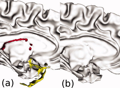
Large defect regions in the ventricular region are filled, whereas large defects in the nonbrain area around the orbitofrontal cortex are cut. (a) In the original uncorrected surface, the ventricular defect is marked in red and the defect around the orbitofrontal cortex is marked in yellow. (b) Spherical harmonics correction fills the ventricular defect and cuts the defect around the orbitofrontal cortex. [Color figure can be viewed in the online issue, which is available at wileyonlinelibrary.com.]

Once a defect has been labeled as a target for either a “cut” or a “fill” operation, the defect points are then bisected into two groups of points, based on how close they are to the cortical centroid, along the axis of the cortical defect.2 For defects marked for filling, the defect points closer to the cortical centroid are adjusted in the spherical mapping such that their radii are slightly smaller; for cutting, defect points farther from the cortical center have adjusted radii that are larger. Thus, during the reparameterization process, the closest polygon to the reparameterized point will more likely be the outer (for filling) or inner (for cutting) points within the defect region that contains overlapping triangles in the spherical mapping, as nonfavored points have been moved away from the surface of the reparameterized sphere. Figure 3 demonstrates this method for a hole.

Figure 3.

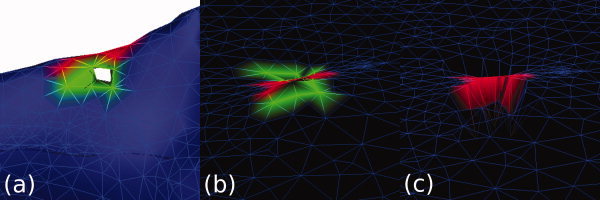
Defects are labeled as either holes for filling or handles for cutting before the surface is reparameterized. In this hole, the point set is first bisected (a). The original spherical mapping with the bisected points marked is shown in (b). Inner points (previously marked as green) are then modified on the spherical mapping to have a slightly smaller radius (c). When searching for the closest triangle during the reparameterization process, the outer triangles will be strongly favored. [Color figure can be viewed in the online issue, which is available at wileyonlinelibrary.com.]

Spherical Parameterization and Generation of Coordinates of Location

To analyze the harmonic content of a spherical surface, the spherical surface needs to have regularly sampled points with respect to θ and ϕ, where θ is the colatitude and ϕ is the azimuthal coordinate. As the original cortical surface does not generally map to a regularly sampled sphere, the first step in using spherical harmonics is to reparameterize the surface.

To do this, points are generated from equally sampled values of θ and ϕ for all members in the sets, such that there are 2B points per set, where B is the bandwidth. For each regularly sampled spherical point, the closest polygon on the cortical spherical mapping is found. Because of the change in the radius of defect points, these are slightly disfavored when searching for the closest polygon.

Within the closest polygon, a spatial location for the interpolated vertex in 3D is approximated using barycentric coordinates. The result is a regularly sampled spherical map in which every point is associated with a coordinate that gives its location on the original cortical surface (Fig. 2b–d).

Harmonic Analysis

The spherical harmonic series representation of a spherical mesh can be obtained using normalized spherical harmonics Y ${}_{\mathit{\text{m}}}^{\mathit{\text{l}}}$(θ,ϕ):

(1)

where l and m are integers with |m| ≤ l, and P ${}_{\mathit{\text{m}}}^{\mathit{\text{l}}}$ is the associated Legendre polynomial function defined by:

(2)

A square‐integrable function f(θ,ϕ) on the sphere can be expanded in the spherical harmonic basis such that:

(3)

where the coefficients f̂(l,m) are defined by the inner product f̂(l,m) = 〈f,Y ${}_{\mathit{\text{m}}}^{\mathit{\text{l}}}$〉, and the L ² norm of each basis function Y ${}_{\mathit{\text{m}}}^{\mathit{\text{l}}}$ is given by:

(4)

This system can be solved directly by finding the bases first, but a more efficient approach is to use a divide‐and‐conquer scheme as described in [Healy et al.,1996].

Using the calculated coefficients, two surfaces are reconstructed. The first surface is a high‐frequency surface that uses all coefficients as is (Fig. 2e). The second surface is a low‐bandwidth (smoothed) surface that is reconstructed from filtered coefficients using a 128‐order Butterworth low‐pass filter, thus excluding contributions from higher frequency coefficients (Fig. 2f). A Butterworth filter reduces ringing artifacts and results in a smoother reconstructed surface (see Fig. 4). To reconstruct the surfaces, the harmonic content is processed through an inverse Fourier transform to produce coordinates associated with each spherical point. These coordinates are used to reconstruct the cortical mesh without topological defects using an icosahedron as the base mesh.

Figure 4.

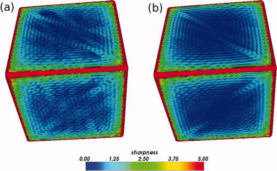
Using a Butterworth filter to filter the coefficients results in a smoother reconstructed surface. Both a boxcar filter (a) and a Butterworth filter (b) leave some ringing artifacts, but using a Butterworth filter reduces the magnitude of the ringing artifacts. The filtered reconstructions were obtained by initially calculating coefficients for l = 1,024, then filtering such that l _l = 64. These ringing artifacts can also be reduced by using a higher order spherical harmonic approximation. The sharpness of a mesh point is the maximum angle between the normals of nearest neighbor polygons, in degrees. [Color figure can be viewed in the online issue, which is available at wileyonlinelibrary.com.]

Patching of Reconstructed Cortical Meshes

After reconstruction via spherical harmonics, the resulting cortical mesh is homeomorphic to a sphere. However, two problems need to be addressed in the reconstructed surface. First, adjacent to regions formerly containing topological defects, the spherical harmonic‐based reconstructed surface generally replaces the defect with a spiked topology that does not correspond to actual brain anatomy. The spiked appearance is only present if the bandwidth is high enough to admit higher frequencies; if a lower bandwidth is used, the surface near former topological defects is smooth and well reconstructed, but anatomical detail is lost. Second, the reconstructed surface often contains self‐intersections that should be repaired; this problem is addressed in the next section.

To correct the first problem, these surfaces are combined such that the regions that exhibit spiked topology in the higher frequency (l = 1,024) surface are replaced with patches from the low‐pass filtered (l _l = 64) cortical reconstruction, but only in regions previously marked as defect areas (Fig. 2g). The lower limit was chosen such that the spiked regions were smooth but the surface retained the approximate shape of the original cortical surface, such that the union of the two surfaces does not result in large discontinuities (see Fig. 5).

Figure 5.

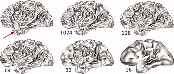
Some detail is lost as more coefficients are filtered. Filtering coefficients such that l _l = 32 or lower result in a surface that no longer resembles the original surface. The numbers shown are the lower value of l, and all surfaces were constructed such that l = 1,024 and then filtered with a Butterworth filter. An artifact (red arrow) is no longer visible in the surfaces reconstructed using spherical harmonics. [Color figure can be viewed in the online issue, which is available at wileyonlinelibrary.com.]

Regions with spiked topology are identified by calculating a sharpness value for each point. The sharpness is the maximum angle between the normals of nearest neighbor polygons. If the sharpness is above a threshold of t _s = 60°, and if this point is labeled as being within a region containing a topological defect, then this point and its set of nearest neighbors are replaced with the corresponding points in the low‐pass filtered cortical surface. This angular threshold was empirically determined to make sure that all brain surfaces were appropriately patched; however, as the patching only occurs within regions marked as areas formerly containing topological defects, lowering the threshold further had little effect on the final reconstructed surface.

Correcting Self‐Intersections

In all cases studied here, the reconstructed cortical surface contained self‐intersections, i.e., the cortical surface intersects itself. These self‐intersections generally occur in regions formerly containing topological defects and are found by testing for edge‐triangle intersections. Self‐intersections are undesirable, as it would mean that the same imaging data would be represented in at least two nonadjacent locations on the unfolded cortical surface. This problem should be addressed as part of the topological correction process. There are two approaches capable of resolving self‐intersections: further patching using the low‐pass filtered surface and localized smoothing.

As the low‐pass filtered reconstruction is smoother than the high‐frequency surface, it tends to contain fewer self‐intersections, as the lower frequency functions cannot easily generate a self‐intersection (as an extreme case, consider that low‐pass filtering such that l _l = 1 results in a sphere). By patching self‐intersection regions with the equivalent points from the low‐pass filtered surface, the number of self‐intersections can be greatly reduced, but usually not eliminated. This is the first step taken when repairing self‐intersections.

For remaining self‐intersections, the mesh is smoothed using a localized smoothing algorithm until the region no longer contains self‐intersections [Yotter et al.,in‐press). Figure 6 shows a typical example of self‐intersection smoothing. The localized smoothing algorithm was implemented such that it would not affect more than 0.1% of the total number of surface points. For details of this algorithm, see Appendix.

Figure 6.

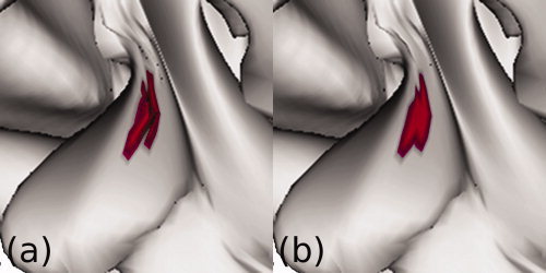
Self‐intersections are corrected via localized smoothing. A region containing self‐intersections (a) is smoothed until the cortical surface no longer intersects itself (b). The algorithm is implemented to affect as few points as possible. [Color figure can be viewed in the online issue, which is available at wileyonlinelibrary.com.]

T1 Image‐Based Postcorrection

It could be argued that the reparameterization, patching, and localized smoothing operations may result in a loss of fidelity in the spherical mapping. Furthermore, there may be some mislabeled defects that were cut/filled when the opposite operation would have been more appropriate. These issues can be counteracted by including a small amount of surface postprocessing based on the intensities of the associated T1‐weighted image (Fig. 2h). In our implementation, all points that were modified via patching or via self‐intersection repair are later adjusted using the original T1‐weighted intensity image and previously approximated T1 intensity threshold using the publicly available software package BICPL (http://packages.bic.mni.mcgill.ca/). The approach uses a surface deformation approach to correct the surface mesh based on the T1 intensity image [MacDonald et al.,1994]. This correction process uses only the T1 intensity image to reposition the surface mesh to locations in the T1 intensity image that are at a particular intensity threshold and tends to smooth the surface. By limiting this operation to only previously modified points and setting the maximum number of iterations to 40, the amount of smoothing of the surface is minimized.

Quantitative Analysis of Results

For the first two data sets (the phantom and 12 scans of the same brain), corrected surfaces were compared to the “gold standard” surface using the Hausdorff distance, the mean distance error, distance error histograms (for the second set only), and percentage of outlier reduction (defined below). The mean distance error d _e is the average minimum distance between a set of points X and a surface S, whereas the Hausdorff distance is the maximum value within the minimum distance set. The minimum distance function d(p,S) between a point p∈X and the surface S can be defined as:

(5)

where p′ is a point on the surface S. The mean distance error is then defined as follows

(6)

where N _p is the number of points in the set of points X.

The outlier reduction percent represents the fraction of points that remain above a distance error threshold set in the uncorrected brain surface, such that:

(7)

where N ^° _t and N _t are the number of points whose distance errors are above threshold in the original brain surface and the corrected surface, respectively, and N ^° _p and N _p are the total numbers of mesh points in the original brain surface and the corrected surface, respectively. The threshold is set to include the top 5% points with the largest distance errors in the uncorrected brain surface. A value of 100% indicates that all outliers have been removed, whereas a value of 0% indicates no improvement.

For the third dataset (10 scans of healthy control subjects), each topological defect was examined by an expert (R. D.) and given a score (+/0/− for accurate/partially accurate/inaccurate) based on the quality of the final surface. Here, a score of “0” or “partially accurate” means that the cut (or fill) was correct, but the corrected surface did not completely match the contours of the inner (or outer) surface in the original mesh.

RESULTS AND DISCUSSION

Topological Phantom

Although a topological phantom does not resemble a brain surface, topological defects in such a synthetic dataset should still be accurately repaired if the approach is fundamentally valid. Such datasets provide a way to assess accuracy when ground truth is known because it is specified analytically.

As shown in Figure 7, the topology is accurately corrected in a 60‐mm³ cubic phantom. Before T1 postcorrection, the topological correction algorithm shows good results filling holes and cutting handles. Furthermore, topologically correct but “inaccurate” geometrical artifacts are greatly reduced. The forward Hausdorff distance is 1.71 mm (due to the remaining geometrical artifacts (blue arrows) that originally deviated by 12 mm from the ideal surface), and the forward mean distance error is 4.7 μm.

Figure 7.

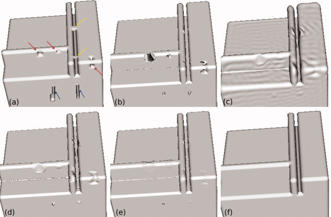
Topological correction using spherical harmonics relies on a union between a high‐frequency (l = 1,024) and low‐pass filtered (l _l = 64) surface. The original surface (a) contains three holes (red arrows), two handles (yellow arrows), and two geometrical artifacts (blue arrows). The high‐frequency reconstruction (b) replaces topological defects with sharp spikes but retains more detail than the low‐pass filtered surface (c). The union of the two surfaces (d) optimizes detail retention and topological error correction. T1 postcorrection smooths out the holes and handles (e), so that the corrected surface closely matches the ideal surface (f). [Color figure can be viewed in the online issue, which is available at wileyonlinelibrary.com.]

After T1 postcorrection, there are still some rounded edges in the phantom that deviate from the target surface. These highlight a key feature of the spherical harmonics approach, in that sharp edges are not preserved. As sharp edges do not exist in the folded surface of the brain, this might be considered to be an advantage of this approach, because it would correct these edges that must be due to noise. For surfaces with sharp edges, however, it would be important to choose a T1 postcorrection algorithm that does not contain a curvature limitation, as does the software package that we chose to use.

Twelve Scans of the Same Brain

The corrected surfaces were all homeomorphic to a sphere, verified by calculating the Euler characteristic. Quantitatively, our spherical harmonic method generated a corrected surface that has a lower distance error, an improved distance error histogram, and fewer outliers compared with the uncorrected surface, when both surfaces are compared with the ideal surface (Table I and Fig. 8). The corrected surfaces also contained fewer self‐intersections.

Table I.

Topological correction using spherical harmonics reduces the mean distance error and the proportion of the top 5% outliers in comparison with the averaged “gold standard” brain surface

Correction	Mean distance error (mm)		Hausdorff distance (mm)		Outlier reduction (top 5%)	Total self‐intersections
	Forward	Reverse	Forward	Reverse
None	0.749 (±0.007)	0.509 (±0.008)	10.949 (±0.022)	4.332 (±0.032)	—	13
FreeSurfer	0.641 (±0.007)	0.563 (±0.007)	7.910 (±0.056)	5.270 (±0.041)	65.4%	21
SPH	0.537 (±0.007)	0.539 (±0.008)	6.855 (±0.044)	5.922 (±0.034)	85.1%	3

Generally, the forward Hausdorff distance and mean distance error metrics measure how well the reconstructed surface matches the “gold standard” mesh; the reverse Hausdorff distance and mean distance error indicate how much information in the “gold standard” mesh was retained in the reconstruction.

Figure 8.

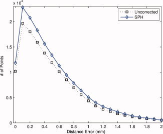
The forward distance error histogram is improved for surfaces corrected using the spherical harmonic method. The histograms are an average compiled for 24 hemispheres. Compared with the uncorrected surfaces, there are more points with low or zero distance error for the spherical harmonic corrected surfaces. [Color figure can be viewed in the online issue, which is available at wileyonlinelibrary.com.]

Visual inspection reveals that most corrections were closer to the “gold standard” averaged brain surface compared with the original uncorrected surface. Typical corrections are shown in Figure 9. By mapping the distance error across the surface of a single brain, the distance error located in nondefect regions closely matched the distance error in the uncorrected surface (see Fig. 10). In previously published algorithms, large defects were sometimes problematic for the correction processes. However, our approach accurately corrects large defects. Figure 11 shows typical corrections in the ventricular region and the nonbrain area around the orbitofrontal cortex.

Figure 9.

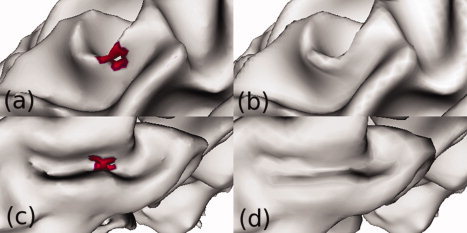
A typical correction of topological defects by spherical harmonics is shown. Holes (a) are filled (b), and handles (c) are cut (d). [Color figure can be viewed in the online issue, which is available at wileyonlinelibrary.com.]

Figure 10.

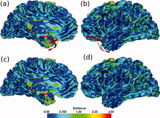
Away from topological defects, surface information remains unchanged. The uncorrected surfaces (a and b) are almost identical to the spherical harmonics corrected surfaces (c and d), except in regions near topological defects. The distance in mm is the error between these surfaces and the “gold standard” averaged surface. [Color figure can be viewed in the online issue, which is available at wileyonlinelibrary.com.]

Because the averaged “gold standard” brain may be smoothed during the averaging process, it could be argued that the smoothing due to spherical harmonics is the primary cause of the reduced distance error metrics. However, by measuring the distance error from the original uncorrected surface, it is clear that the spherical harmonics reconstruction is highly representative of the original uncorrected surface, despite the fact that the surface has been reparameterized (Table II). This is further shown by the low mean distance errors. As expected, the reverse Hausdorff distance is large because of the removal of large defects and artifacts. Changes in these areas are also responsible for an increase in the reverse mean distance error.

Table II.

The mean distance errors for surfaces corrected using topological correction are small when compared with the original uncorrected surface

Correction	Mean distance error (mm)		Hausdorff distance (mm)
	Forward	Reverse	Forward	Reverse
FreeSurfer	0.227 (±0.006)	0.408 (±0.005)	4.186 (±0.037)	10.592 (±0.075)
SPH	0.011 (±0.000)	0.309 (±0.002)	3.031 (±0.018)	11.025 (±0.037)

However, the reverse Hausdorff distance is large because of the removal of defects.

The full topology correction process using spherical harmonics (including identification of defects, smoothing, patching, and so on) requires ∼6–8 min on a 2.4‐GHz iMac for a mesh that contains 150,000 vertices. This excludes the initial spherical mapping generation and T1 postcorrection; the latter step requires ∼8 min of additional processing time. The resulting mesh contains approximately the same number of vertices. As a basis of comparison, the topology correction process in the standard FreeSurfer pipeline takes approximately an hour; however, as no source code is available, it is unknown whether other operations besides topological correction are performed during this processing step.

Ten Scans of Healthy Controls

Ten additional brain surfaces were processed, and each defect correction was rated by an expert. The expert was provided with two corrections per hemisphere that had been randomly grouped with the goal of obtaining an unbiased correction score; however, when questioned afterward, it was clear to the expert which brain surface was corrected using which method, due primarily to the corrections performed for the ventricular areas. Spherical harmonic correction accurately repaired topological defects in 93% of the cases (score of + or 0), of which 9% were only partially correct. For the remaining 7% (score of −), the errors arose from incorrect labeling for fill/cut operations or incorrect bisecting of the defect points due to an unusual geometry of the defect. As a point of comparison, the standard FreeSurfer pipeline accurately repaired 94% of the defects, of which 3% were only partially correct.

CONCLUSION

Topology correction using spherical harmonics successfully removes topology defects and reduces geometrical artifacts. The approach is also valid for large defects that contain multiple holes and handles (Euler characteristic less than −10). It accurately corrects most of the topological defects, and considering that this is a new approach, it is expected that, with future refinements, the correction accuracy may increase in the future.

One source of error is in misclassification of holes and handles, resulting in holes being cut and handles being filled. The approach presented here relies on the T1‐weighted image intensity in the center of the defect to differentiate between the two cases. A more complicated algorithm that takes into account the location of the defect on the surface of the brain, the T1‐weighted intensity image surrounding the defect, and even curvature values may improve classification accuracy. One important tradeoff is the computation time required for a more complicated approach, which may offer limited improvement in accuracy.

Another source of improvement would be in the T1‐based postcorrection process. In this implementation, we chose to use a publicly available software package that does not account for the method with which the surfaces were originally corrected. A global T1 postcorrection algorithm that is compatible with spherical harmonics (for example, by making assumptions about the initial smoothness of the reconstructed surface or by examining the original uncorrected surface) could increase the accuracy of this correction step without a noticeable sacrifice in computation speed. Furthermore, the T1‐based postcorrection was only applied to the topological defects; it is expected that a T1‐based postcorrection applied globally to the entire surface would further increase the accuracy of the reconstructed surface.

The topological errors (especially the large defect in the area around the orbitofrontal cortex) arose initially from incorrect segmentation of tissue types. The accuracy of tissue segmentation could be improved by using tissue registration [Ashburner and Friston,2005]. However, depending on the surface construction algorithm, the improved segmentation accuracy may not help to reduce the size and number of handles across gyri, because the spaces between gyri would still be relatively narrow.

In conclusion, we found that topological correction using spherical harmonics offers a fast, accurate method to correct topological defects in cortical surfaces used in brain mapping. We verified this both qualitatively and quantitatively. As the approach is fairly straightforward, it lends itself to inclusion in a full processing pipeline for surface data. The topology of surfaces generated using this method are more accurate than the original uncorrected surface, are homeomorphic with a sphere, and are suitable for intersubject analysis.

AREA SMOOTHING ALGORITHM

Self‐intersections are resolved by smoothing the mesh locally. First, the self‐intersection region is labeled. Edge points are then “anchored” such that the points within the edge points are the only ones that are smoothed. Given an inner point p, each triangle adjacent to the point is assigned a weight that is used to adjust the position of the point. The center of each triangle t _j containing point p is found using the formula:

(8)

where r and s are the other two points in the triangle. The weight w _j of triangle t _j is set such that:

(9)

where A _p is the total area of all triangles containing point p. The position of point p can then be updated as follows:

(10)

where N is the number of triangles containing point p. The inner points are smoothed for five iterations; if the self‐intersection is not resolved, the edge points are moved by one neighboring point such that the smoothed area inside the edge point set increases. If the number of smoothed points reaches ∼0.1% of the total mesh points (threshold of 100 points), the self‐intersections are remapped such that the edges are tight, i.e., they directly neighbor the self‐intersection. The remapping limits the number of points affected by smoothing.

REFERENCES

- Abrams L, Fishkind DE, Priebe CE ( 2002): A proof of the spherical homeomorphism conjecture for surfaces. IEEE Trans Med Imaging 21: 1564–1566. [DOI] [PubMed] [Google Scholar]
- Abrams L, Fishkind DE, Priebe CE ( 2004): The generalized spherical homeomorphism theorem for digital images. IEEE Trans Med Imaging 23: 655–657. [DOI] [PubMed] [Google Scholar]
- Ashburner J, Friston KJ ( 2005): Unified segmentation. Neuroimage 26: 839–851. [DOI] [PubMed] [Google Scholar]
- Ballmaier M, Kumar A, Thompson PM, Narr KL, Lavretsky H, Estanol L, DeLuca H, Toga AW ( 2004): Localizing gray matter deficits in late‐onset depression using computational cortical pattern matching methods. Am J Psychiatry 161: 2091–2099. [DOI] [PubMed] [Google Scholar]
- Bazin P‐L, Pham DL ( 2005a): Topology correction using fast marching methods and its application to brain segmentation In: Duncan J, Gerig G, editors. MICCAI. Palm Springs, CA: Springer; pp 484–491. [DOI] [PubMed] [Google Scholar]
- Bazin P‐L, Pham DL ( 2005b): Topology preserving tissue classification with fast marching and topology templates In: Christensen GE, Sonka M, editors. Information Processing in Medical Imaging. Glenwood Springs, CO: Springer; pp 234–245. [DOI] [PubMed] [Google Scholar]
- Bazin P‐L, Pham DL ( 2007a): Topology correction of segmented medical images using a fast marching algorithm. Comput Methods Programs Biomed 88: 182–190. [DOI] [PMC free article] [PubMed] [Google Scholar]
- Bazin P‐L, Pham DL ( 2007b): Topology‐preserving tissue classification of magnetic resonance brain images. IEEE Trans Med Imaging 26: 487–496. [DOI] [PubMed] [Google Scholar]
- Bearden CE, Erp TGMv, Thompson PM, Toga AW, Cannon TD ( 2007a): Cortical mapping of genotype‐phenotype relationships in schizophrenia. Hum Brain Mapp 28: 519–532. [DOI] [PMC free article] [PubMed] [Google Scholar]
- Bearden CE, van Erp TGM, Dutton RA, Tran H, Zimmermann L, Sun D, Geaga JA, Simon TJ, Glahn DC, Cannon TD, Emanuel BS, Toga AW, Thompson PM ( 2007b): Mapping cortical thickness in children with 22q11.2 deletions. Cereb Cortex 17: 1889–1898. [DOI] [PMC free article] [PubMed] [Google Scholar]
- Bischoff S, Kobbelt LP ( 2002): Isosurface reconstruction with topology control In: Coquillart S, Shum H‐Y, Hu S‐M, editors. Proceedings of the 10th Pacific Conference on Computer Graphics and Applications. Beijing: IEEE Computer Society; pp 246–255. [Google Scholar]
- Bischoff S, Kobbelt L ( 2003): Sub‐voxel topology control for level‐set surfaces. Comput Graph Forum 22: 273–280. [Google Scholar]
- Bischoff S, Kobbelt L ( 2004): Topologically correct extraction of the cortical surface of a brain using level‐set methods. In: Tolxdorff T, Braun J, Handels H, Horsch A, Meinzer H‐P, editors. Proceedings of BVM. Berlin: Springer‐Verlag; pp 50–54. [Google Scholar]
- Brechbühler C, Gerig G, Kübler O ( 1995): Parametrization of closed surfaces for 3‐D shape description. Comput Vis Image Understand 61: 154–170. [Google Scholar]
- Caselles V, Kimmel R, Sapiro G ( 1997): Geodesic active contours. Int J Comput Vis 22: 61–79. [Google Scholar]
- Chen L, Wagenknecht G ( 2006): Automated topology correction for human brain segmentation In: Larsen R, Nielsen M, Sporring J, editors. MICCAI. Copenhagen, Denmark: Springer; pp 316–323. [DOI] [PubMed] [Google Scholar]
- Christensen GE, Rabbitt RD, Miller MI ( 1994): 3D brain mapping using a deformable neuroanatomy. Phys Med Biol 39: 609–618. [DOI] [PubMed] [Google Scholar]
- Chung M, Shen L, Dalton K, Davidson R ( 2006): Multi‐scale voxel‐based morphometry via weighted spherical harmonic representation In: Yang G‐Z, Jiang T, Shen D, Gu L, Yang J, editors. Medical Imaging and Augmented Reality. Shanghai: Springer; pp 36–43. [Google Scholar]
- Chung MK, Dalton KM, Li S, Evans AC, Davidson RJ ( 2007): Weighted Fourier series representation and its application to quantifying the amount of gray matter. IEEE Trans Med Imaging 26: 566–581. [DOI] [PubMed] [Google Scholar]
- Dale AM, Fischl B, Sereno MI ( 1999): Cortical surface‐based analysis. I. Segmentation and surface reconstruction. Neuroimage 9: 179–194. [DOI] [PubMed] [Google Scholar]
- Delingette H ( 1999): General object reconstruction based on simplex meshes. Int J Comput Vis 32: 111–146. [Google Scholar]
- Delingette H, Montagnat J ( 2001): Shape and topology constraints on parametric active contours. Comput Vis Image Understand 83: 140–171. [Google Scholar]
- Desai R, Liebenthal E, Possing ET, Waldron E, Binder JR ( 2005): Volumetric vs. surface‐based alignment for localization of auditory cortex activation. Neuroimage 26: 1019–1029. [DOI] [PubMed] [Google Scholar]
- Fischl B, Sereno MI, Dale AM ( 1999a): Cortical surface‐based analysis. II. Inflation, flattening, and a surface‐based coordinate system. Neuroimage 9: 195–207. [DOI] [PubMed] [Google Scholar]
- Fischl B, Sereno MI, Tootell RBH, Dale AM ( 1999b): High‐resolution intersubject averaging and a coordinate system for the cortical surface. Hum Brain Mapp 8: 272–284. [DOI] [PMC free article] [PubMed] [Google Scholar]
- Fischl B, Liu A, Dale AM ( 2001): Automated manifold surgery: Constructing geometrically accurate and topologically correct models of the human cerebral cortex. IEEE Trans Med Imaging 20: 70–80. [DOI] [PubMed] [Google Scholar]
- Formisano E, Esposito F, Di Salle F, Goebel R ( 2004): Cortex‐based independent component analysis of fMRI time series. Magn Reson Imaging 22: 1493–1504. [DOI] [PubMed] [Google Scholar]
- Gaser C, Luders E, Thompson PM, Lee AD, Dutton RA, Geaga JA, Hayashi KM, Bellugi U, Galaburda AM, Korenberg JR, Mills DL, Toga AW, Reiss AL ( 2006): Increased local gyrification mapped in Williams syndrome. Neuroimage 33: 46–54. [DOI] [PubMed] [Google Scholar]
- Gerig G, Styner M, Jones D, Weinberger D, Lieberman J ( 2001): Shape analysis of brain ventricles using SPHARM In: Mathematical Methods in Biomedical Image Analysis (MMBIA). Kauai, HI: IEEE; pp 171–178. [Google Scholar]
- Guskov I, Wood ZJ ( 2001): Topological noise removal In: Proceedings of Graphics Interface. Ottawa, Ontario, Canada: Canadian Information Processing Society; pp 19–26. [Google Scholar]
- Gutman B, Wang Y, Lui LM, Chan TF, Thompson PM ( 2006): Hippocampal surface analysis using spherical harmonic function applied to surface conformal mapping In: International Conference on Pattern Recognition (ICPR). Hong Kong, China: IEEE Computer Society; pp 964–967. [Google Scholar]
- Han X, Xu C, Braga‐Neto U, Prince JL ( 2002): Topology correction in brain cortex segmentation using a multiscale, graph‐based algorithm. IEEE Trans Med Imaging 21: 109–121. [DOI] [PubMed] [Google Scholar]
- Han X, Pham DL, Tosun D, Rettmann ME, Xu C, Prince JL ( 2004): 3RUISE: Cortical reconstruction using implicit surface evolution. Neuroimage 23: 997–1012. [DOI] [PubMed] [Google Scholar]
- Healy DM, Rockmore DN, Moore SSB ( 1996): FFTs for the 2‐Sphere—Improvements and Variations. Technical Report PCS‐TR96–292, Dartmouth College.
- Hinds OP, Rajendran N, Polimeni JR, Augustinack JC, Wiggins G, Wald LL, Diana Rosas H, Potthast A, Schwartz EL, Fischl B ( 2008): Accurate prediction of V1 location from cortical folds in a surface coordinate system. Neuroimage 39: 1585–1599. [DOI] [PMC free article] [PubMed] [Google Scholar]
- Hurdal MK, Stephenson K ( 2009): Discrete conformal methods for cortical brain flattening. Neuroimage 45: S86–S98. [DOI] [PubMed] [Google Scholar]
- Jaume S, Rondao P, Macq B ( 2005): Open topology: A toolkit for brain isosurface correction In: Duncan J, Gerig G, editors. MICCAI. Palm Springs, CA: Springer. [Google Scholar]
- Karaçali B, Davatzikos C ( 2003): Topology preservation and regularity in estimated deformation fields In: Taylor C, Noble JA, editors. Information Processing in Medical Imaging. Ambleside, UK: Springer; pp 426–437. [PubMed] [Google Scholar]
- Kass M, Witkin A, Terzopoulos D ( 1988): Snakes: Active contour models. Int J Comput Vis 1: 321–331. [Google Scholar]
- Kelemen A, Szekely G, Gerig G ( 1999): Elastic model‐based segmentation of 3‐D neuroradiological data sets. IEEE Trans Med Imaging 18: 828–839. [DOI] [PubMed] [Google Scholar]
- Kostelec PJ, Rockmore DN ( 2004): S2kit: A Lite Version of SpharmonicKit. Hanover, NH: Department of Mathematics, Dartmouth College. [Google Scholar]
- Kostelec PJ, Maslen DK, Dennis M, Healy J, Rockmore DN ( 2000): Computational harmonic analysis for tensor fields on the two‐sphere. J Comput Phys 162: 514–535. [Google Scholar]
- Kriegeskorte N, Goebel R ( 2001): An efficient algorithm for topologically correct segmentation of the cortical sheet in anatomical MR volumes. Neuroimage 14: 329–346. [DOI] [PubMed] [Google Scholar]
- Lachaud J‐O, Montanvert A ( 1999): Deformable meshes with automated topology changes for coarse‐to‐fine three‐dimensional surface extraction. Med Image Anal 3: 187–207. [DOI] [PubMed] [Google Scholar]
- Lerch JP, Pruessner JC, Zijdenbos A, Hampel H, Teipel SJ, Evans AC ( 2005): Focal decline of cortical thickness in Alzheimer's disease identified by computational neuroanatomy. Cereb Cortex 15: 995–1001. [DOI] [PubMed] [Google Scholar]
- Lin JJ, Salamon N, Lee AD, Dutton RA, Geaga JA, Hayashi KM, Luders E, Toga AW, Engel J Jr, Thompson PM ( 2007): Reduced neocortical thickness and complexity mapped in mesial temporal lobe epilepsy with hippocampal sclerosis. Cereb Cortex 17: 2007–2018. [DOI] [PubMed] [Google Scholar]
- Lorensen WE, Cline HE ( 1987): Marching cubes: A high resolution 3D surface construction algorithm In: Stone MC, editor. SIGGRAPH: 14th Annual Conference on Computer Graphics and Interactive Techniques. Anaheim, CA: ACM; pp 163–169. [Google Scholar]
- Lui L, Wang Y, Chan T, Thompson P ( 2006): A landmark‐based brain conformal parameterization with automatic landmark tracking technique In: Larsen R, Nielsen M, Sporring J, editors. Medical Image Computing and Computer‐Assisted Intervention—MICCAI 2006. Copenhagen, Denmark: Springer‐Verlag, New York; pp 308–315. [DOI] [PubMed] [Google Scholar]
- Lui LM, Wang Y, Chan TF, Thompson P ( 2007): Landmark constrained genus zero surface conformal mapping and its application to brain mapping research. Appl Numer Math 57: 847–858. [Google Scholar]
- MacDonald D, Avis D, Evans AC ( 1994): Multiple surface identification and matching in magnetic resonance images In: Robb RA, editor. Visualization in Biomedical Computing 1994. Rochester, MN: SPIE; pp 160–169. [Google Scholar]
- MacDonald D, Kabani N, Avis D, Evans AC ( 2000): Automated 3‐D extraction of inner and outer surfaces of cerebral cortex from MRI. Neuroimage 12: 340–356. [DOI] [PubMed] [Google Scholar]
- Mangin J‐F, Frouin V, Bloch I, Régis J, López‐Krahe J ( 1995): From 3D magnetic resonance images to structural representations of the cortex topography using topology preserving deformations. J Math Imaging Vis 5: 297–318. [Google Scholar]
- McInerney T, Terzopoulos D ( 1996): Deformable models in medical image analysis: A survey. Med Image Anal 1: 91–108. [DOI] [PubMed] [Google Scholar]
- McInerney T, Terzopoulos D ( 2000): T‐snakes: Topology adaptive snakes. Med Image Anal 4: 73–91. [DOI] [PubMed] [Google Scholar]
- Montagnat J, Delingette H, Ayache N ( 2001): A review of deformable surfaces: Topology, geometry and deformation. Image Vis Comput 19: 1023–1040. [Google Scholar]
- Narr KL, Bilder RM, Toga AW, Woods RP, Rex DE, Szeszko PR, Robinson D, Sevy S, Gunduz‐Bruce H, Wang Y‐P, DeLuca H, Thompson PM ( 2005): Mapping cortical thickness and gray matter concentration in first episode schizophrenia. Cereb Cortex 15: 708–719. [DOI] [PubMed] [Google Scholar]
- Qiu A, Younes L, Wang L, Ratnanather JT, Gillepsie SK, Kaplan G, Csernansky J, Miller MI ( 2007): Combining anatomical manifold information via diffeomorphic metric mappings for studying cortical thinning of the cingulate gyrus in schizophrenia. Neuroimage 37: 821–833. [DOI] [PMC free article] [PubMed] [Google Scholar]
- Ségonne F, Grimson E, Fischl B ( 2003): Topological correction of subcortical segmentation In: Ellis RE, Peters TM, editors. MICCAI. Montreal, Canada: Springer; pp 695–702. [Google Scholar]
- Ségonne F, Grimson E, Fischl B ( 2005): A genetic algorithm for the topology correction of cortical surfaces In: Christensen GE, Sonka M, editors. Proceedings of Information Processing in Medical Imaging. Glenwood Springs, CO: Springer; pp 393–405. [DOI] [PubMed] [Google Scholar]
- Segonne F, Pacheco J, Fischl B ( 2007): Geometrically accurate topology‐correction of cortical surfaces using nonseparating loops. IEEE Trans Med Imaging 26: 518–529. [DOI] [PubMed] [Google Scholar]
- Shattuck DW, Leahy RM ( 2001): Automated graph‐based analysis and correction of cortical volume topology. IEEE Trans Med Imaging 20: 1167–1177. [DOI] [PubMed] [Google Scholar]
- Shen L, Chung MK ( 2006): Large‐scale modeling of parametric surfaces using spherical harmonics In: 3DPVT. Chapel Hill, NC: IEEE Computer Society; pp 294–301. [Google Scholar]
- Shenton ME, Gerig G, McCarley RW, SzÈkely Gb, Kikinis R ( 2002): Amygdala‐hippocampal shape differences in schizophrenia: The application of 3D shape models to volumetric MR data. Psychiatry Res 115: 15–35. [DOI] [PMC free article] [PubMed] [Google Scholar]
- Thompson PM, Toga AW ( 1996): A surface‐based technique for warping three‐dimensional images of the brain. IEEE Trans Med Imaging 15: 402–417. [DOI] [PubMed] [Google Scholar]
- Thompson PM, Hayashi KM, Sowell ER, Gogtay N, Giedd JN, Rapoport JL, de Zubicaray GI, Janke AL, Rose SE, Semple J, Doddrell DM, Wang Y, van Erp TGM, Cannon TD, Toga AW ( 2004): Mapping cortical change in Alzheimer's disease, brain development, and schizophrenia. Neuroimage 23: S2–S18. [DOI] [PubMed] [Google Scholar]
- Thompson PM, Lee AD, Dutton RA, Geaga JA, Hayashi KM, Eckert MA, Bellugi U, Galaburda AM, Korenberg JR, Mills DL, Toga AW, Reiss AL ( 2005): Abnormal cortical complexity and thickness profiles mapped in Williams syndrome. J Neurosci 25: 4146–4158. [DOI] [PMC free article] [PubMed] [Google Scholar]
- Thompson PM, Bartzokis G, Hayashi KM, Klunder AD, Lu PH, Edwards N, Hong MS, Yu M, Geaga JA, Toga AW, Charles C, Perkins DO, McEvoy J, Hamer RM, Tohen M, Tollefson GD, Lieberman JA, Group THS ( 2009): Time‐lapse mapping of cortical changes in schizophrenia with different treatments. Cereb Cortex 19: 1107–1123. [DOI] [PMC free article] [PubMed] [Google Scholar]
- Tosun D, Reiss AL, Lee AD, Dutton RA, Hayashi KM, Bellugi U, Galaburda AM, Korenberg JR, Mills DL, Toga AW, Thompson PM ( 2006): Use of 3‐D cortical morphometry for mapping increased cortical gyrification and complexity in Williams syndrome In: IEEE International Symposium on Biomedical Imaging (ISBI2006), Arlington, VA, USA. [Google Scholar]
- Van Essen DC ( 2004): Surface‐based approaches to spatial localization and registration in primate cerebral cortex. Neuroimage 23: S97–S107. [DOI] [PubMed] [Google Scholar]
- Van Essen DC ( 2005): A population‐average, landmark‐ and surface‐based (PALS) atlas of human cerebral cortex. Neuroimage 28: 635–662. [DOI] [PubMed] [Google Scholar]
- Van Essen DC, Drury HA ( 1997): Structural and functional analyses of human cerebral cortex using a surface‐based atlas. J Neurosci 17: 7079–7102. [DOI] [PMC free article] [PubMed] [Google Scholar]
- Van Essen DC, Maunsell JHR ( 1980): Two‐dimensional maps of the cerebral cortex. J Comp Neurol 191: 255–281. [DOI] [PubMed] [Google Scholar]
- Wang Y, Chiang M‐C, Thompson PM ( 2005): Automated surface matching using mutual information applied to Riemann surface structures In: Duncan J, Gerig G, editors. Medical Image Computing and Computer‐Assisted Intervention—MICCAI 2005. Palm Springs, CA: Springer Berlin/Heidelberg; pp 666–674. [DOI] [PubMed] [Google Scholar]
- Wang Y, Gu X, Chan TF, Thompson PM, Yau S‐T ( 2008): Conformal slit mapping and its applications to brain surface parameterization In: Metaxas DN, Axel L, Fichtinger G, Szekely G, editors. International Conference on Medical Image Computing and Computer Assisted Intervention—MICCAI 2008. New York City, NY: Springer Berlin/Heidelberg; pp 585–593. [DOI] [PubMed] [Google Scholar]
- Wang Y, Dai W, Gu X, Chan TF, Yau S‐T, Toga AW, Thompson PM ( 2009): Teichmüller shape space theory and its application to brain morphometry In: Yang G‐Z, Hawkes DJ, Rueckert D, Noble JA, Taylor CJ, editors. Medical Image Computing and Computer Assisted Intervention (MICCAI2009). London, UK: Springer Berlin/Heidelberg; pp 131–140. [DOI] [PubMed] [Google Scholar]
- Wang Y, Zhang J, Gutman B, Chan TF, Becker JT, Aizenstein HJ, Lopez OL, Tamburo RJ, Toga AW, Thompson PM ( 2010): Multivariate tensor‐based morphometry on surfaces: Application to mapping ventricular abnormalities in HIV/AIDS. Neuroimage 49: 2141–2157. [DOI] [PMC free article] [PubMed] [Google Scholar]
- Wood Z, Hoppe H, Desbrun M, Schröder P ( 2004): Removing excess topology from isosurfaces. ACM Trans Graph 23: 190–208. [Google Scholar]
- Xiao H, Chenyang X, Prince JL ( 2003): A topology preserving level set method for geometric deformable models. IEEE Trans Pattern Anal Mach Intell 25: 755–768. [Google Scholar]
- Xu C, Pham DL, Rettmann ME, Yu DN, Prince JL ( 1999): Reconstruction of the human cerebral cortex from magnetic resonance images. IEEE Trans Med Imaging 18: 467–480. [DOI] [PubMed] [Google Scholar]
- Yotter RA, Thompson PM, Gaser C: Algorithms to improve the re‐parameterization of spherical mappings of brain surface meshes. 2000. J Neuroimag, in‐press. [DOI] [PubMed] [Google Scholar]
- Zhou Q‐Y, Ju T, Hu S‐M ( 2007): Topology repair of solid models using skeletons. IEEE Trans Visual Comput Graph 13: 675–685. [DOI] [PubMed] [Google Scholar]