

Abstract
It is a challenge for current signal analysis approaches to identify the electrophysiological brain signatures of continuous natural speech that the subject is listening to. To relate magnetoencephalographic (MEG) brain responses to the physical properties of such speech stimuli, we applied canonical correlation analysis (CCA) and a Bayesian mixture of CCA analyzers to extract MEG features related to the speech envelope. Seven healthy adults listened to news for an hour while their brain signals were recorded with whole‐scalp MEG. We found shared signal time series (canonical variates) between the MEG signals and speech envelopes at 0.5–12 Hz. By splitting the test signals into equal‐length fragments from 2 to 65 s (corresponding to 703 down to 21 pieces per the total speech stimulus) we obtained better than chance‐level identification for speech fragments longer than 2–3 s, not used in the model training. The applied analysis approach thus allowed identification of segments of natural speech by means of partial reconstruction of the continuous speech envelope (i.e., the intensity variations of the speech sounds) from MEG responses, provided means to empirically assess the time scales obtainable in speech decoding with the canonical variates, and it demonstrated accurate identification of the heard speech fragments from the MEG data. Hum Brain Mapp, 2013. © 2012 Wiley Periodicals, Inc.
Keywords: auditory perception, decoding, encoding, machine learning, magnetoencephalography, signal processing, speech
INTRODUCTION
As a fundamental prerequisite for speech perception and comprehension, our brains have a remarkable ability to follow the rapidly changing sound sequence of natural speech. The speech sounds naturally leave traces to the listener's brain activity, but still it has remained highly challenging to identify perceptual correlates of natural continuous speech in e.g. magnetoencephalographic (MEG) and electroencephalographic (EEG) signals. The main reason has been the lack of suitable data analysis methods for nonaveraged ongoing MEG/EEG signals. Here we introduce a novel signal‐analysis approach that attempts to extract MEG responses elicited by continuous speech and even enables us to identify, on the basis of the MEG signature, the related speech fragment.
Previously, single words or phrases have been associated with MEG/EEG responses on the basis of pattern classification [Guimaraes et al., 2007; Luo and Poeppel, 2007; Suppes et al., 1997, 1998, 1999]; either single‐trial or averaged response waveforms were matched to prototype waveforms of each class of words or phrases, created by averaging over tens or hundreds of trials in 3–48 classes. The most successful single‐trial MEG classification so far was 60.1% (with cross‐validation) for nine auditorily presented words in a set of 900 trials; however, the result was from a single subject only [Guimaraes et al., 2007].
In natural speech, acoustical features such as pitch, loudness, and rhythm vary all the time, and hence both the speech signal and brain activity signal have a complex dynamic nature with a fairly unpredictable systemic behavior. Consequently, classification based on prototype responses to words or sentences may not be an ideal approach, because the number of possible brain signatures can grow enormously large for free‐running speech. In this article, we take an alternative approach by modeling the relationship between the time series of speech signal and the related brain responses as stimulus‐related components and features. As an advantage, the features could then be predicted for any given time instant, even for words and expressions not heard during the model training.
MEG and EEG responses are known to be influenced by the intensity variation of the speech signal (i.e., the speech envelope). For example, when the sentence “The young boy left home” was presented 1000 times, the mean peak correlation between the averaged EEG response and the speech envelope reached 0.37 [Abrams et al., 2008]. Interestingly, the correlation between EEG response waveform and the stimulus envelope was related to the comprehension level of speech presented in different tempos [Abrams et al., 2008, 2009; Ahissar et al., 2001; Nourski et al., 2009]. The onsets and offsets of phones, syllables and words in the speech envelope provide information about the rhythmicity of speech. The speech envelope also contains prosodic cues [Rosen, 1992]. According to behavioral studies, envelope frequencies below 16 Hz have a crucial role in speech communication and understanding [Drullmanet al., 1994a, b; Houtgast and Steeneken, 1985; Shannon et al., 1995; Smith et al., 2002; Steeneken and Houtgast, 1980].
In this article, we focus on MEG features that contain information about the temporal structure of heard speech within time scales of a few seconds. Our subjects were listening to a news broadcast for 1 h. We searched for MEG features that would correlate with the time series of the speech envelope. We further studied how short an MEG epoch can be and still have a discriminative value about the speech stimulus. For this purpose, we split the test signals into fragments and, while increasing the fragment size gradually in consequent runs from 2 s on, we attempted to identify the speech fragment that the subject had been listening to at a given time. The key methodology here builds on the canonical correlation analysis (CCA) and on a new Bayesian mixture of CCA's developed specifically for this purpose.
MATERIALS AND METHODS
Subjects
Seven native Finnish‐speaking healthy subjects (4 females, 3 males, ages 20–41, 2 left‐handed) participated in the study. All subjects reported normal hearing. The MEG recordings had a prior approval by the ethics committee of Helsinki and Uusimaa Hospital district, and all participants gave their written informed consent for the study.
Recordings
Subjects listened to a collection of short news articles read by a native female Finnish speaker. The articles considered two general topics [earlier used by Hirsimäki et al., 2006]. The total duration of the news was 58 min. The subjects were sitting in a magnetically shielded room with the head leaning against the inner vault of the MEG helmet. During a short break in the middle of the session, the subjects were allowed to leave the shielded room. A nonmagnetic open‐field audio speaker (Panphonics, Tampere, Finland), over 2.5 m away from the subject, produced a comfortable loudness for the speech sounds. A map of Europe (72 by 55 cm) was fixed about 1.5 m in front of the subject for free viewing during the recordings. The subjects were instructed to listen attentively to the news reports. For a couple of subjects, a brief alerting sound was given (about one to three times) during the recording if signs of decreased vigilance were observed in the continuous video monitoring or eye movement and eye blink recording. For two subjects, an additional break was given to prevent drowsiness.
MEG was recorded with a 306‐channel neuromagnetometer (Elekta Neuromag, Elekta Oy, Helsinki, Finland). The recording passband was 0.1–200 Hz, and the signals were sampled at 600 Hz. Vertical electro‐oculogram (EOG) was recorded but was not utilized in later signal processing. Four head‐position‐indicator coils were attached to the head surface for continuous monitoring of the head position.
Data Preprocessing
Magnetic interference arising from sources outside the brain was suppressed by temporal signal space separation (tSSS; Taulu and Simola, 2006) implemented in the MaxFilter software (Elekta Oy, Helsinki, Finland). The default parameters of the program were used: 4‐s data buffer; 0.98 subspace correlation limit; inside expansion order 8, outside expansion order 3; 80 inside and 15 outside harmonic terms. Continuous head position compensation (200 ms windows in 10 ms steps minimum) and the conversion of the data into the standard head position were also accomplished with the Maxfilter software.
The speech envelope was computed by rectifying the acoustic signal (sampled at 16 kHz) and down‐sampling it with an antialiasing filter to 600 Hz. Although the down‐sampled signal had basically the same sampling rate as the MEG signal, a minor difference in the internal clocks of the MEG device and the stimulus computer kept the signals slightly unsynchronized. The ratio (1.0002) between the sampling intervals of the audio file and the MEG file was used to interpolate the audio envelope to exactly match the MEG sampling rate. Cross‐correlation was additionally used to adjust the true audio envelope and the reference audio signal (rectified offline) recorded on one channel of the MEG data‐acquisition system. The audio envelope was transformed by log10(1+x) [Aiken and Picton, 2008]. Both the envelope and the MEG data were normalized by z‐scoring; they were resampled to 25, 50, and 100 Hz sets to enable extracting different frequency ranges with the CCA models (see the next section).
The analyzed data comprised three sets. A 32‐min recording covering one general news topic was split into two sets, one for training (training set, ∼20 min) and one for evaluation of the statistical significance of the CCA findings (validation set, ∼10 min). The rest of the data, comprising another news topic, were used as an independent test set (test set, 26 min).
Obviously, the stimulus–response relationship governing brain reactivity during audible speech is disrupted during long silences. Therefore, to limit violations of the stationarity assumption of the classical CCA modeling, the data sets were manipulated by shortening the silence periods down to 25 sampling points (e.g., with 25 Hz sampling frequency the maximum allowed silence duration was 1 s). Most of the removed periods were pauses between two news articles. Instead, short breaks related to, e.g., respiration and text punctuation remained unaffected. This procedure removed altogether 5 min of silent periods from the training set, 2 min from the validation set, and 3 min from the test set.
Another reason for removing of the silent periods originates from the identification procedure (described later) based on splitting the test signal into fragments. Each fragment is assumed to hold a unique stimulus waveform, and for fragments of silence this assumption would not hold.
Classical CCA
In our application, the classical CCA [Hotelling, 1936] was used for modeling the stimulus–response relationship. With CCA it was possible (i) to find the MEG channels that respond to the stimulus, (ii) to estimate the response delay, (iii) to specify the mutually correlating signal components from the envelope and MEG signals (i.e., to find the shared signal components), and (iv) to estimate the correlation coefficient for these components.
From the data‐analysis standpoint, the speech envelope and the recorded MEG are two paired multidimensional data sets, say X and Y, and the task is to find statistical dependencies between the feature vectors x ∈ X and y ∈ Y in a data‐driven way. Basically, CCA finds such weighting (canonical basis vectors
 and
and
 ) for the two data vectors x and y that the resulting random variables (called canonical variates) u and v are maximally correlated. Here,
 and
and
 . In other words, CCA maximizes the function
| (1) |
where ρ is the correlation between the first pair of canonical variables. The other pairs can be found in a similar fashion but with the constraint that all the pairs are uncorrelated. With noisy data, the rank of the data sets X and Y is typically larger than the number of significantly correlating canonical variates. Therefore, CCA provides a means for dimensionality reduction. In other words, the canonical variates provide a compact representation of the common variation in the two data sets, discarding much of the noise present in either feature vector alone. It is, however, worth noticing that the CCA model assumes a linear stimulus–response relationship over the whole experiment and that the observations are independent. The former assumption will later be relaxed in the Bayesian mixture of CCA models. Deviation from the latter assumption due to autocorrelation of the observations can lead to overestimation of canonical correlations, but as demonstrated later with control data analysis, the deviations in our data do not cause notable effects.
We analyzed the signals in time windows. The feature vectors were composed of the l successive signal values in time, e.g., x 1 = {x 1, x 2,…,x l}T, x 2 = {x 2, x 3,…,x l+1}T. The vector length, and thus all the canonical basis vectors, was 25 points. To let the CCA models be sensitive to different frequency ranges, three sampling frequencies (25, 50, and 100 Hz) were used in the experiments. Therefore, l = 25 corresponds to windows of 1 s, 500 ms, and 250 ms, respectively. Larger windows were not used because then the feature vectors would have contained much redundancy and could have caused problems with numerical solutions. As the feature vectors consisted of data points in specified time windows, the canonical basis vectors can be interpreted as kernels of finite‐impulse‐response (FIR) filters and CCA as a tool to find specific correlated waveforms (or passbands) in the two signals. Such kernels, as studied with Fourier analysis, have an intuitive frequency‐band interpretation. Figure 1 gives an example of the basis vectors.
Figure 1.
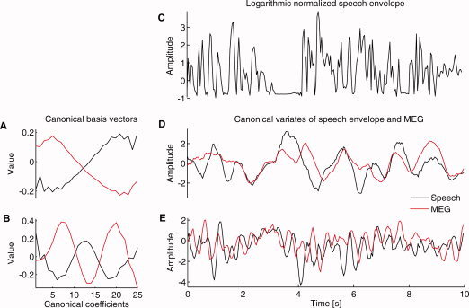
An example of CCA analysis. Data come from a single gradiometer over the right temporal cortex of Subject #2 who showed the largest correlations in the group. A,B: Two sets of basis vectors are shown. The red lines indicate the MEG and the black lines the speech‐envelope counterparts. The upper pair (A) represents basis vectors sensitive to 0.5 Hz fluctuations and the bottom pair (B) to 2.5 Hz fluctuations. The basis vectors may differ for the two data sources and need not be in the same phase. On the top of the right column (C), a 10‐s piece of the (logarithmic) speech envelope training data is shown. Below (D and E), for the same piece of data, the canonical variables corresponding to the basis vectors on the left are presented. With all training data of this subject, canonical correlation r = 0.37 for the 0.5 Hz fluctuation, and r = 0.26 for the 2.5 Hz fluctuation.
The delay of MEG responses, with respect to the eliciting sound, was estimated by delaying the MEG signal by 0–500 ms, training the CCA model at each delay, and finally by evaluating the correlation between the first pair of canonical variates. This procedure is a multivariate extension of cross‐correlation analysis. We tested for the statistical significance of the correlations using the delay of the maximum correlation. To prevent the circular inference [Kriegeskorte et al., 2009], the delay was chosen based on correlation on the training data, but for significance testing the model was used to predict the canonical variate time series for the validation data (which was separate from the final test data used later for identification). The validation set was divided into 30‐s nonoverlapping segments (corresponding to 17 or more segments, depending on the subject and the sampling rate). For each segment, Pearson correlation was calculated between all (N = 25) pairs of canonical variates. A two‐tailed Wilcoxon signed rank test was used to assess whether the correlation values of the predicted data deviate from zero with the Bonferroni‐corrected significance level P < 0.05/N. The procedure was repeated for each individual, for the three sampling frequencies (25, 50, and 100 Hz), and for each of the 306 channels separately. This procedure simultaneously revealed the statistically significant shared signal components between the datasets, the informative MEG channels, and the physiological delays.
Bayesian Mixture of CCA Models
While the basic principle of CCA extends to prediction tasks, the simple model of Eq. (1) is too limited to accurately capture the relationship between the stimuli and the brain signals. For instance, the model assumes the two data sources to be jointly stationary over the whole experiment. However, according to our data this assumption may not hold even within the training set, since pauses in the speech envelope lead to different dynamics than the ongoing speech and, strictly speaking, the simple preprocessing steps, such as removing long pauses, are not sufficient to make the signal stationary.
In this section we present a novel model for more accurate modeling of the stimulus–response relationship and for better‐geared predictions of future data. The model improves on the classical CCA in three respects: (i) it replaces the stationarity assumption by local stationarity of short time segments, (ii) it is more robust for deviations from the Gaussian noise assumption implicit in classical CCA, and (iii) it is less likely to find spurious correlations between the data sources (that is, nonexistent stimulus–response relationships).
The model builds on the Bayesian interpretation of CCA [Klami and Kaski, 2007; Wang, 2007], formulating the task of extracting correlations between the speech envelope and the brain response as a generative latent‐variable model. Given the latent‐variable formulation, the above improvements can be included in the model by extending the generative description. First, the stationarity assumption is relaxed by building a mixture of CCA models. Roughly speaking, the mixture is based on the assumption that different CCA models are responsible for explaining different clusters in the data space. The clusters here refer to the temporal data partitions that show different kinds of stimulus–response relationships between the speech envelope and MEG data. The partitioning of the data into the clusters, training of the different CCA models for each individual cluster, and optimization of the various model parameters are done automatically and in a data‐driven way. For a more extensive description of mixture models, see McLachlan and Peel [2000].
We applied the Bayesian mixture of CCA models for analyzing the MEG channels found to have the strongest MEG‐speech‐relationships with the classical CCA model, using the same channel‐wise response delays and the same feature‐vector compositions as in classical CCA. As the 25‐Hz sampling rate yielded the largest correlations, we applied it for the further analysis.
The following description of the Bayesian mixture of CCA models is based on the earlier conference publication of Viinikanoja et al. [2010]. The Matlab implementation is available from http://research.ics.tkk.fi/mi/software/vbcca/.
The standard CCA formulation implicitly assumes each set of variables to follow a multivariate normal distribution. However, this assumption does not hold in practice, especially for the speech envelope. We thus replace the assumption of Gaussian noise in the generative model by assuming that the noise follows Student's t‐distribution. The t‐distribution is bell‐shaped like the normal distribution but has heavier tails; hence, the outlier data values have a smaller effect on the model, making it more robust to signal artifacts and non‐Gaussianity of signals in general.
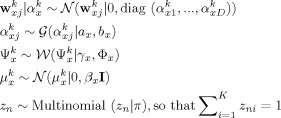
The complete model, coined Bayesian mixture of CCAs (Fig. 2), is defined by the conditional probability densities
 |
 |
Figure 2.
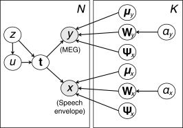
Graphical representation of the Bayesian mixture of CCA models as a plate diagram. The shaded nodes x and y represent the observed speech and MEG signal windows, respectively, whereas the non‐shaded nodes indicate the latent variables (z, u, t) and model parameters (the rest). For the purpose of this work, the most important variable is the latent variable t that captures the equivalent of canonical variates, a low‐dimensional representation of the stimulus–response relationship. The remaining variables are described in the main text. The left‐most plate indicates replication over the N samples and the right‐most plate over the K clusters or mixture components of the model.
Here
 denotes the normal distribution with mean b and precision c evaluated at a,
  is the Wishart distribution, and
  is the gamma distribution. The subscript k denotes the cluster indices and D denotes the latent space dimensionality. The random vectors x and y correspond to the speech envelope and the MEG signal in temporal windows, the latent variable t encodes the analogs of canonical variates, u implements robustness, z indicates the cluster membership, and the columns of the projections matrices W
x and W
y define the shapes of the dependent waveforms.
is the gamma distribution. The subscript k denotes the cluster indices and D denotes the latent space dimensionality. The random vectors x and y correspond to the speech envelope and the MEG signal in temporal windows, the latent variable t encodes the analogs of canonical variates, u implements robustness, z indicates the cluster membership, and the columns of the projections matrices W
x and W
y define the shapes of the dependent waveforms.
To avoid the need to manually specify the number of correlating components for each of the K clusters, we adopt the Automatic Relevance Determination (ARD) prior for the projection matrix row vectors
 through the Gamma prior
 for the precisions. With a relatively noninformative prior for α via a
x = b
x = 0.1, the precisions for unnecessary components are driven to infinity during inference, forcing the components to converge towards zero vectors with no influence on the model. This procedure improves the specificity of the model as extracting spurious correlations is discouraged; yet high correlations are not suppressed by the ARD prior. For the rest of the hyperparameters, we choose fixed values corresponding to broad priors (γx = dim(x)+1, βx = 1) and hence we let the data determine the model parameters. Finally, ϕx is set to the diagonal matrix c
I where the magnitude of the constant c is deduced from the empirical covariance of the data X, and π is learned by using a point estimate. The priors related to the other data source y are identical and are not repeated here.
for the precisions. With a relatively noninformative prior for α via a
x = b
x = 0.1, the precisions for unnecessary components are driven to infinity during inference, forcing the components to converge towards zero vectors with no influence on the model. This procedure improves the specificity of the model as extracting spurious correlations is discouraged; yet high correlations are not suppressed by the ARD prior. For the rest of the hyperparameters, we choose fixed values corresponding to broad priors (γx = dim(x)+1, βx = 1) and hence we let the data determine the model parameters. Finally, ϕx is set to the diagonal matrix c
I where the magnitude of the constant c is deduced from the empirical covariance of the data X, and π is learned by using a point estimate. The priors related to the other data source y are identical and are not repeated here.
Following the Bayesian modeling principles, the predictions are averaged over the posterior distribution of the model parameters given the data. However, the posterior distribution cannot be inferred analytically and needs to be approximated. We adopt the variational approximation [Jordan et al., 1999] and approximate the posterior distribution by the following factorized distribution:
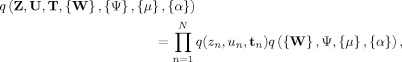 |
where the term containing the parameters is further factorized as
The individual terms q of the approximation are learned by minimizing the Kullback‐Leibler divergence between the approximation and the true distribution,
Given the above factorization, the minimization task leads to analytically tractable update rules for each of the distributions q and these update rules are combined into a single EM‐style algorithm.
Speech Fragment Identification
Beyond the correlation and the descriptions of the correlating signal components, we were interested in studying whether the speech envelope could be predicted from MEG signals in the time‐domain. Specifically, we wanted to inspect to what extent it is possible to predict from the MEG signals features of speech envelope at a particular instant. With CCA‐type models we can first learn the correlating subspace that contains the features common to the two paired data sets (i.e., the canonical variates with the classical CCA, latent variable t with the Bayesian mixture of CCA models), and then use the trained model to predict the feature values in this subspace at certain instances for a completely new data set. Successful predictions of this sort would indicate stable and consistent brain responses, since the prediction can be accurate only if the stimulus–response relationship is similar over the whole recording. Furthermore, the model needs to correctly capture the essential relationships.
We were interested in finding out whether the specific fragments of the news stimuli could be identified based on the predicted latent‐variable waveforms (for more extensive background and the motivation of this approach, see Discussion). In more specific terms, the identification task was to infer the underlying stimulus from an observed MEG epoch given the 23‐min test set of MEG and the speech envelope data, both split into fragments of equal lengths (in no particular order). We repeated this analysis using different fragment lengths, ranging from 2 s to 65 s, corresponding to 703 down to 21 pieces per the total speech stimulus. Note that the canonical variate time series within the fragments were 1 s shorter due to the feature‐vector composition. For each individual fragment of the MEG variates, the best matching speech‐envelope counterpart was selected by means of correlation, as will be described below.
For comparison, the identification was carried out both with the classical CCA and with the Bayesian mixture of CCA models. In the latter case, both the training and the validation data sets were used for training. The number of clusters was originally set to four and the dimension of the latent signal t was set to equal the number of significant CCA components. The automatic relevance determination, incorporated in the model, was allowed to fine‐tune the dimensionality separately for each cluster (i.e., for each CCA model in the mixture). The latent‐variable t time series were predicted separately for MEG and for the logarithmic speech envelope signals. The prediction resulted in two multidimensional data sets representing the time series in each dimension of t predicted for each cluster. We call these data sets canonical variates of speech and canonical variates of MEG. In addition to t, also the dominating cluster was predicted at each time instant on the basis of speech envelopes that better discriminate sustained speech from pauses than does the MEG signal.
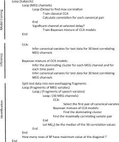
The pairs of canonical variate time series were predicted for the testing data within each fragment. Pearson correlation was calculated between all the i–j pairs, representing the fragment with the canonical variates of MEG and the fragment with the canonical variates of speech, respectively. Correlation was calculated for each signal dimension and of these the largest was selected as the representative value of the i–j pair correlation. Given the fragment i of canonical variates for one channel of MEG, and fragment j of the speech variates, the Pearson correlation was calculated between the corresponding time series in the matrices and the largest value was selected for further processing. We did not calculate the correlation between all corresponding time series, but only between those that corresponded to the dominating cluster (>50% of the fragment length), i.e. to sustained speech. The procedure was repeated for 30 MEG channels (except for Subject 7 who had only 24 significant channels) as ranked by the correlations of classical CCA. We used the median of these 30 values to find the maximally correlating ij pair. If this value was largest for i = j, the identification was considered as correct. We note that the way of combining the multichannel data was an ad hoc solution, chosen as the first choice tried and not optimized to prevent the circular inference [Kriegeskorte et al., 2009]. Figure 3 illustrates this procedure. With the classical CCA, the procedure was basically equivalent but simpler, because the stimulus–response relationship was modeled with only one CCA model. Table I outlines the main analysis steps as pseudo‐code for both modeling approaches.
Figure 3.
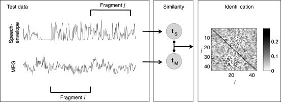
Schematic illustration of the main identification steps: (i) Canonical variate time series for test data were predicted both for speech envelope data (t S) and for MEG data (t M) and divided into fragments indexed by j for speech and i for MEG. (ii) Correlation was calculated between t M in the fragment i and t S in fragment j. The procedure was repeated for the 30 significant MEG channels. If the median correlation value over the channels was the largest when i = j, the identification was considered correct. The matrix in the figure represents the median correlation values as gray‐scale between fragments i and j when the number of fragments was ∼40. This number was used as a parameter in the identification procedure.
Table 1.
Algorithm summarizing the main analysis phases
|
The Binomial test was used to assess, for each subject, whether the number of correct identifications is statistically significantly (P < 0.05) higher than would be expected given a series of random identifications (n trials equals the number of fragments; the probability of a random correct identification is 1/n). As the test was repeated for individual subjects, the Bonferroni correction was applied. The significance was assessed separately for each fragment size.
RESULTS
MEG Responses to Continuous Speech
Figure 1 illustrates the stimulus–response relationship between speech sounds and MEG signals, modeled separately for the pairs of each individual MEG channel and the speech envelope by the classical CCA; this analysis resulted in estimates of channel‐wise response delays, correlating waveforms (canonical variates) and their correlation coefficients.
Figure 4 summarizes the results. Statistically significant correlations (P < 0.05, correlation > 0.1) with the stimulus envelope were found in lateral planar gradiometer and magnetometer channels. No systematic hemispheric dominance was observed. The canonical basis vectors often represented narrow frequency bands throughout the 0.5–12 Hz range (Figs. 1 and 4). However, the low frequencies below 3 Hz were dominating: they involved more channels than the higher frequencies and gained the maximum correlations > 0.3. The correlation maximum in the MEG signal typically occurred with about 150‐ms delay (Fig. 5) with respect to the stimulus envelope.
Figure 4.
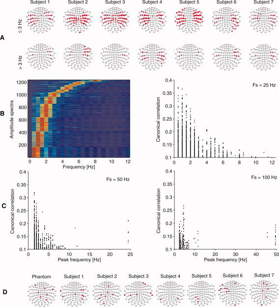
MEG responses to speech, from the classical CCA. A: Topographic maps of 306 MEG sensors (nose upwards). The top panel displays channels responding to AM frequencies ≤ 3 Hz and the bottom panel to > 3 Hz. Statistically significant canonical correlations exceeding 0.1 are marked with red dots. B: Left: The frequency response of the canonical basis vectors of MEG in color scale (arbitrary units), pooled over the seven subjects and sorted by the peak frequency. Right: Pooled correlations as a function of the peak basis vector frequency. In (A) and (B) the results are from data resampled to 25 Hz (sampling frequency Fs; see text for details). C: Corresponding correlations with the two other sampling frequencies. D: MEG channels passing the significance limit in the control data analysis. The maximum correlation of any of these channels was 0.055.
Figure 5.
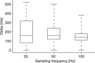
The estimated delays of MEG responses for the three sampling frequencies used, pooled over the channels with significant canonical correlations of the seven subjects. The box‐plot represents the 25th, 50th, and 75th percentiles and the whiskers the extent of data.
MEG channels with statistically significant correlations were selected for further analysis with the Bayesian mixture of CCA models. Importantly, if the stimulus–response relationship was not consistent throughout the recording, at this stage separate CCA models were automatically trained for different conditions. As a result, the time series were modeled with mixtures of four CCA models. As a parameter of the algorithm, this number of clusters was considered sufficient, because typically only one cluster was dominating for 80–83% of the time (minimum 43%) in the training data (Fig. 6). (In the testing data, the dominating cluster was also predicted with the result that one single cluster covered the data 94–100% of time). The rest of the models were related to shorter periods, such as pauses in speech. All these learned CCA models were used in the next stages of the analysis.
Figure 6.
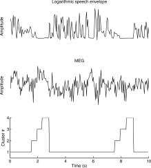
An example of the dominating cluster estimation. Different clusters here represent different stimulus–response relationships between the speech envelope and one MEG channel. Note that in the figure, one time instant t in the cluster data represents window t − 0.5…t + 0.5 s in the speech and MEG data. Apparently, cluster #1 represents the epochs of sustained speech; the other clusters represent pauses or transition periods from sustained speech to pauses and vice versa.
Control Data Analysis
To rule out the possibility that the findings would be due to some artifacts—such as induced magnetic fields from the stimulus system, faults in the recording set‐up, or spurious effects of data processing—we did a recording with a MEG phantom [Elekta Oy, Helsinki, Finland; e.g. Taulu et al., 2004] using the same stimuli and analysis as with our human subjects (training set and test set). Additionally, we reanalyzed the human recordings by reversing the speech envelopes in offline analysis. In these settings, the statistically significant correlations between speech‐envelope and MEG signals were maximally 0.055, which is low compared with the maximum correlations of 0.37 in the original setting with classical CCA. Moreover, the corresponding MEG channels were topographically scattered without any systematic clustering to certain brain region, in contrast to the actual human recordings (Fig. 4D). The result was further confirmed by training the Bayesian mixture of CCA models with the phantom data. Predictions for the training data showed maximal correlation of 0.032 (with the dominating cluster), compared with 0.279 in the human subjects. Thus, the results with the control data were not consistent with the physiological findings as was expected given that we used a nonmagnetic speaker more than 2.5 m away from the subject. To be on the safe side, only those MEG channels that showed correlations above 0.1 with the classical CCA were selected for the identification.
Identification of the Speech Fragments
Our objective was to infer the correct stimulus–response pair (i.e., MEG and speech envelope counterparts) given the 23‐min test data (not used for model training) split into fragments of equal lengths (in no particular order). The fragment durations ranged from 2 to 65 s. Thus, the identification performance was assessed with data sets divided to 703 down to 21 pieces, respectively.
The identification performance was consistent in six out of seven subjects (Fig. 7). The data of Subject 7 showed considerably worse performance (the outlier in Fig. 7A), and the subject was excluded from the following statistical analyses. The 90% (median) correct identification was exceeded with 40‐s fragments, and the identification reached 100% (median) with 55‐s fragments (with the Bayesian mixture of CCA models). For all fragment lengths, the results with at least five correct identifications are statistically significant (P < 0.05; Bonferroni corrected) according to the subject‐specific Binomial test. For all fragments longer than 5 s, the accuracy of all subjects differs statistically significantly from chance, clearly demonstrating successful identification. Even for the shortest 2‐, 3‐, and 5‐s fragments, the accuracy was significant for some subjects (5/6, 6/6, and 6/6 for the classical CCA model and 1/6, 5/6, and 5/6 for the Bayesian mixture of CCAs, respectively for the three fragment lengths).
Figure 7.
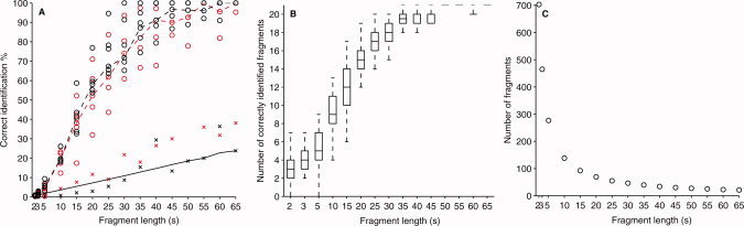
A: The performance of the speech‐fragment identification for each of the seven subjects using the Bayesian mixture of CCA models (red) and with the classical CCA (black). Points with “x”‐signs are outliers that originate from the Subject 7 data. The dashed line marks the median performance, and the solid line represents the minimum level for statistically significant identification (P < 0.05). B: Subject 1 data was reassessed by repeating the identification procedure 50 times with randomly chosen set of 21 separate fragments. The boxplots represents the 25th, 50th, and 75th percentile and the whiskers mark the extent of the correctly identified fragments. C: The testing data of 23 min were divided into consecutive time frames of equal length that determine the maximum number of fragments.
For comparison, the same identification procedure was carried out with control data (reversed speech signal for all seven subjects, and empty‐room measurement) from those MEG channels that passed the significance tests (without the requirement for the canonical correlations to exceed 0.1). Only the classic CCA modeling was used. No statistically significant identification accuracies were obtained for any of these control scenarios, irrespective of the fragment length.
To confirm that the identification performance depended on the fragment size and was not a spurious function of the number of fragments, we re‐assessed the data of Subject 1 with the Bayesian mixture of CCA models by limiting the number of fragments to 21 with all fragment sizes. The identification was repeated 50 times for each fragment size, each time with a randomly chosen set of 21 separate fragments (Fig. 7B). The results were similar to those in Figure 7A, which supports the length of the fragment, rather than the number of the fragments, as the decisive parameter affecting the identification performance.
DISCUSSION
MEG Responses to Continuous Speech
We searched for MEG signal features that correlate with the envelope of the heard speech. Both signals shared components, suggesting that MEG signals of the auditory cortex reflect the envelope of speech sounds. The shared components (i.e., the canonical variates) showed fluctuations at 0.5–12 Hz, which are important for speech comprehension [Drullman et al., 1994a, b; Houtgast and Steeneken, 1985; Shannon et al., 1995; Steeneken and Houtgast, 1980].
Luo and Poeppel [2007] recently suggested that speech affects the phase of the listener's MEG theta band (4–8 Hz) oscillations, corresponding to the syllabic rate of speech, and Aiken and Picton [2008] also suggested that the speech envelope is reflected in EEG mainly between 2 and 7 Hz, with a peak at 4 Hz. Our current results suggest that the correspondence with the speech envelope may extend considerably beyond the theta band and syllabic rate, to fluctuations below 3 Hz likely corresponding to words and sentences, as well as short pauses between them. The observed delays of MEG responses (∼150 ms) are in agreement with previous data [Aiken and Picton, 2008]. The prominence of the slowest frequencies in our results is concordant with Bourguignon et al., [2011] who, studying the coupling between listener's MEG and the f0 of the voice recorded with an accelerometer attached to the reader's throat, found the strongest coherence at about 0.5 Hz.
Identification of the Speech Fragments
We were interested in determining the time scales at which natural speech can be identified from the listener's brain activity. More specifically, we wanted to find out whether the heard speech can be identified from the listener's MEG signals at word, sentence or passage level. Thus, CCA and the Bayesian mixture of CCA models were used for predicting the canonical variates for separate testing data. We assessed the time scales of the predicted time series empirically by searching for the smallest fragment size valid for speech identification.
As the characteristics of freely running speech vary all the time, even short speech fragments differ from each other. For reliable identification, also the corresponding MEG signals need to have unique signatures, and ultimately the minimum fragment length sufficient for identification will depend on the similarity of the MEG and speech envelope waveforms. Because of the high variability of unaveraged MEG signals, at least 2–3‐s epochs were needed to guarantee distinctive stimulus‐related signal variation that resulted in above chance‐level identification of the fragment, corresponding to the time scale of sentences or a few words in speech. This happened even though the correlation values were modestly below 0.3. Instead, fragments of tens of seconds of duration were identified reliably; the accuracy exceeded 90% with the fragments of 40 s or more. As the largest correlations of the shared components occurred in frequencies below 3 Hz, it is likely that the identification also was influenced mostly by these low frequencies. Thus, in the assessment of the temporal accuracy of MEG responses, determining the valid time scales for the speech identification offered a complementary and intuitive aspect that was not directly obtainable from the correlation values.
Modeling the Stimulus–Response Relationship
Pattern classification methods have an important role as the first step in revealing perceptual correlates from the multivariate brain signals [e.g., Cox and Savoy, 2003; Dehaene et al., 1998; Haxby et al., 2001]. A more recent development, especially with fMRI recordings, has considered encoding models (or forward models) that describe stimulus‐related activity in small volume elements, and decoding models (inverse models) that infer characteristics of the stimulus on the basis of the brain responses [Thirion et al., 2006; Friston et al., 2008; Naselaris et al., 2011]. For example, based on the knowledge of visual cortex function, Kay et al., [2008] were able to build up an encoding model by first decomposing natural images to Gabor wavelet pyramids that could be utilized to predict the response in individual voxels by linear regression models. The predicted responses were compared with real recordings to identify which one picture in the set a person had seen. In their following work [Naselaris et al., 2009], natural pictures could be partially reconstructed from the brain activity using the decoding models. Stimulus reconstruction has been adopted also e.g. by Miyawaki et al. [2008] and Thirion et al. [2006].
Note that since the identification used by Kay and collaborators was based on the correlation between predicted and measured brain responses, the most decisive factor was the goodness of the encoding model. In identification, each sample is assigned to a distinct label and the used data are not necessarily included in the training set. In classification, to the contrary, the brain responses are assigned to one of few known categories, each explicitly presented in the training data. For more detailed comparison between identification and classification, see Kay et al. [2008].
In our work, CCA‐type models were adopted to describe the stimulus–response relationship and to predict instantaneous values of the canonical‐variate time series. CCA can be seen as a data‐driven approach to find shared signal subspaces where the two multivariate data sets correlate maximally. In the context of encoding and decoding, CCA appears as a special case because of its bidirectional nature. As the intermediate shared signal components (canonical variates) were predicted from both the MEG and speech signal directions, part of CCA behaves as an encoding model, and another part as a decoding model. Thus, the shared components can have different interpretations depending on the direction of prediction; they reflect the brain responses to speech stimuli, but equally well they can be considered as a partial reconstruction of the heard speech signal. It is important in practice that the decoding and encoding parts of the trained models can be used independently for prediction on new data.
The ability of the models to find shared signal components is generally affected both by the validity of the linearity and other modeling assumptions, and by the consistency and the temporal precision of the brain responses in following the speech envelope. Therefore, positive findings here imply that the modeling assumptions should hold and the brain responses should stay relatively stable at least to the degree where finding the linearly related and statistically significant shared signal components becomes possible.
In our CCA implementation, the feature vectors consisted of data points in sliding windows. Thus, our analysis has similarities with wavelet analysis and FIR filtering, providing intuitive frequency‐domain interpretation for the shared components. Potentially, highly correlating variables in either feature vector set could be a pitfall in CCA analysis. Autocorrelation between the observations might result in overestimated canonical correlations, but our control analysis showed that this was not the case. Although control data contained observations with similar autocorrelation as the physiological data they did not reveal significant canonical correlations. These low correlations indicate that the possible autocorrelations of the observations, deviating from the independence assumption of both classical CCA and the Bayesian mixture of CCA, are unlikely to result in spurious correlations. Moreover, canonical models were successfully used for prediction where correlating variables do not harm the performance, and tested on new data where biases would not be able to improve performance.
The classical CCA was relatively fast to train and we found it suitable for screening the responding MEG channels, response latencies and signal components. For identification, the classical CCA and the new Bayesian mixture of CCA models were equally suitable. However, the appearance of multiple nonempty clusters in the trained Bayesian mixture of CCA models favors our hypothesis that the data as a whole were not stationary. In case that the speech envelope and the MEG response were jointly stationary throughout the recording, the relationship would be modeled with a single cluster leaving excess clusters unused. Thus, as a main advantage, our method was used to automatically segment the data and to learn different CCA models to those time spans that showed dissimilar stimulus–response relationship.
Previously, CCA has been applied to find voxel clusters of fMRI data that show correlation with stimulus (features or categories) or with the represented task. For example, voxels related to memory tasks [Nandy and Cordes, 2003], subjective ratings of movie features [e.g., Ghebreab et al., 2007], features of natural images [Hardoon et al., 2007], different stimulus modalities and audio‐spectrogram features [Ylipaavalniemi et al., 2009] have been found with CCA. Moreover, the CCA approach has been applied in multimodal data fusion, i.e., relating fMRI with EEG evoked response data [Correa et al., 2010] or with MEG frequency components [Zumer et al., 2010].
Limitations of the Study
For simplicity, the current data were preprocessed to slightly deviate from natural conditions: the durations of long silent periods, mainly corresponding to pauses between two news articles, were reduced. This approach was taken because in the identification, the basic assumption of unique signal representation in each data fragment would be violated by long silent periods in the data. The preprocessing was also needed for the classical CCA modeling that, unlike the introduced Bayesian mixture of CCAs, is affected by the different relations between the MEG signal and the stimulus during the silent periods and during the speech. As the Bayesian mixture of CCA models can automatically learn different models for these conditions, pauses or other deviations from stationarity do not harm the training. Thus, the mixture modeling would be more preferable over classical CCA when truly natural speech is used without such preprocessing.
CONCLUSION
We found significant shared signal components (canonical variates) between the speech envelope and the MEG signals arising from the auditory cortices. The shared components showed narrow‐band fluctuations between 0.5 and 12 Hz, and the largest correlations (>0.3) were found below 3 Hz. Successful linear modeling, based on CCA and the Bayesian mixture of CCA models, suggested that the brain responses to continuous speech stayed relatively stable throughout an hour‐long recording period. Notably, since the shared components were time series (temporal signals), the modeling approach enabled continuous prediction of the speech signal features based on MEG recordings, i.e., partial reconstruction of the speech envelope from MEG responses even for speech not presented during model training and thereby identification of speech segments even as short as 2–3 s. To evaluate the temporal precision of the canonical variates and the informativeness of the instantaneous predictions, we split the test signals into equal‐length fragments and investigated in repeated runs how short speech fragments could be identified from the MEG data. Our findings provide a novel approach to study the neuronal correlates of continuous speech signals and their envelope characteristics.
Acknowledgements
The authors acknowledge Prof. Aapo Hyvärinen, Dr. Lauri Parkkonen, and Dr. Mika Seppä for discussions, and Mia Illman for assistance in MEG recordings.
REFERENCES
- Abrams DA, Nicol T, Zecker S, Kraus N ( 2008): Right‐hemisphere auditory cortex is dominant for coding syllable patterns in speech. J Neurosci 28: 3958–3965. [DOI] [PMC free article] [PubMed] [Google Scholar]
- Abrams DA, Nicol T, Zecker S, Krauss N ( 2009): Abnormal cortical processing of the syllable rate of speech in poor readers. J Neurosci 29: 7686–7693. [DOI] [PMC free article] [PubMed] [Google Scholar]
- Ahissar E, Nagarajan S, Ahissar M, Protopapas A, Mahncke H, Merzenich, MM ( 2001): Speech comprehension is correlated with temporal response patterns recorded from auditory cortex. Proc Natl Acad Sci USA 98: 13367–13372. [DOI] [PMC free article] [PubMed] [Google Scholar]
- Aiken, SJ , Picton TW ( 2008): Human cortical responses to the speech envelope. Ear Hearing 29: 139–157. [DOI] [PubMed] [Google Scholar]
- Bourguignon M, De Tiège X, Op de Beeck M, Ligot N, Paquier P, Van Bogaert P, Goldman S, Hari R, Jousmäki V ( 2011): The pace of prosodic phrasing couples the reader's voice to the listener's cortex. DOI:10.1002/hbm.21442. [DOI] [PMC free article] [PubMed]
- Correa NM, Eichele T, Adali T, Li YO, Calhoun VD ( 2010): Multi‐set canonical correlation analysis for the fusion of concurrent single trial ERP and functional MRI. Neuroimage 50: 1438–1445. [DOI] [PMC free article] [PubMed] [Google Scholar]
- Cox DD, Savoy RL ( 2003): Functional magnetic resonance imaging (fMRI) “brain reading”: detecting and classifying distributed patterns of fMRI activity in human visual cortex. Neuroimage 19: 261–270. [DOI] [PubMed] [Google Scholar]
- Dehaene S, Le Clec'H G, Cohen L, Poline JB, van de Moortele PF, Le Bihan D ( 1998): Inferring behavior from functional brain images. Nat Neurosci 1: 549–550. [DOI] [PubMed] [Google Scholar]
- Drullman R, Festen JM, Plomp R ( 1994a): Effect of reducing slow temporal modulations on speech reception. J Acoust Soc Am 95: 2670–2680. [DOI] [PubMed] [Google Scholar]
- Drullman R, Festen JM, Plomp R ( 1994b): Effect of temporal envelope smearing on speech reception. J Acoust Soc Am 95: 1053–1064. [DOI] [PubMed] [Google Scholar]
- Friston K, Chu C, Mourão‐Miranda J, Hulme O, Rees G, Penny W, Ashburner J ( 2008): Bayesian decoding of brain images. Neuroimage 39: 181–205. [DOI] [PubMed] [Google Scholar]
- Ghebreab S, Smeulders AWM, Adriaans P ( 2007): Predictive modeling of fMRI brain states using functional canonical correlation analysis. Artificial intelligence in medicine. Lecture Notes Comput Sci 4594/2007: 393–397, DOI: 10.1007/978–3‐540–73599‐1_53. [Google Scholar]
- Guimaraes MP, Wong DK, Uy ET, Grosenick L, Suppes P ( 2007): Single‐trial classification of MEG recordings. IEEE Trans Biomed Eng 54: 436–443. [DOI] [PubMed] [Google Scholar]
- Hardoon DR, Mourão‐Miranda J, Brammer M, Shawe‐Taylor J ( 2007): Unsupervised analysis of fMRI data using kernel canonical correlation. Neuroimage 37: 1250–1259. [DOI] [PubMed] [Google Scholar]
- Haxby JV, Gobbini MI, Furey ML, Ishai A, Schouten JL, Pietrini P ( 2001): Distributed and overlapping representations of faces and objects in ventral temporal cortex. Science 293: 2425–2430. [DOI] [PubMed] [Google Scholar]
- Hirsimäki T, Creutz M, Siivola V, Kurimo M, Virpioja S, Pylkkönen J ( 2006): Unlimited vocabulary speech recognition with morph language models applied to Finnish. Comput Speech Lang 20: 515–541. [Google Scholar]
- Hotelling H ( 1936): Relations between two sets of variates. Biometrika 28: 321–377. [Google Scholar]
- Houtgast T, Steeneken HJM ( 1985): A review of the MTF concept in room acoustics and its use for estimating speech intelligibility in auditoria. J Acoust Soc Am 77: 1069–1077. [Google Scholar]
- Jordan MI, Ghahramani Z, Jaakkola TS, Saul LK ( 1999): An introduction to variational methods for graphical models. Machine Learn 37: 183–233. [Google Scholar]
- Kay KN, Naselaris T, Prenger RJ, Gallant JL ( 2008): Identifying natural images from human brain activity. Nature 452: 352–355. [DOI] [PMC free article] [PubMed] [Google Scholar]
- Klami A, Kaski S ( 2007): Local dependent components In: Ghahramani Z, editor. Proceedings of the 24th International Conference on Machine Learning (ICML 2007), Madison, WI: Omni Press; pp 425–433. [Google Scholar]
- Kriegeskorte N, Simmons WK, Bellgowan PS, Baker CI ( 2009): Circular analysis in systems neuroscience: The dangers of double dipping. Nat Neurosci 12: 535–540. [DOI] [PMC free article] [PubMed] [Google Scholar]
- Luo H, Poeppel D ( 2007): Phase patterns of neuronal responses reliably discriminate speech in human auditory cortex. Neuron 54: 1001–1010. [DOI] [PMC free article] [PubMed] [Google Scholar]
- Nandy RR, Cordes D ( 2003): Novel nonparametric approach to canonical correlation analysis with applications to low CNR functional MRI data. Magn Reson Med 50: 354–365. [DOI] [PubMed] [Google Scholar]
- Naselaris T, Kay KN, Nishimoto S, Gallant JL ( 2011): Encoding and decoding in fMRI. Neuroimage 56: 400–410. [DOI] [PMC free article] [PubMed] [Google Scholar]
- Naselaris T, Prenger RJ, Kay KN, Oliver M, Gallant JL ( 2009): Bayesian reconstruction of natural images from human brain activity. Neuron 63: 902–915. [DOI] [PMC free article] [PubMed] [Google Scholar]
- McLachlan GJ, Peel D. 2000. Finite Mixture Models. New York: Wiley. [Google Scholar]
- Miyawaki Y, Uchida H, Yamashita O, Sato MA, Morito Y, Tanabe HC, Sadato N, Kamitani Y ( 2008): Visual image reconstruction from human brain activity using a combination of multiscale local image decoders. Neuron 60: 915–929. [DOI] [PubMed] [Google Scholar]
- Nourski KV, Reale RA, Oya H, Kawasaki H, Kovach CK, Chen H, Howard MA III, Brugge JF ( 2009): Temporal envelope of time‐compressed speech represented in the human auditory cortex. J Neurosci 29: 15564–15574. [DOI] [PMC free article] [PubMed] [Google Scholar]
- Rosen S ( 1992): Temporal information in speech: Acoustic, auditory and linguistic aspects. Phil Trans R Soc Lond B 336: 367–373. [DOI] [PubMed] [Google Scholar]
- Shannon R, Zeng F‐G, Kamath V, Wygonski J, Ekelid M ( 1995): Speech recognition with primarily temporal cues. Science 270: 303–304. [DOI] [PubMed] [Google Scholar]
- Smith ZM, Delgutte B, Oxenham AJ ( 2002): Chimaeric sounds reveal dichotomies in auditory perception. Nature 416: 87–90. [DOI] [PMC free article] [PubMed] [Google Scholar]
- Steeneken HJM, Houtgast T ( 1980): A physical method for measuring speech‐transmission quality. J Acoust Soc Am 67: 318–326. [DOI] [PubMed] [Google Scholar]
- Suppes P, Han B, Lu Z‐L ( 1997): Brain‐wave recognition of words. Proc Natl Acad Sci USA 94: 14965–14969. [DOI] [PMC free article] [PubMed] [Google Scholar]
- Suppes P, Han B, Lu Z‐L ( 1998): Brain‐wave recognition of sentences. Proc Natl Acad Sci USA 95: 15861–15866. [DOI] [PMC free article] [PubMed] [Google Scholar]
- Suppes P, Han B, Epelboim J, Lu Z‐L ( 1999): Invariance between subjects of brain wave representations of language. Proc Natl Acad Sci USA 96: 12953–12958. [DOI] [PMC free article] [PubMed] [Google Scholar]
- Taulu S, Simola J ( 2006): Spatiotemporal signal space separation method for rejecting nearby interference in MEG measurements. Phys Med Biol 51: 1759–1768. [DOI] [PubMed] [Google Scholar]
- Taulu S, Simola J, Kajola M ( 2004): MEG recordings of DC fields using the signal space separation method (SSS). Neurol Clin Neurophysiol 2004: 35. [PubMed] [Google Scholar]
- Thirion B, Duchesnay E, Hubbard E, Dubois J, Poline JB, Lebihan D, Dehaene S ( 2006): Inverse retinotopy: Inferring the visual content of images from brain activation patterns. Neuroimage 33: 1104–1116. [DOI] [PubMed] [Google Scholar]
- Viinikanoja J, Klami A, Kaski S ( 2010): Variational Bayesian mixture of robust CCA models In: Balcázar JL, et al., editors. Machine Learning and Knowledge Discovery in Databases, European Conference. Berlin, Springer; pp 370–385. [Google Scholar]
- Wang C ( 2007): Variational Bayesian approach to canonical correlation analysis. IEEE Trans Neural Netw 18: 905–910. [DOI] [PubMed] [Google Scholar]
- Ylipaavalniemi J, Savia E, Malinen S, Hari R, Vigário R, Kaski S ( 2009): Dependencies between stimuli and spatially independent fMRI sources: Towards brain correlates of natural stimuli. Neuroimage 48: 176–185. [DOI] [PubMed] [Google Scholar]
- Zumer JM, Brookes MJ, Stevenson CM, Francis ST, Morris PG ( 2010): Relating BOLD fMRI and neural oscillations through convolution and optimal linear weighting. Neuroimage 49: 1479–1489. [DOI] [PubMed] [Google Scholar]