A generalized procedure for calibrated MRI incorporating hyperoxia and hypercapnia

Abstract

Calibrated MRI techniques use the changes in cerebral blood flow (CBF) and blood oxygenation level‐dependent (BOLD) signal evoked by a respiratory manipulation to extrapolate the total BOLD signal attributable to deoxyhemoglobin at rest (M). This parameter can then be used to estimate changes in the cerebral metabolic rate of oxygen consumption (CMRO₂) based on task‐induced BOLD and CBF signals. Different approaches have been described previously, including addition of inspired CO₂ (hypercapnia) or supplemental O₂ (hyperoxia). We present here a generalized BOLD signal model that reduces under appropriate conditions to previous models derived for hypercapnia or hyperoxia alone, and is suitable for use during hybrid breathing manipulations including simultaneous hypercapnia and hyperoxia. This new approach yields robust and accurate M maps, in turn allowing more reliable estimation of CMRO₂ changes evoked during a visual task. The generalized model is valid for arbitrary flow changes during hyperoxia, thus benefiting from the larger total oxygenation changes produced by increased blood O₂ content from hyperoxia combined with increases in flow from hypercapnia. This in turn reduces the degree of extrapolation required to estimate M. The new procedure yielded M estimates that were generally higher (7.6 ± 2.6) than those obtained through hypercapnia (5.6 ± 1.8) or hyperoxia alone (4.5 ± 1.5) in visual areas. These M values and their spatial distribution represent a more accurate and robust depiction of the underlying distribution of tissue deoxyhemoglobin at rest, resulting in more accurate estimates of evoked CMRO₂ changes. Hum Brain Mapp, 2013. © 2012 Wiley Periodicals, Inc.

INTRODUCTION

The blood oxygenation level‐dependent (BOLD) MRI signal reflects local changes in blood flow, blood volume, and oxygen consumption. The amplitude of the signal measured depends on both the baseline value and the reactivity of these physiological quantities. Increases in neuronal signaling are associated with local increases in arterial blood flow, which in turn cause a reduction in deoxygenated hemoglobin (dHb) concentration in the venous circulation serving the activated region. This increase in the local arterial blood flow raises the mean O₂ saturation along the capillary bed, increasing the diffusion‐limited delivery of O₂ to neural tissues [Buxton et al., 1997]. Given that virtually all dHb in the venous circulation of healthy individuals is generated as a result of metabolic O₂ extraction, the relative change in venous dHb level measured through BOLD during stimulation should depend partly on the relative change in the cerebral metabolic rate of O₂ consumption, or CMRO₂ [Buxton et al., 1997].

The dependence of the BOLD signal on baseline physiology complicates the comparison of BOLD response amplitudes between groups or individuals. This is particularly problematic for groups expected to have different vascular tone and reactivity (such as elderly populations or cardiovascular patients), because baseline blood flow, oxygenation, and cerebrovascular reactivity (CVR) will greatly affect the dynamic range of the BOLD signal [Gauthier et al., 2011]. The dissociation of metabolic and vascular factors contributing to the BOLD response is thus essential for meaningful comparisons between populations with disparate physiology.

If the vascular contribution to the BOLD signal can be quantified and factored out, then in theory it should be possible to obtain a quantitative estimate of the fractional change in CMRO₂ evoked by stimulation. This notion is the foundation for various MRI‐based methods for CMRO₂ estimation [Chiarelli et al., 2007b; Davis et al., 1998; Gauthier et al., 2011]. The BOLD signal change observed during activation is not itself sufficient to determine the relative change in venous dHb concentration. Such a determination requires expressing the activation‐induced BOLD signal as a fraction of the total attenuation of T2*‐weighted signal attributable to dHb at baseline (equivalent to the maximum possible BOLD signal increase, usually denoted M). For this reason, various calibration methods have been proposed in which the maximal BOLD increase M is estimated through extrapolation of BOLD signal increases observed during mild hypercapnia [Davis et al., 1998], hyperoxia [Chiarelli et al., 2007b], or a combination of the two [Gauthier et al., 2011]. Note that, although M is commonly referred to as the “maximal BOLD signal,” it could also be described as the “resting BOLD signal” in the same sense that the baseline ASL difference signal represents resting cerebral blood flow. That is, it is the factor by which activation‐induced changes must be normalized to recover the fractional change in a specific physiological quantity (i.e., blood flow or venous deoxyhemoglobin content). Unlike ASL, however, there is no simple subtractive scheme allowing isolation of the T2*‐weighted signal component associated specifically with deoxygenated hemoglobin at rest (although methods based on T2′ show some promise [Blockley et al., 2011]). Current quantitative BOLD approaches thus rely on extrapolative blood‐gas manipulation techniques.

In the hypercapnia method, small amounts of carbon dioxide (typically 5–10% CO₂ by volume) are added to the air breathed by subjects during acquisition of BOLD and CBF image series. The vasodilatory properties of CO₂ lead to increases in cerebral blood flow and tissue oxygen delivery, producing BOLD signal increases throughout gray matter as well as in large veins. The maximal BOLD signal M at a given location can then be extrapolated using the Davis model of BOLD as a function of CBF, assuming a constant arterial saturation of 100% and unchanged metabolism during hypercapnia. This is the original calibration method, introduced by Davis et al. and since used in a number of studies [Ances et al., 2008, 2009; Bulte et al., 2009; Chen et al., 2009b; Davis et al., 1998; Hoge et al., 1999b; Leontiev et al., 2007b; Lin et al., 2008; Mark et al., 2011; Perthen et al., 2008; Stefanovic et al., 2006].

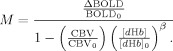
In the hyperoxia method, subjects inhale high levels of oxygen (typically 50–100% O₂ with balance nitrogen where applicable) during acquisition of BOLD image series and recordings of expired oxygen concentration (a surrogate for the arterial partial pressure of O₂). The enriched O₂ raises the total oxygen content of the arterial blood, leading to increases in venous hemoglobin saturation SV_O2) and hence increases in BOLD signal. The maximal BOLD signal M can then be extrapolated using the hyperoxia calibration model of BOLD as a function of SV_O2, with an approximated correction for the small decreases in CBF known to occur during hyperoxia [Chiarelli et al., 2007b; Goodwin et al., 2009; Mark et al., 2011]. Because of the difficulty of measuring small CBF changes with the somewhat noisy ASL method, a fixed value for the hyperoxia‐induced CBF decrease is generally assumed.

The hyperoxia model [Chiarelli et al., 2007b] can be generalized for arbitrary changes in cerebral blood flow during hyperoxia [Gauthier et al., 2011], rendering it valid for conditions such as simultaneous hyperoxia and hypercapnia (as would be produced during breathing of carbogen, a mixture composed largely of O₂ with a balance of 5–10% CO₂). This article presents a detailed description of this generalized calibration model (GCM), examines the sensitivity of the different methods to errors in CBF measurement, and compares values of visually evoked CMRO₂ change obtained using the different calibration approaches.

Theory

Oxygen is a mild vasoconstrictor, and hyperoxia during inhalation of 100% O₂ has been associated with small reductions in cerebral blood flow [Bulte et al., 2007]. The hyperoxia calibration method introduced by Chiarelli et al. [2007b], was thus derived for conditions where cerebral blood flow would be expected to undergo little or no change. To generalize the model to be valid under an arbitrary change in cerebral blood flow, Eq. (12) in Chiarelli et al. can be replaced with the following expression:

(1)

where, as in Chiarelli et al., CBF is the cerebral blood flow in milliliters per second, Cv_O2 is the venous oxygen content in milliliters of O₂ per deciliter of blood, Ca_O2 is the arterial oxygen content (also in ml O₂/dl blood), and OEF is the oxygen extraction fraction (dimensionless, and assumed here to be 0.3 as in Chiarelli et al.). The subscript “0” is used to denote resting values for Ca_O2, OEF, and CBF. The value OEF₀ used in this equation reflects the resting value, which is assumed to be constant throughout the brain and across individuals [Ashkanian et al., 2008; Bremmer et al., 2010; Frackowiak et al., 1980; Ito et al., 2004; Sedlacik et al., 2010]. Whereas the expression proposed by Chiarelli et al. balances O₂ concentrations, the new expression balances the temporal fluxes of O₂ at the level of the capillaries. The above expression can be readily solved for the venous O₂ content during an arbitrary change in blood flow and oxygenation:

(2)

Values for Ca_O2 at baseline and during the breathing manipulations are obtained using the end‐tidal O₂ measurements as in Chiarelli et al. End‐tidal O₂ values are used here as a surrogate for Pa_O2, the arterial partial pressure of O₂. The total arterial O₂ content during carbogen inhalation is obtained from Eq. (11) of Chiarelli et al.:

(3)

where φ is the O₂ carrying capacity of hemoglobin (1.34 ml_O2/g_Hb), [Hb] is the concentration of hemoglobin in blood (15 g_Hb/dl), Sa_O2 is the hemoglobin saturation, and ε represents the solubility of O₂ in plasma (0.0031 ml_O2/(dl_blood × mm Hg)). The constants used here are the same as those in Chiarelli et al. The measured end‐tidal O₂ values were considered equivalent to Pa_O2, and used to determine Sa_O2 using the Severinghaus equation:

(4)

The value for Ca_O2|₀, used above in Eq. (2), is determined using the Pa_O2 value at normoxia, the OEF₀ value of 0.3 is assumed from literature, and the baseline‐normalized CBF value is measured during pCASL imaging.

As a penultimate step, we can estimate the venous O₂ saturation using Eq. (14) from Chiarelli et al. (assuming that plasma O₂ content in venous blood is zero as long as there is any dHb available for binding) and the Cv_O2 value computed above:

(5)

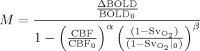
We can now estimate an M value based on values for Sv_O2, BOLD signal increase, and CBF increase during simultaneous hypercapnia and hyperoxia. With variable CBF incorporated explicitly in our revised expression for Cv_O2, we no longer need the CBF correction term “C” from Eq. (8) in Chiarelli et al., and the expression becomes:

(6)

where the term (CBF/CBF₀)^α is used to model cerebral blood volume, assuming α = 0.38 [Grubb et al., 1974], and β = 1.5 is used to model the influence of deoxygenated hemoglobin on transverse relaxation [Boxerman et al., 1995]. The above expression can be readily solved for M:

(7)

Calculation of relative CMRO₂ during a task can then be performed using the expression proposed by Davis et al. [1998]:

(8)

A detailed theoretical comparison of the different models is given in the Appendix.

METHODS

Acquisitions were conducted in eight healthy subjects (seven male and one female, aged 21–38 years) on a Siemens TIM Trio 3T MRI system (Siemens Medical Solutions, Erlangen, Germany) using the Siemens 32‐channel receive‐only head coil for all acquisitions. All subjects gave informed consent and the project was approved by the Comité mixte d'éthique de la recherche du Regroupement Neuroimagerie/Québec.

Image Acquisition

Sessions included an anatomical, 1 mm³ MPRAGE acquisition with TR/TE/alpha = 2,300 ms/3 ms/9°, 256 × 240 matrix and a GRAPPA acceleration factor of 2 [Griswold et al., 2002].

Functional image series were acquired using a dual‐echo pseudo‐continuous arterial spin labeling (pCASL) acquisition [Wu et al., 2007] to measure changes in cerebral blood flow (CBF). The parameters used include: TR/TE1/TE2/alpha = 3,000 ms/10 ms/30 ms/90° with 4 × 4 mm² in‐plane resolution and 11 slices of 7 mm (1 mm slice gap) on a 64 × 64 matrix (at 7/8 partial Fourier), GRAPPA acceleration factor = 2, post‐labeling delay = 900 ms, label offset = 100 mm, Hanning window‐shaped RF pulse with duration/space = 500 μs/360 μs, flip angle of labeling pulse = 25°, slice‐selective gradient = 6 mT m⁻¹, tagging duration = 1.5 s [Wu et al., 2007].

In one subject, five susceptibility‐weighted images (SWI) [Rauscher et al., 2005; Reichenbach et al., 2001] were obtained to provide a qualitative assessment of the venous oxygenation increase with each breathing manipulation. One image was acquired during inhalation of, respectively: air, 7% CO₂/93% air (HC), 100% O₂ (HO), 7% CO₂/93% O₂ (HO‐HC 7%), and 10% CO₂/90% O₂ (HO‐HC 10%). For all images, the acquisition was started after an initial 1‐min period of gas breathing to allow oxygen saturation and vasodilation to reach a plateau. Parameters used for the SWI acquisition were: TR/TE/alpha = 27 ms/20 ms/15° with 0.9 × 0.9 mm² in‐plane resolution with 56 slices of 1.5 mm on a 256 × 192 matrix.

Manipulations

Each session consisted of four functional runs: one run with visual stimulation and three runs each including a different gas manipulation. During each gas manipulation run, a single 3‐min block of gas inhalation was preceded with 1 min and followed by 2 min of medical air breathing. The three gas manipulations used were: 100% O₂ (hyperoxia, or HO), 7% CO₂/93% air (hypercapnia, or HC) and 7% CO₂/93% O₂ (simultaneous hyperoxia and hypercapnia, or HO‐HC). The latter gas is a specific formulation of carbogen, which in general may contain different O₂/CO₂ ratios.

Visual stimulus

The visual stimulus used was a black and white radial checkerboard, with annuli scaled logarithmically with eccentricity, luminance modulated in a temporal squarewave at 8 Hz (equivalent to 16 contrast reversals per second) presented using an LCD projector (EMP‐8300, Epson, Toronto, ON, Canada) onto a translucent screen viewed by subjects through a mirror integrated into the Siemens head coil. This stimulation was initiated 1 min into the acquisition and lasted 3 min, followed by 2 min of rest.

Gas manipulations

At the beginning of the experiment, subjects were fitted with a nonrebreathing face mask (Hudson RCI, #1059, Temecula, CA). To avoid discomfort from outward gas leakage blowing into the subject's eyes, skin tape (Tegaderm Film, #1626W, 3M Health Care, St‐Paul, MN) was used to seal the top of the mask to the face. Plastic tubing (Airlife^TM Oxygen tubing #001305, Cardinal Health, McGraw Park, IL) and a series of two Y‐connectors were used to connect pressure/flow‐meters for medical air, 100% O₂ (hyperoxia, or HO), 7% CO₂/93% air (hypercapnia, or HC) and 7% CO₂/93% O₂ (simultaneous hyperoxia and hypercapnia, or HO‐HC) tanks (Vitalaire, Missisauga, ON, Canada) to the mask. Gas flows were adjusted manually on the pressure/flow‐meters (MEGS, Ville St‐Laurent, QC, Canada) to keep a total flow rate of 16 L min⁻¹. Gas flow was kept at 16 L min⁻¹ at all times except during administration of the HO‐HC and the HC gas mixtures. To accommodate the hyperventilation caused by CO₂ breathing, gas flow rates were increased to the maximal possible rate (25 L min⁻¹) achievable with our pressure/flowmeters. Pulse rate and arterial O₂ saturation were monitored in all subjects using a pulse‐oximeter (InVivo Instruments, Orlando, USA) as a safety measure and to observe the effects of carbogen breathing.

End‐tidal O₂ and CO₂ values were monitored during all acquisitions. Gases were sampled via an indwelling nasal cannula (Airlife^TM Nasal Oxygen Cannula #001321, Cardinal Health, McGraw Park, IL) using the CO2100C and O2100C modules of the MP150 BIOPAC physiological monitoring unit (BIOPAC Systems, Goleta, CA). Calibration of the unit was done by taking into account an expired partial pressure of water of 47 mm Hg [Severinghaus, 1989]. Subjects were instructed to breathe through their nose, which ensured that only expired gas was sampled by the nasal cannula. End‐tidal CO₂ and O₂ values were selected manually from continuous respiratory traces sampled at 200 Hz. The first 10 breaths of the first baseline period and the last 10 breaths of the gas‐inhalation block were averaged to give baseline values and gas manipulation values, respectively.

Following acquisition, all subjects were debriefed to assess the level of discomfort associated with the manipulation. The subjects were asked to rate the air hunger and breathing discomfort associated with the HO‐HC and HC mixtures on a french language version of the scale proposed by Banzett et al. [1996].

Data Analysis

Individual subject analyses for ROI quantifications, absolute CBF, M and CMRO₂ mapping were done using the NeuroLens data analysis software package (http://www.neurolens.org). Time‐series data from each echo were motion corrected [Cox et al., 1999] and spatially smoothed with a 6‐mm 3D Gaussian kernel. ASL data were similarly processed, and the CBF signal was isolated from the first echo (TE = 10 ms) through surround subtraction using linear interpolation between neighboring points [Liu et al., 2005]. A BOLD time series was isolated through surround addition using linear interpolation of neighboring points of the second echo (TE = 30 ms). A general linear model (GLM) including a single‐block response, a linear drift, and constant offset terms was applied, to obtain effect sizes and T‐maps for each condition. The first 60 s after each transition in gas composition were excluded from the analyses by zeroing out relevant rows in the GLM computational matrices, to select responses at (or close to) steady‐state.

Fractional changes were then calculated by dividing effect sizes over the visual ROI by the constant DC term from the GLM averaged within the same region. Group average values ± standard deviation are reported.

Uncertainties on the estimates for M and CMRO₂ were computed through numerical propagation of errors. This was performed by evaluating M and CMRO₂ for all combinations of input values evaluated at the upper and lower bounds of their respective confidence intervals (based on ± SE). The resultant ranges of M and CMRO₂ values were then taken as the uncertainty for the respective parameter.

Absolute CBF maps were generated as in [Wang et al., 2003]. A binary mask was generated from the absolute flow map to remove all voxels with an absolute baseline CBF below 25 mL/100 g/min, as a means of selecting cortical gray matter. Percent CBF and BOLD maps in response to the breathing manipulations as well as the visual task were multiplied by this mask to exclude white matter and CSF, as the low resting CBF levels in these tissue compartments preclude stable estimation of fractional CBF changes required by the model.

Arterial spin‐labeling measurements acquired during hyperoxia alone and combined hyperoxia and hypercapnia were corrected for T1 changes using the approach described in [Chalela et al., 2000; Zaharchuk et al., 2008]. Arterial blood T1 values were estimated based on measured P ${}_{\text{ETO}{}_{\text{2}}}$ (partial end‐tidal pressure of O₂) values for each subject and T1 vs. P ${}_{\text{ETO}{}_{\text{2}}}$ values tabulated in Bulte et al. [2007]. Because the T1 depends specifically on the level of dissolved O₂ in the plasma, and since we obtained different Pa_O2 (arterial partial pressure of O₂) values at a given Fi_O2 (fraction of inspired O₂) than the latter study (their Pa_O2 values were higher, likely due to the use of a tightly sealed face mask), the values were interpolated to account for this difference (i.e., the table from Bulte et al. was converted to T1 vs. group average Pa_O2, and the T1 corresponding to each subject's P ${}_{\text{ETO}{}_{\text{2}}}$ during hyperoxia manipulations was interpolated). Values for the absolute blood flow at the air‐breathing baseline were computed using Eq. (1) from Wang et al. [2003], assuming the same constant values as in this reference.

The resultant values of percent change in ASL and BOLD signals (and where appropriate P ${}_{\text{ETO}{}_{\text{2}}}$) were input to the applicable BOLD signal models to generate maps of the M parameter. More specifically, ASL and BOLD responses during hypercapnia were input to the hypercapnia model [Davis et al., 1998], while BOLD, and P ${}_{\text{ETO}{}_{\text{2}}}$ data were input to the hyperoxia model [Chiarelli et al., 2007b] with an assumed flow decrease of 5% (based on P ${}_{\text{ETO}{}_{\text{2}}}$ values obtained in our subjects and the flow decrease observed by Bulte et al. for similar P ${}_{\text{ETO}{}_{\text{2}}}$ levels [Bulte et al., 2007]. The generalized calibration model (GCM) was applied to ASL, BOLD, and P ${}_{\text{ETO}{}_{\text{2}}}$ data for all manipulations.

Visual

Regions of interest (ROIs) were derived from the intersection of the flow and BOLD thresholded (P = 0.01 corrected), [Worsley et al., 2002] visual activation T‐maps for each individual subject from the NeuroLens analysis. One subject (Subject 1) fell asleep during the visual task and was therefore excluded from all analyses requiring a visual ROI.

Gray matter

A gray matter ROI was defined for each subject using the automatic tissue segmentation functionality of the CIVET software package [Tohka et al., 2004].

Analysis of sensitivity to errors in CBF

One of the limiting factors in the application of calibrated MRI methods has been the low signal‐to‐noise ratio of ASL measurements. To assess the sensitivity of different M estimation methods to possible errors in cerebral flow change, we computed M values based on group average ROI and respiratory measures with simulated errors in the gas‐induced CBF response. In these simulations, the input value of baseline‐normalized CBF was varied over a range corresponding to the measurement uncertainty exhibited by our data while other input parameters (BOLD response and, where applicable, end‐tidal O₂ values) were held constant. This computation was carried out for the Davis model with HC data, for the Chiarelli model with HO data, and for the GCM with HC, HO, and HO‐HC data.

RESULTS

End‐tidal partial pressures of O₂ (P ${}_{\text{ETO}{}_{\text{2}}}$) and CO₂ (P ${}_{\text{ETCO}{}_{\text{2}}}$) achieved during each gas manipulation for each subject are shown in Table I. While P ${}_{\text{ETCO}{}_{\text{2}}}$ values were very similar between HC and HO‐HC, P ${}_{\text{ETO}{}_{\text{2}}}$ values tended to be lower for HO‐HC than for HO alone (possibly reflecting the 90% vs. 100% O₂ content of the two gases). The changes in blood oxygenation resulting from these three gas manipulations can be appreciated from the ROI‐average values for BOLD signal change (Fig. 1B), while the vasodilatory effect of CO₂ is demonstrated by the CBF changes within the same ROIs (Fig. 1A). Percent changes in CBF (Fig. 1A) for HC and HO‐HC were not found to be significantly different (paired two‐tailed Student's t test, P > 0.3) in both visual and GM ROIs. Average CBF changes in the visual ROI were 63.3% ± 6.7% and 68.9% ± 12.2%, while average changes throughout GM were 37.3% ± 4.8% and 40.7% ± 3.7% for HC and HO‐HC, respectively. Average flow changes for HO in visual and GM ROIs were, respectively, ‐7.3% ± 3.7% and ‐3.1% ± 3.1%. BOLD percent changes (Fig. 1B) for HC and HO were similar, with averages of 2.3% ± 0.2% and 1.9% ± 0.2% in the visual ROI and 2.3% ± 0.1% and 1.7% ± 0.2% in GM for HC and HO, respectively. Average ROI values for HO‐HC were about double those of HO and HC alone, with averages of 4.1% ± 0.4% and 3.6% ± 0.4%, respectively for visual and GM ROIs.

Table I.

End‐tidal values for each breathing manipulation

	Subject	Subject	Subject	Subject	Subject	Subject	Subject	Subject
	1	2	3	4	5	6	7	8	Average
P ${}_{\text{ETCO}{}_{\text{2}}}$ baseline	37.7	41.7	38.3	41.9	39.3	42.0	40.4	34.5	39.5
P ${}_{\text{ETCO}{}_{\text{2}}}$HC	51.2	52.2	47.5	46.9	51.9	46.9	47.8	42.3	48.3
P ${}_{\text{ETO}{}_{\text{2}}}$ baseline	113.9	114.1	113.0	139.0	125.4	125.0	92.3	106.3	116.1
P ETO 2HO	578.4	621.6	509.3	569.8	583.6	380.0	560.8	513.1	539.6
P ${}_{\text{ETCO}{}_{\text{2}}}$ baseline	41.8	42.0	37.2	40.8	41.2	41.3	40.1	35.1	40.0
P ETCO 2HO‐HC	48.9	51.0	46.1	46.9	50.8	46.7	45.9	45.5	47.7
P ${}_{\text{ETO}{}_{\text{2}}}$ baseline	102.9	104.0	135.7	125.2	114.0	130.3	106.4	105.4	115.5
P ${}_{\text{ETCO}{}_{\text{2}}}$HO‐HC	447.5	480.8	400.8	425.1	486.7	303.8	403.5	375.6	415.5

Average end‐tidal values for individual subjects. The top subsection shows end‐tidal partial pressures of CO2 (P _{ETCO 2}) for the hypercapnia (HC) breathing manipulation during baseline (top row) and during the hypercapnia block (second row). The second subsection shows end‐tidal partial pressures of O2 (P _{ETO 2}) for the hyperoxia (HO) breathing manipulation during baseline (third row) and during the hyperoxia blick (fourth row). The third section shows (P _{ETCO 2}) and (P _{ETO 2}) (baseline and block) for combined hypercapnia and hyperoxia (HO‐HC).

Figure 1.

Group average percent CBF and BOLD for each breathing manipulation. Group average percent CBF (A) and percent BOLD (B) changes over visual and gray‐matter ROIs for hyperoxia (HO), hypercapnia (HC), and combined hypercapnia and hyperoxia (HO‐HC).

Individual subjects' ROI‐based M values for visual cortex are summarized in Figure 2A and Table II. Values of M are shown for each gas manipulation (HC, HO, and HO‐HC), calculated with the original model for that manipulation. Group average M values were 5.6% ± 1.8%, 4.5% ± 1.5%, and 7.6% ± 2.6% for HC, HO, and HO‐HC, respectively over the visual ROI. The M values estimated using the HO‐HC technique were generally found to be the highest, while HO tended to give the lowest values. Application of the GCM to ROI‐average CBF and BOLD signals as well as P ${}_{\text{ETO}{}_{\text{2}}}$ values measured during hypercapnia yielded slightly lower values than those of the Davis model (M values with GCM were on average lower by 0.5% ± 0.2%). On the other hand, application of the GCM to the BOLD and P ${}_{\text{ETO}{}_{\text{2}}}$ values recorded during hyperoxia (with an assumed flow decrease of 5%) yielded systematically higher M values than the Chiarelli model (M values with GCM were on average 1.7% ± 1.1% higher; data not shown).

Figure 2.

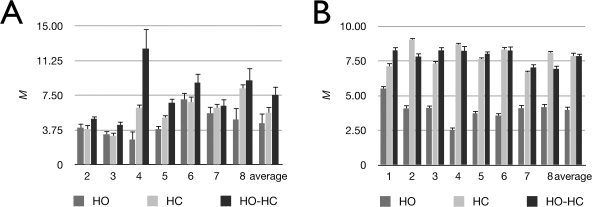
Individual and average M values over the visual and gray‐matter ROIs for each breathing manipulation. Individual and group average M values over visual (A) and gray‐matter (B) ROIs for hyperoxia (HO), hypercapnia (HC), and combined hypercapnia and hyperoxia (HO‐HC). The Chiarelli, Davis and GCM formulae were used to process data from the respective gas manipulations.

Table II.

Calibrated fMRI results

	Subject	Subject	Subject	Subject	Subject	Subject	Subject
	1	2	3	4	5	6	7	Average
Reactivity HC	6.5	8.5	8.3	6.0	8.7	10.7	6.1	7.8
Reactivity HO‐HC	9.3	10.3	2.3	8.3	8.4	10.1	2.9	7.4
M HC	3.8	3.1	6.1	5.1	6.8	6.2	8.3	5.6
M HO	4.0	3.3	2.7	3.9	7.1	5.6	4.9	4.5
M HO‐HC	5.0	4.3	12.6	6.7	8.9	6.4	9.1	7.6
CMRO2 HC	26.5	6.7	7.9	28.2	28.2	40.8	36.8	25.0
CMRO2 HO	27.3	8.7	−30.8	21.6	29.1	36.1	25.6	16.8
CMRO2 HO‐HC	31.6	17.5	21.7	32.9	33.1	42.3	38.3	31.1
n HC	2.7	9.4	6.1	2.4	2.5	3.0	2.0	4.0
n HO	2.6	7.2	−1.6	3.2	2.4	3.4	2.9	3.0
n HO‐HC	2.2	3.6	2.2	2.1	2.1	2.9	2.0	2.4

Individual subjects' and average values for vascular and metabolic parameters. The first section shows vascular reactivity (% change CBF/mm Hg change in P ${}_{\text{ETCO}{}_{\text{2}}}$) values for hypercapnia (HC) and combined hypercapnia and hyperoxia (HO‐HC). The second section shows average M values over the visual ROI for each breathing manipulation. The third section shows estimates of visually evoked CMRO₂ using M values calculated with the M value associated with each breathing manipulation. Finally, the fourth section shows the coupling constant between CBF and CMRO₂ associated with the estimates obtained from each breathing maniplation.

Some similarities were observed when M was estimated over all gray matter (Fig. 2B). Group average M values were 7.9% ± 0.8%, 4.0% ± 0.8%, and 7.9% ± 0.6% for HC, HO, and HO‐HC, respectively. The tendency toward higher M values with HO‐HC and lower M values with HO is clearer here with a lower intersubject variability. Application of the GCM to data obtained during HC yielded lower M values than the Davis model (values computed with GCM were on average 0.8% ± 0.3% lower than those from the Davis model). On the other hand, M values estimated using the GCM during HO were higher than those obtained using the Chiarelli model (1.3% ± 0.4% higher for GCM as compared to the Chiarelli model; data not shown).

Maps of M for each breathing manipulation using the model originally derived for the respective procedures are shown in Figure 3. A similar pattern may be observed between subjects whereby HO yields lower and more uniform maps of M values, with few localized enhancements compared to HC and HO‐HC. The maps created using HC show a speckled pattern of focal M hotspots, some of which appear (based on placement with respect to sulcal anatomy) to be veins, while others appear artifactual, likely from instabilities in the model under high CBF errors (Fig. 4). Maps from HO‐HC exhibit an intermediate pattern with more uniform M values throughout cortex combined with local enhancements associated with larger veins. The reduced prevalence of questionable hot spots in the HO‐HC maps, as compared to the HC maps can be appreciated in the example maps shown in Figure 4. In this figure, the window display levels were adjusted to highlight the differences in the high amplitude local enhancements in these maps, as opposed to the scale used in Figure 3, chosen to show general trends over all techniques and subjects.

Figure 3.

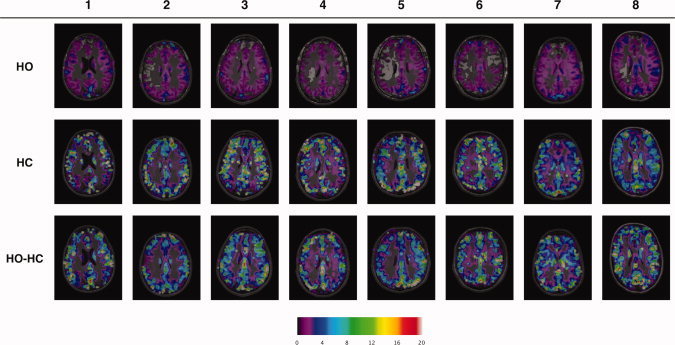
Individual M maps for each breathing manipulation. Individual M maps for hyperoxia (HO) (top row), hypercapnia (HC) (second row) and combined hypercapnia and hyperoxia (HO‐HC) (third row). The Chiarelli, Davis, and GCM expressions were used to process data from the respective gas manipulations. Display window levels have been adjusted to emphasize detail in all maps.

Figure 4.

Spatial heterogeneity of M maps. Maps of M from one subject for HC and HO‐HC (using Davis model and GCM, respectively). The display window levels have been adjusted to highlight the differences in the magnitude of M estimates within local enhancements.

The susceptibility‐weighted venograms acquired in one subject provide a qualitative depiction of the venous saturation provided by each breathing manipulation (Fig. 5). In this subject, the prominent veins visible in the baseline image acquired during air breathing can be seen to fade due to increasing levels of oxygen saturation for 100% O₂ (HO) breathing and 7% CO₂/93% air (HC) mixtures. While a carbogen mixture with 10% CO₂/90% O₂ (HO‐HC 10%) composition yields a complete loss of venous contrast, the carbogen mixture with 7% CO₂/93% O₂ (HO‐HC 7%) shows an intermediate pattern with complete loss of venous contrast in smaller veins, but some residual contrast in the largest veins.

Figure 5.

Susceptibility‐weighted venograms during each breathing manipulation. Susceptibility‐weighted venograms acquired in a single subject during breathing of either air, 100% O₂ (HO), 7% CO₂/93% air (HC), 7% CO₂/93% O₂ (HO‐HC 7%) and 10% CO₂/90% O₂ (HO‐HC 10%).

Simulations of the effect of CBF error on apparent M value are shown in Figure 6. Estimates of M based on manipulations including hypercapnia exhibited greater‐than‐linear increases in the error on M as a function of CBF underestimation (for both Davis model and GCM). However this nonlinearity and resultant errors on M were far smaller, over the entire range of CBF errors examined, for GCM in combination with HO‐HC than for other methods (Fig. 6A). Estimates of M based on hyperoxia alone exhibited marked instabilities for relatively small errors in CBF (for both the Chiarelli model and GCM) (Fig. 6B).

Figure 6.

Effect of CBF errors on M estimates from different models and breathing manipulations. Solid lines show M estimates as a function of the error in CBF, while the broken lines (nearly overlapping) show the values of the actual M estimates from the group average visual ROI flow response (i.e., without error) for the different methods. All estimates use group average values for BOLD and respiratory measures, as well as for the central (zero error) value of CBF. For manipulations and models with a HC component (A), HC/Davis, HC/GCM and HO‐HC/GCM, greater‐than‐linear error occurs with progressive underestimation of the flow response to hypercapnia. The combination of HO‐HC with the GCM yielded M estimates with the greatest immunity to errors in CBF. The hyperoxia‐only manipulation, when used with either the GCM and Chiarelli model (B) shows a singularity at flow estimates within the typical error bounds on ASL measurements.

Percent changes in CMRO₂ over visual cortex were computed for each subject using ROI‐average values for CBF and BOLD increases during the visual task and M values obtained from each breathing manipulation (Fig. 7 and Table II). While group average values for each technique were similar and a pattern for large intersubject variability can be seen, some patterns nevertheless emerge from this analysis. The HO‐HC technique yielded physiologically plausible estimates of relative CMRO₂ change in all subjects. HC, on the other hand, yielded very low and nonphysiological Δ%CMRO₂ estimates in two subjects (subjects 2 and 3 in Fig. 7). HO also resulted in a nonphysiological, negative Δ%CMRO₂ estimate in one subject (subject 3 in Fig. 7).

Figure 7.

Individual and average CMRO₂ estimates over the visual ROI. Individual and group average evoked CMRO₂ estimates for the visual task, calculated using M values from hyperoxia (HO), hypercapnia (HC) and combined hypercapnia and hyperoxia (HO‐HC) manipulations (and respective models).

Calibrated fMRI parameters, including cerebrovascular reactivity during HC and HO‐HC, M, CMRO₂ and the coupling parameter n are shown for each subject in Table II. Vascular reactivities were similar in most subjects for HC and HO‐HC, except in Subjects 3 and 7, who exhibited lower flow responses to HO‐HC than to HC alone. The coupling constant n is defined here as the magnitude of the fractional flow change during a stimulus divided by the corresponding fractional change in CMRO₂. Values for n are expected to be between 2 and 4 (Buxton 2010). While most n values fall within this range, some values obtained using either HC or HO calibration exhibited physiologically suspect values with either very high (Subjects 2 and 3) or one negative value (Subject 3) in the case of HO calibration.

DISCUSSION

Estimation of M Parameter

Comparison of functional MR calibration methods based respectively on hypercapnia, hyperoxia, and combined hypercapnia and hyperoxia indicates that the hybrid technique may yield more robust and accurate M estimates thanks to the reduced range of extrapolation required from the higher measured BOLD signals. In the latter assessment we define robustness as the relative immunity from physically invalid results such as negative, imaginary, or artifactually large values, and accuracy in terms of agreement with the lower bound on M values set by previous direct measures in which high levels of venous saturation were produced. Estimates of M based on HO‐HC show a trend toward higher values than the individual HC and HO approaches (the latter yielding the lowest values).

ROI Analysis

Group average M values obtained with the HO‐HC method in visual cortex (7.6 ± 2.8) were similar to the average value of 7.5 ± 1.0 measured directly in a previous study using simultaneous hypercapnia and hyperoxia with a higher CO₂ content (10% CO₂/90% O₂) to reach very high venous O₂ saturation from a larger flow response [Gauthier et al., 2011]. The value of 7.5% BOLD signal increase measured in Gauthier et al. can be considered a direct measurement of (or at least a lower bound on) M, as venous saturation levels exceeding 90% were reached in this experiment. Both the HC and HO calibration techniques, on the other hand, yielded M estimates of 5.6 ± 1.8 for HC and 4.5 ± 1.5 for HO, well below the directly measured lower bound for M cited above. The agreement between directly measured BOLD signal changes at very high venous saturations and the M value extrapolated here from the smaller HO‐HC changes provided by the 7%CO₂/93%O₂ carbogen mixture used here indicates that the values obtained with this technique may be more accurate.

The accuracy of M has been shown to have an important impact on the validity of task‐induced CMRO₂ responses estimated through calibrated MRI [Chiarelli et al., 2007a]. The higher BOLD signal values obtained from the combined sources of increased oxygen saturation and the larger (and thus more readily measurable) flow values obtained from the 7% CO₂ content reduce the range of extrapolation required to estimate the maximal BOLD response.

Susceptibility‐Weighted Venograms

The distance of measured BOLD responses from (or their proximity to) the maximal BOLD signal change can be demonstrated qualitatively by SWI venograms acquired during the different breathing manipulations. In one subject we acquired venograms during breathing of the following gases: air, 100% O₂ (HO), 7%CO₂/93% air (HC), 7% CO₂/93% O₂ (HO‐HC 7%) and 10% CO₂/90% O₂ (HO‐HC 10%), (Fig. 5). This last mixture, 10% CO₂/ 90% O₂ has been shown in previous studies [Gauthier et al., 2011; Sedlacik et al., 2008] to yield an almost complete loss of venous contrast in SWI due to a very large increase in venous oxygenation. This supports use of the BOLD change produced by this manipulation as a direct measurement of M and a ground truth against which to compare other manipulations (including carbogen breathing at lower CO₂ levels). The SWI venograms in Figure 5 demonstrate different degrees of reduced susceptibility contrast in veins, with the effect of HO‐HC at 7% CO₂ exceeding those of HC or HO alone by a considerable margin. The venogram acquired during HO‐HC at 10% CO₂ demonstrates a complete loss of susceptibility contrast.

M mapping

Estimates of M have, in the past, typically been expressed as average values over regions of interest. Here we show maps of M values over all voxels in which an absolute baseline CBF above 25 mL/100g/min was measured (chosen to exclude CSF and white matter), allowing an investigation into the spatial distribution of M values.

Maps of M obtained from the hypercapnia manipulation included numerous isolated voxels with very high M values (Figs. 3 and 4). While M values in larger veins are expected to be high, some of these high values obtained with this approach appear to be artifactual. This may be due to amplification of noise inherent in the broad range over which extrapolation is required, as well as an inherent instability of the model for low flow estimates (see Appendix and Fig. 6). Maps of M generated using hyperoxia alone with the hyperoxia model (Fig. 3) showed a tendency toward lower M values and appeared to underestimate the values in larger veins (which were essentially absent in the maps). Note that many of the hyperoxic M maps included large zones in which the gray‐matter M was negative, which are shown as fully transparent in the image overlays of Figure 5.

Spatial heterogeneity of M values

Mark et al. have compared the hypercapnia and hyperoxia manipulation techniques. They found the M values obtained with the hyperoxia technique to show less intersubject variability than hypercapnia. Given that the hyperoxia technique assumes a fixed flow value in response to hyperoxia and a uniform venous saturation based on end‐tidal PO₂ measurements, the main contribution to noise comes from the BOLD measurement. The hypercapnia method, on the other hand, uses the noisier flow response to hypercapnia in its model.

Though the greater uniformity of hyperoxia‐derived M values could be viewed as an advantage, it may in fact reflect bias in the technique—particularly where large veins are concerned. It is known a priori that veins must have a higher M value than parenchyma, since their dHb content is higher. Such veins do in fact show higher BOLD increases than gray matter during hyperoxia, but application of the hyperoxia model results in M values considerably below those detected using the other techniques. This may be due to the assumption of a single fixed flow change throughout the brain, or a breakdown of the model in regions with a high venous blood volume fraction.

The M parameter maps generated from the combined hypercapnia–hyperoxia manipulation with GCM analysis accurately captured the high M values in large veins while remaining free of the artifactual hot spots due to model instability seen in the hypercapnia maps and the zones of negative M value observed in the hyperoxia maps.

Robustness of M estimates

As noted above, maps of M generated using the GCM in conjunction with the HO‐HC manipulation appeared to be relatively immune to artifactual hot spots compared with maps generated using the Davis model and the hypercapnia manipulation. Detailed analysis of M maps together with input maps of CO₂‐induced BOLD and CBF responses indicated that improbably high M values in the Davis/HC maps tended to occur in voxels where the apparent CBF change was atypically low compared with surrounding voxels. Such low flow values in individual voxels may reflect a combination of noise excursions from the “true” gray‐matter value and bias caused by partial volume with white matter or large veins. The simulation results presented in Figure 6 reveal that estimates of M exhibit nonlinear errors for increasing errors in CBF. The degree of error was found to depend both on the model used and the gas manipulation employed.

Both the Davis model and the GCM can be used to compute M from data acquired during hypercapnia. Simulation results indicated that hypercapnic M estimates using the GCM were somewhat more stable (i.e., nonlinearity of the error in M was reduced) than those obtained using the Davis model (Fig. 6A). This is due to the moderating effect of terms in the GCM reflecting arterial O₂ content at rest and during hypercapnia. While the details of this are presented in the appendix, it is interesting to note that incidental increases in arterial PO₂ from CO₂‐induced hyperventilation actually tend to stabilize estimates of M derived from hypercapnic measures with the GCM.

Data acquired during pure hyperoxia can be analyzed using either the Chiarelli model or the GCM. Although the Chiarelli model is often applied using an assumed value of the O₂‐induced CBF decrease, it was important to assess the impact of any misassignment of this parameter (whether through measurement error or incorrect assumption). Our simulations showed that relatively modest errors in the O₂‐induced CBF change could result in extremely large bias in the apparent M value (culminating in singularities at CBF errors well within the typical standard deviation). This was the case for both the Chiarelli model and the GCM formulation, although the specific range of CBF errors where singularity arose was different for the two models (Fig. 6B). As discussed in the Appendix, this instability is due to the lower range of flow values obtained in the hyperoxia manipulation, which fall in regimes for both models where division by zero can readily occur with typical values of other parameters. It should be noted that practical applications of the hyperoxia approach typically use a fixed value for the O₂‐induced decrease in CBF that lies within the stable range for both models.

The simulation results for the GCM in conjunction with the combined hypercapnia/hyperoxia manipulation demonstrate the relative immunity of this approach to typical errors in CBF. The mathematical basis for this stability is discussed in the appendix, but it can also be understood on intuitive grounds by considering that, in the limit, complete saturation of venous blood would completely eliminate the dependence of M on the CBF and CBV terms. Because the combined effects of simultaneous hypercapnia and hyperoxia drive the venous system considerably closer to this endpoint than other manipulations, and because the GCM is valid for such simultaneous manipulations, it offers improved accuracy and robustness in the estimation of M over previous methods.

CMRO₂

The M parameters obtained using each breathing manipulation were used as intermediate results in the estimation of fractional CMRO₂ changes evoked during a visual task. While most CMRO₂ estimates fell within the range reported in the literature for similar visual paradigms [Ances et al., 2008; Davis et al., 1998; Hoge et al., 1999a; Leontiev et al., 2007a, b; Lin et al., 2008; Perthen et al., 2008; Stefanovic et al., 2006], some physiologically implausible estimates of CMRO₂ were also calculated using the hypercapnia and hyperoxia calibration methods (Fig. 7, Table II). In Figure 7, Subjects 3 and 4 have either nonphysiological (Subject 4) or atypically low (Subject 3) CMRO₂ responses associated with the visual task. In these two subjects, M values estimated with combined hypercapnia and hyperoxia were larger than those estimated using the other two methods. In the case of subject 3, the M value from HO‐HC was about 1% higher than with the other two methods and this led to the estimation of a CMRO₂ value around 17.5%, much closer to the expected range (between 15 and 35%) than the values of 6.7 and 8.7% found by HC and HO, respectively. In Subject 4, the very high estimate for M obtained by HO‐HC (12.6%) is however the only value for M that, when coupled with the task‐related signal changes in CBF and BOLD, yields a plausible CMRO₂ estimate (21.7% as opposed to 7.9 or ‐30.8% for HC and HO, respectively). Furthermore, this high M value is within the range of values reported in previous studies [Perthen et al., 2008] and is not inconceivable for an individual endowed with unusually prominent venous anatomy.

Limitations of the Study

Breathing manipulations

High inspired CO₂ concentrations are known to be associated with air hunger and dyspnea [Banzett et al., 1996]. In the present study, we used 7% CO₂ for both the HC and HO‐HC conditions. While this CO₂ content is somewhat higher than the 5% CO₂/air mixture often used in the calibrated fMRI literature, it was chosen here to ensure high flow increases and venous saturation levels. The discomfort associated with this CO₂ concentration was, furthermore, found to be mild with an average discomfort rating of 2.1 ± 0.6 on a seven‐point scale [Banzett et al., 1996]. In the future, the high flow and BOLD signal responses measured with combined hypercapnia and hyperoxia could be utilized, in frail populations, to reduce CO₂ concentrations while achieving sufficient BOLD and ASL signal levels for adequate sensitivity.

Previous studies have, for similar fixed inspired gas concentrations, detected higher end‐tidal values during hyperoxia [Bulte et al., 2007; Chiarelli et al., 2007b] than those reported here. This is probably due to air being entrained into the partially unsealed mask used here, especially during breathing manipulations involving CO₂ and therefore leading to increased minute ventilation. A setup allowing the accommodation of larger breathing volumes and rates (including a mask with a larger bag and flow regulators allowing larger volumes to be given) would allow the mask to be sealed and prevent contamination from room air. This would be desirable as it would provide higher oxygenation increases for the same inspired gas O₂ and CO₂ gas concentrations. However the validity of the methods presented here depends only on the ability to accurately record the evoked changes in end‐tidal O₂ and CO₂, which is ensured by instructing subjects to exhale through their nose and sampling via an indwelling nasal cannula. The requirement for breathing through the nose could be removed in future patient studies using a more closely sealed mask and the use of a one‐way valve to prevent mixing of inspired and expired gases.

M value confounds

The dual‐echo pCASL technique used here gave reliable flow and BOLD estimates in the gray matter that allowed the GCM to provide consistently plausible M values. The relatively higher noise levels in flow and BOLD signal changes measured in white matter voxels however yield clearly invalid estimates of M and CMRO₂. This technique (like the pure hypercapnia and hyperoxia methods) is thus not currently suitable for calculating maximal BOLD signal or CMRO₂ in white matter.

Because of the low spatial resolution, bias in flow and BOLD estimates from partial volume effects is clearly a concern at the interfaces between gray matter and white matter or cerebrospinal fluid. Inspection of the M parameter maps indicates that there is indeed a zone in which M falls smoothly to zero along the gray‐white matter interface. Parameter estimates in regions of homogeneous gray matter are thus likely to be more quantitative. Also, caution is needed when interpreting the M values that appear to fall in pure white matter as seen in Figure 3, since these in fact arise from a partial volume effect of adjacent slices during the resampling of the functional data to the anatomical resolution.

A potential advantage of the combined hyperoxia and hypercapnia calibration is the reduced dependence on the assumptions of a fixed flow‐volume coupling relationship and that CMRO₂ does not change during changes in arterial O₂ or CO₂ levels [Chen et al., 2010a; Hino et al., 2000; Horvath et al., 1994; Jones et al., 2005; Kety et al., 1948; McPherson et al., 1991; Xu et al., 2011; Zappe et al., 2008]. This can be appreciated by considering the limiting case in which concurrent flow and oxygenation increases drive venous O₂ saturation to 100%. Under such conditions, venous blood volume is no longer relevant since venous blood does not contain any deoxygenated hemoglobin. Moreover if venous oxygenation is driven to 100%, this means that all metabolic oxygen consumption has been satisfied by a combination of O₂ carried on hemoglobin and dissolved in blood plasma, regardless of whether CMRO₂ was constant during the calibration. While this is not the case for the submaximal values of venous saturation achieved in the present study, it is clear that the influence on M of systematic errors in the CBV term (estimated from CBF) and CMRO₂ change (assumed to be zero) must become progressively smaller with increasing venous saturation (ultimately having no effect at 100% saturation as mentioned above). The group average venous saturation during combined hyperoxia and hypercapnia in the present study was computed to be 87% ± 4% in visual cortex, leaving relatively little deoxyhemoglobin (∼ 13% desaturation) and thus considerably reducing the impact of venous blood volume. A modest decrease in CMRO₂ caused by the administered CO₂ [Xu et al., 2011] would imply a slightly higher true saturation value, with minimal effect on the computed M value.

In the present study, the model parameters alpha and beta were assigned the same values as in prior calibrated MRI literature (e.g. Davis, Chiarelli), [Chiarelli et al., 2007b; Davis et al., 1998]. While the purpose here was to highlight the different model formulations, it should be noted that recent studies have attempted to refine these parameters to values that more specifically reflect venous blood volume and its regional variations (alpha), and more realistically describe the concentration‐relaxation behavior applicable in gradient‐echo EPI at 3 Tesla (beta), [Buxton, 2010; Chen et al., 2009a, b; Mark et al., 2011]. As noted above, the higher venous saturation values attained during combined HO‐HC reduce the impact of slight misspecifications of alpha and beta.

CONCLUSION

The combined hypercapnia and hyperoxia procedure with the generalized model was found to yield M values that were robust at the individual voxel level and consistent with the lower bound determined in a previous study in which M was determined during near‐complete arterialization of venous blood.

The combined sources of increased venous saturation, in conjunction with the added stability of the GCM over previous models, allow a more robust estimation of M, with a reduced range of extrapolation. We believe that this provides more accurate and robust estimates of stimulus‐evoked increases in CMRO₂ than previous methods.

The Davis, Chiarelli, and generalized models all use the same basic expression, originally derived by Davis, to compute the resting BOLD signal M from CBF and BOLD changes measured during a respiratory manipulation:

(9)

All approaches use Grubb's relation to model the change in venous cerebral blood volume:

(10)

where the exponent α may be assigned a value of 0.38 as in the original Grubb study, or an alternate value to better reflect the venous portion of blood volume [Chen et al., 2009a, b].

Where the models differ is in how they express the baseline‐normalized concentration of deoxygenated hemoglobin (dHb) in Eq. (9). To consider how the models differ, we introduce the variable D to represent this dHb term:

(11)

In the discussion that follows, we will use the term desaturation to describe the fraction of hemoglobin that is deoxygenated (equivalent to one minus the saturation expressed as a decimal fraction). We can now proceed to analyze the different models.

Davis Model With Hypercapnia Manipulation

We start by considering the original Davis model, which was intended for use with data acquired during a hypercapnic manipulation without changes in arterial oxygen tension. In the Davis model, it is assumed that there is no deoxygenated hemoglobin in arterial blood (i.e., arterial O₂ saturation is 100%), and that metabolic oxygen extraction does not change during hypercapnia. In this case the relative level of dHb can be expressed simply as

(12)

That is, doubling CBF will reduce the venous concentration of dHb by a factor of two. There has been considerable discussion of whether oxygen extraction can really be assumed to be constant during hypercapnia [Chen et al., 2010a; Hino et al., 2000; Horvath et al., 1994; Jones et al., 2005; McPherson et al., 1991; Zappe et al., 2008]. Moreover, typical arterial O₂ saturation values in young volunteers are actually slightly less than 100%, and this value could be considerably lower in individuals with impaired cardiopulmonary function (e.g., the elderly, respiratory patients). Finally it is possible that arterial O₂ tension will increase during a hypercapnic manipulation, due to CO₂‐induced hyperventilation.

Chiarelli Model With Hyperoxia Manipulation

The Chiarelli model was conceived for use during a hyperoxic manipulation, during which metabolic oxygen extraction is also assumed constant. In this formulation of the model, the relative concentration of deoxygenated hemoglobin is expressed as the sum of two additive terms:

(13)

where φ is the O₂ capacity of hemoglobin in ml O₂/g Hb, [Hb] represents the concentration of hemoglobin in the blood in g Hb/dl blood, OEF₀ is the oxygen extraction fraction at rest, and Ca_O2 is the total arterial oxygen content in ml O₂/dl blood (determined from measurements of end‐tidal O₂). The above expression groups D into two key terms depending, respectively, on end‐tidal gas measures (B) and cerebral blood flow (C). The term B represents the increase in saturation attributable directly to the rise in arterial O₂ content from breathing the hyperoxic gas mixture, while C reflects variable dilution of venous dHb associated with reduced CBF during hyperoxia.

Generalized Calibration Model (GCM) With Hyperoxia and Hypercapnia

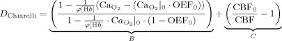
While the expression for D _Chiarelli above is reasonably accurate for the small changes in CBF expected during normocapnic hyperoxia, the GCM incorporates arbitrary CBF changes in a modified version of the B term, resulting in a more general and accurate expression for relative deoxyhemoglobin concentration and obviating the need for term C. With some reorganization, the modified expression that distinguishes the GCM can be expressed as

(14)

In the above expression, the term X is equivalent to the hemoglobin desaturation due specifically to resting metabolism, expressed as a fraction of the total resting hemoglobin desaturation in the venous compartment. It thus serves to modulate the CBF term of the Davis model, accounting for the fact that the arterial O₂ saturation may not be 100% (if resting arterial saturation is 100% then all venous dHb comes from metabolism and the term X reduces to unity).

The term Y, which is equivalent to the hyperoxic arterial desaturation as a fraction of total resting venous desaturation, reflects additional oxygen available from hyperoxic arterial blood for augmenting venous saturation. During hyperoxia, it is possible for the effective arterial desaturation (the numerator in Y) to be negative, which reflects the fact that even at 100% arterial Hb saturation, additional O₂ dissolved in arterial plasma will eventually bind to venous dHb (thus reducing the venous desaturation). If the total arterial O₂ content during the respiratory manipulation corresponds exactly to 100% saturation, then the term Y reduces to zero.

Because the X and Y terms, respectively reduce to unity and zero for a constant arterial O₂ content corresponding exactly to 100% arterial saturation, the GCM is equivalent to the Davis model under the specific assumptions of that model. The GCM is also equivalent to the Chiarelli model in the specific case where there is no change in CBF during hyperoxia.

Stability of the Models During Hypercapnic Manipulations

The largest source of error in estimates of M obtained from hypercapnia data is the high noise level of the CBF measurements. Because all of the models examined here include a CBF term in the denominator of the expression for M, moderate in CBF result in very high errors on M due to the nonlinearity inherent in the reciprocal function. However the degree of nonlinearity and resultant stability under noisy CBF data vary between the different models.

Both the Davis model and GCM can be used to estimate the resting BOLD signal based on measurements during hypercapnia (end‐tidal O₂ measurements are additionally required for the GCM). In the case where end‐tidal O₂ measurements indicate an unchanging arterial saturation of exactly 100%, both models will yield identical results. As illustrated in Figure 6A, the Davis model results in a significant overestimation of M when CBF is sufficiently underestimated. When the GCM is used to analyze the same data, as shown in Figure 6A, the nonlinearity of M with CBF underestimation is considerably less pronounced. This is due to a slight attenuation of the CBF factor in D_GCM from the X term (since resting arterial saturation is slightly less than 100%) and to the damping effect of the additive Y term (which is slightly negative since arterial O₂ content actually increases slightly due to hyperventilation during CO₂ breathing).

This finding has the interesting consequence that small, incidental increases in arterial Pa_O2 during hypercapnia may actually be advantageous (helping to stabilize the model) if they are recorded and input to the GCM. As discussed below, the same effect accounts for the dramatic improvement in estimation stability when the GCM is used in conjunction with simultaneous hypercapnia and hyperoxia.

Note that, while it is theoretically possible to apply the Chiarelli model to measurements of hypercapnically induced changes in CBF, BOLD, and end‐tidal O₂, the resultant estimates of M are physiologically implausible (negative for the input data used here).

Stability of the Models During Hyperoxia Manipulations

Either the Chiarelli model or GCM can be used to compute M from data acquired during a hyperoxic manipulation. Figure 6B indicates that M estimates produced in this way are also vulnerable to significant bias from measurement errors on CBF, regardless of the model used. In this case, the problem arises due to an interaction between the lower range of flow values encountered with the hyperoxia manipulation and the form of the denominator for M in Eq. (9). Moderate excursions in CBF can result in a combination of terms for baseline‐normalized CBV and [dHb] which lead to division by zero. With the Chiarelli formulation, this only occurs for values of baseline‐normalized CBF exceeding one. Because such values may readily arise in noisy ASL measures of small CBF changes, a physiologically plausible fixed value is typically assumed.

Stability of GCM During Combined Hyperoxia and Hypercapnia Manipulations

As noted above in the comparison with the Davis model, small increases in arterial O₂ content tend to moderate the sensitivity of M to errors in CBF when the GCM is used to process data from hypercapnia manipulations. While this is a somewhat subtle effect when hypercapnia is induced under near‐normoxic conditions, the stabilizing influence of increased arterial Pa_O2 becomes considerable in a combined hyperoxia/hypercapnia manipulation due to the influence of the additive Y term (negative) in Eq. (14). The hypercapnia component of such manipulations tends to reduce the term (CBF₀/CBF), further increasing the relative importance of the term based on relatively stable end‐tidal measurements. These effects lead to considerably lower values of D than can be achieved with hypercapnia or hyperoxia alone. Because the term (CBV/CBV₀) in Eq. (9) is multiplied by D, low values of D also serve to reduce the impact of uncertainty on the exact exponent α used in Eq. (10).

REFERENCES

- Ances BM, Leontiev O, Perthen JE, Liang C, Lansing AE, Buxton RB ( 2008): Regional differences in the coupling of cerebral blood flow and oxygen metabolism changes in response to activation: Implications for BOLD‐fMRI. Neuroimage 39: 1510–1521. [DOI] [PMC free article] [PubMed] [Google Scholar]
- Ances BM, Liang CL, Leontiev O, Perthen JE, Fleisher AS, Lansing AE, Buxton RB ( 2009): Effects of aging on cerebral blood flow, oxygen metabolism, and blood oxygenation level dependent responses to visual stimulation. Hum Brain Mapp 30: 1120–1132. [DOI] [PMC free article] [PubMed] [Google Scholar]
- Ashkanian M, Borghammer P, Gjedde A, Ostergaard L, Vafaee M ( 2008): Improvement of brain tissue oxygenation by inhalation of carbogen. Neuroscience 156: 932–938. [DOI] [PubMed] [Google Scholar]
- Banzett RB, Lansing RW, Evans KC, Shea SA ( 1996): Stimulus‐response characteristics of CO2‐induced air hunger in normal subjects. Respir Physiol 103: 19–31. [DOI] [PubMed] [Google Scholar]
- Blockley NP, Griffeth VE, Buxton RB ( 2011): Can the Calibrated BOLD Scaling Factor M be Estimated Just From R2′ in the Baseline State Without Administering Gases? Montreal, Canada: International Society for Magnetic Resonance in Medicine. [Google Scholar]
- Bremmer JP, van Berckel BN, Persoon S, Kappelle LJ, Lammertsma AA, Kloet R, Luurtsema G, Rijbroek A, Klijn CJ, Boellaard R ( 2010): Day‐to‐day test‐retest variability of CBF, CMRO(2), and OEF measurements using dynamic (15)O PET studies. Mol Imaging Biol 13: 759–768. [DOI] [PMC free article] [PubMed] [Google Scholar]
- Bulte DP, Chiarelli PA, Wise RG, Jezzard P ( 2007): Cerebral perfusion response to hyperoxia. J Cereb Blood Flow Metab 27: 69–75. [DOI] [PubMed] [Google Scholar]
- Bulte DP, Drescher K, Jezzard P ( 2009): Comparison of hypercapnia‐based calibration techniques for measurement of cerebral oxygen metabolism with MRI. Magn Reson Med 61: 391–398. [DOI] [PubMed] [Google Scholar]
- Buxton RB ( 2010): Interpreting oxygenation‐based neuroimaging signals: The importance and the challenge of understanding brain oxygen metabolism. Front Neuroenergetics 2: 8. [DOI] [PMC free article] [PubMed] [Google Scholar]
- Buxton RB, Frank LR ( 1997): A model for the coupling between cerebral blood flow and oxygen metabolism during neural stimulation. J Cereb Blood Flow Metab 17: 64–72. [DOI] [PubMed] [Google Scholar]
- Chalela JA, Alsop DC, Gonzalez‐Atavales JB, Maldjian JA, Kasner SE, Detre JA ( 2000): Magnetic resonance perfusion imaging in acute ischemic stroke using continuous arterial spin labeling. Stroke 31: 680–687. [DOI] [PubMed] [Google Scholar]
- Chen JJ, Pike GB ( 2009a): BOLD‐specific cerebral blood volume and blood flow changes during neuronal activation in humans. NMR Biomed 22: 1054–1062. [DOI] [PubMed] [Google Scholar]
- Chen JJ, Pike GB ( 2010a): Global cerebral oxidative metabolism during hypercapnia and hypocapnia in humans: Implications for BOLD fMRI. J Cereb Blood Flow Metab 30: 1094–1099. [DOI] [PMC free article] [PubMed] [Google Scholar]
- Chen JJ, Pike GB ( 2010b): MRI measurement of the BOLD‐specific flow‐volume relationship during hypercapnia and hypocapnia in humans. Neuroimage 53: 383–391. [DOI] [PubMed] [Google Scholar]
- Chen Y, Parrish TB ( 2009b): Caffeine dose effect on activation‐induced BOLD and CBF responses. Neuroimage 46: 577–583. [DOI] [PMC free article] [PubMed] [Google Scholar]
- Chiarelli PA, Bulte DP, Piechnik S, Jezzard P ( 2007a): Sources of systematic bias in hypercapnia‐calibrated functional MRI estimation of oxygen metabolism. Neuroimage 34: 35–43. [DOI] [PubMed] [Google Scholar]
- Chiarelli PA, Bulte DP, Wise R, Gallichan D, Jezzard P ( 2007b): A calibration method for quantitative BOLD fMRI based on hyperoxia. Neuroimage 37: 808–820. [DOI] [PubMed] [Google Scholar]
- Cox RW, Jesmanowicz A ( 1999): Real‐time 3D image registration for functional MRI. Magn Reson Med 42: 1014–1018. [DOI] [PubMed] [Google Scholar]
- Davis TL, Kwong KK, Weisskoff RM, Rosen BR ( 1998): Calibrated functional MRI: Mapping the dynamics of oxidative metabolism. Proc Natl Acad Sci USA 95: 1834–1839. [DOI] [PMC free article] [PubMed] [Google Scholar]
- Frackowiak RS, Lenzi GL, Jones T, Heather JD ( 1980): Quantitative measurement of regional cerebral blood flow and oxygen metabolism in man using 15O and positron emission tomography: Theory, procedure, and normal values. J Comput Assist Tomogr 4: 727–736. [DOI] [PubMed] [Google Scholar]
- Gauthier CJ, Madjar C, Tancredi FB, Stefanovic B, Hoge RD ( 2011): Elimination of visually evoked BOLD responses during carbogen inhalation: Implications for calibrated MRI. Neuroimage 54: 1001–1011. [DOI] [PubMed] [Google Scholar]
- Goodwin JA, Vidyasagar R, Balanos GM, Bulte D, Parkes LM ( 2009): Quantitative fMRI using hyperoxia calibration: Reproducibility during a cognitive Stroop task. Neuroimage 47: 573–580. [DOI] [PubMed] [Google Scholar]
- Griswold MA, Jakob PM, Heidemann RM, Nittka M, Jellus V, Wang J, Kiefer B, Haase A ( 2002): Generalized autocalibrating partially parallel acquisitions (GRAPPA). Magn Reson Med 47: 1202–1210. [DOI] [PubMed] [Google Scholar]
- Hino JK, Short BL, Rais‐Bahrami K, Seale WR ( 2000): Cerebral blood flow and metabolism during and after prolonged hypercapnia in newborn lambs. Crit Care Med 28: 3505–3510. [DOI] [PubMed] [Google Scholar]
- Hoge RD, Atkinson J, Gill B, Crelier GR, Marrett S, Pike GB ( 1999a): Investigation of BOLD signal dependence on cerebral blood flow and oxygen consumption: The deoxyhemoglobin dilution model. Magn Reson Med 42: 849–863. [DOI] [PubMed] [Google Scholar]
- Hoge RD, Atkinson J, Gill B, Crelier GR, Marrett S, Pike GB ( 1999b): Linear coupling between cerebral blood flow and oxygen consumption in activated human cortex. Proc Natl Acad Sci USA 96: 9403–9408. [DOI] [PMC free article] [PubMed] [Google Scholar]
- Horvath I, Sandor NT, Ruttner Z, McLaughlin AC ( 1994): Role of nitric oxide in regulating cerebrocortical oxygen consumption and blood flow during hypercapnia. J Cereb Blood Flow Metab 14: 503–509. [DOI] [PubMed] [Google Scholar]
- Ito H, Kanno I, Kato C, Sasaki T, Ishii K, Ouchi Y, Iida A, Okazawa H, Hayashida K, Tsuyuguchi N, Kuwabara Y, Senda M ( 2004): Database of normal human cerebral blood flow, cerebral blood volume, cerebral oxygen extraction fraction and cerebral metabolic rate of oxygen measured by positron emission tomography with 15O‐labelled carbon dioxide or water, carbon monoxide and oxygen: A multicentre study in Japan. Eur J Nucl Med Mol Imaging 31: 635–643. [DOI] [PubMed] [Google Scholar]
- Jones M, Berwick J, Hewson‐Stoate N, Gias C, Mayhew J ( 2005): The effect of hypercapnia on the neural and hemodynamic responses to somatosensory stimulation. Neuroimage 27: 609–623. [DOI] [PubMed] [Google Scholar]
- Kety SS, Schmidt CF ( 1948): The nitrous oxide method for the quantitative determination of cerebral blood flow in man: Theory, procedure and normal values. J Clin Invest 27: 476–483. [DOI] [PMC free article] [PubMed] [Google Scholar]
- Leontiev O, Buxton RB ( 2007): Reproducibility of BOLD, perfusion, and CMRO2 measurements with calibrated‐BOLD fMRI. Neuroimage 35: 175–184. [DOI] [PMC free article] [PubMed] [Google Scholar]
- Leontiev O, Dubowitz DJ, Buxton RB ( 2007): CBF/CMRO2 coupling measured with calibrated BOLD fMRI: Sources of bias. Neuroimage 36: 1110–1122. [DOI] [PMC free article] [PubMed] [Google Scholar]
- Lin AL, Fox PT, Yang Y, Lu H, Tan LH, Gao JH ( 2008): Evaluation of MRI models in the measurement of CMRO2 and its relationship with CBF. Magn Reson Med 60: 380–389. [DOI] [PMC free article] [PubMed] [Google Scholar]
- Liu TT, Wong EC ( 2005): A signal processing model for arterial spin labeling functional MRI. Neuroimage 24: 207–215. [DOI] [PubMed] [Google Scholar]
- Mark CI, Fisher JA, Pike GB ( 2011): Improved fMRI calibration: Precisely controlled hyperoxic versus hypercapnic stimuli. Neuroimage 54: 1102–1111. [DOI] [PubMed] [Google Scholar]
- McPherson RW, Derrer SA, Traystman RJ ( 1991): Changes in cerebral CO2 responsivity over time during isoflurane anesthesia in the dog. J Neurosurg Anesthesiol 3: 12–19. [DOI] [PubMed] [Google Scholar]
- Perthen JE, Lansing AE, Liau J, Liu TT, Buxton RB ( 2008): Caffeine‐induced uncoupling of cerebral blood flow and oxygen metabolism: A calibrated BOLD fMRI study. Neuroimage 40: 237–247. [DOI] [PMC free article] [PubMed] [Google Scholar]
- Rauscher A, Sedlacik J, Barth M, Haacke EM, Reichenbach JR ( 2005): Nonnvasive assessment of vascular architecture and function during modulated blood oxygenation using susceptibility weighted magnetic resonance imaging. Magn Reson Med 54: 87–95. [DOI] [PubMed] [Google Scholar]
- Reichenbach JR, Haacke EM ( 2001): High‐resolution BOLD venographic imaging: A window into brain function. NMR Biomed 14: 453–467. [DOI] [PubMed] [Google Scholar]
- Sedlacik J, Reichenbach JR ( 2010): Validation of quantitative estimation of tissue oxygen extraction fraction and deoxygenated blood volume fraction in phantom and in vivo experiments by using MRI. Magn Reson Med 63: 910–921. [DOI] [PubMed] [Google Scholar]
- Sedlacik J, Kutschbach C, Rauscher A, Deistung A, Reichenbach JR ( 2008): Investigation of the influence of carbon dioxide concentrations on cerebral physiology by susceptibility‐weighted magnetic resonance imaging (SWI). Neuroimage 43: 36–43. [DOI] [PubMed] [Google Scholar]
- Severinghaus JW ( 1989): Water vapor calibration errors in some capnometers: Respiratory conventions misunderstood by manufacturers? Anesthesiology 70: 996–998. [DOI] [PubMed] [Google Scholar]
- Stefanovic B, Warnking JM, Rylander KM, Pike GB ( 2006): The effect of global cerebral vasodilation on focal activation hemodynamics. Neuroimage 30: 726–734. [DOI] [PubMed] [Google Scholar]
- Tohka J, Zijdenbos A, Evans A ( 2004): Fast and robust parameter estimation for statistical partial volume models in brain MRI. Neuroimage 23: 84–97. [DOI] [PubMed] [Google Scholar]
- Wang J, Alsop DC, Song HK, Maldjian JA, Tang K, Salvucci AE, Detre JA ( 2003): Arterial transit time imaging with flow encoding arterial spin tagging (FEAST). Magn Reson Med 50: 599–607. [DOI] [PubMed] [Google Scholar]
- Worsley KJ, Liao CH, Aston J, Petre V, Duncan GH, Morales F, Evans AC ( 2002): A general statistical analysis for fMRI data. Neuroimage 15: 1–15. [DOI] [PubMed] [Google Scholar]
- Wu WC, Fernandez‐Seara M, Detre JA, Wehrli FW, Wang J ( 2007): A theoretical and experimental investigation of the tagging efficiency of pseudocontinuous arterial spin labeling. Magn Reson Med 58: 1020–1027. [DOI] [PubMed] [Google Scholar]
- Xu F, Uh J, Brier MR, Hart J. Jr, Yezhuvath US, Gu H, Yang Y, Lu H ( 2011): The influence of carbon dioxide on brain activity and metabolism in conscious humans. J Cereb Blood Flow Metab 31: 58–67. [DOI] [PMC free article] [PubMed] [Google Scholar]
- Zaharchuk G, Martin AJ, Dillon WP ( 2008): Noninvasive imaging of quantitative cerebral blood flow changes during 100% oxygen inhalation using arterial spin‐labeling MR imaging. AJNR Am J Neuroradiol 29: 663–667. [DOI] [PMC free article] [PubMed] [Google Scholar]
- Zappe AC, Uludag K, Oeltermann A, Ugurbil K, Logothetis NK ( 2008): The influence of moderate hypercapnia on neural activity in the anesthetized nonhuman primate. Cereb Cortex 18: 2666–2673. [DOI] [PMC free article] [PubMed] [Google Scholar]