Simultaneous EEG and MEG source reconstruction in sparse electromagnetic source imaging

Abstract

Electroencephalography (EEG) and magnetoencephalography (MEG) have different sensitivities to differently configured brain activations, making them complimentary in providing independent information for better detection and inverse reconstruction of brain sources. In the present study, we developed an integrative approach, which integrates a novel sparse electromagnetic source imaging method, i.e., variation‐based cortical current density (VB‐SCCD), together with the combined use of EEG and MEG data in reconstructing complex brain activity. To perform simultaneous analysis of multimodal data, we proposed to normalize EEG and MEG signals according to their individual noise levels to create unit‐free measures. Our Monte Carlo simulations demonstrated that this integrative approach is capable of reconstructing complex cortical brain activations (up to 10 simultaneously activated and randomly located sources). Results from experimental data showed that complex brain activations evoked in a face recognition task were successfully reconstructed using the integrative approach, which were consistent with other research findings and validated by independent data from functional magnetic resonance imaging using the same stimulus protocol. Reconstructed cortical brain activations from both simulations and experimental data provided precise source localizations as well as accurate spatial extents of localized sources. In comparison with studies using EEG or MEG alone, the performance of cortical source reconstructions using combined EEG and MEG was significantly improved. We demonstrated that this new sparse ESI methodology with integrated analysis of EEG and MEG data could accurately probe spatiotemporal processes of complex human brain activations. This is promising for noninvasively studying large‐scale brain networks of high clinical and scientific significance. Hum Brain Mapp, 2013. © 2010 Wiley Periodicals, Inc.

INTRODUCTION

Electromagnetic source imaging (ESI) techniques based on electroencephalography (EEG) and/or magnetoencephalography (MEG) signals provide estimates of spatial distributions of coordinated brain electrical activity at a resolution of milliseconds [He, 2004]. This procedure has been widely applied in studying simple human brain functions and/or diseased human brains [Ebersole, 2000; Elbert et al., 1995; Jensen et al., 2007; Liljestrom et al., 2009]. However, compared with other functional neuroimaging techniques, e.g., functional magnetic resonance imaging (fMRI), the spatial resolution and localization characteristics of these imaging techniques in studying complex brain networks are still very limited.

From a methodological point of view, the accuracy of ESI techniques depends on the particular source model and the computational algorithm used to solve the so‐called “inverse problem” [Nunez, 1995]. Numerous principles have been utilized to develop solvers for the ESI inverse problem, including spatial filter theory [Sekihara et al., 2001; van Veen et al., 1997], subspace source localization theory [Ding and He, 2006; Mosher et al., 1992], least‐squares source estimation [Henderson et al., 1975], and distributed source reconstructions [Dale and Sereno, 1993; Huang et al., 2006; Hämäläinen and IImoniemi, 1984; Lin et al., 2006; Phillips et al., 2005; Wagner et al., 1998]. These methods were developed and implemented using mainly two types of source models, i.e., parametric dipole models [Henderson et al., 1975; Mosher et al., 1992] and distributed source models [Dale and Sereno, 1993; Hämäläinen and IImoniemi, 1984]. The parametric dipole models use ideal point sources to represent electrical currents, which ignore spatial distributions, and are only viable in modeling focal sources. The distributed source models are more suitable in characterizing extended sources in which the source space is represented by continuously distributed elements over a volume (i.e., the brain) [Hämäläinen and IImoniemi, 1984] or a surface (i.e., the cortical surface) [Dale and Sereno, 1993]. Because of the inherited nature of non‐uniqueness and ill‐posedness [Nunez, 1995], distributed source reconstructions are usually achieved by regularization schemes implemented in various L2‐norm [Hämäläinen and IImoniemi, 1984] or L1‐norm [Wagner et al., 1998] of inverse solutions.

Recently, we have developed several sparse ESI (sESI) techniques using distributed source models [Ding and He, 2008; Ding, 2009], which reconstruct brain sources from EEG/MEG via exploring sparseness in solutions. Although the sESI techniques use similar L1‐norm regularization scheme as other L1‐norm regularized imaging approaches [Huang et al., 2006; Uutela et al., 1999; Wagner et al., 1998], the rationale behind their developments can be more precisely understood by compressive sensing (CS) theory [Candes and Tao, 2005]. From CS theory, the L1‐norm regularized optimization problem can be solved with the exact solution if the number of sparseness (i.e., the number of non‐zero in solutions) is small enough in comparison to the number of measurements. Furthermore, the same principle is also applicable to signals which are compressible (or sparse) after a transformation. We have thus proposed a novel sESI technique, known as “the variation‐based sparse cortical current density (VB‐SCCD) method” [Ding, 2009], to reconstruct brain sources with the use of sparse representations in a transformed domain. We have demonstrated the performance of this new technique in localizing multiple distributed brain sources and reconstructing their cortical spatial distributions using EEG [Ding, 2009] and MEG [Ding et al., 2010]. Although the results exploring the sparseness in solutions are promising, the capability of VB‐SCCD can be further improved by considering the complimentary aspect of obtaining more independent measurements.

From the measurement point of view, the performance of ESI techniques is largely dependent on the signals utilized (i.e., EEG or MEG) and their qualities [e.g., signal‐to‐noise ratio (SNR)]. Although both EEG and MEG signals reflect common neural electrical currents, there has been a lengthy debate over the accuracy of EEG and MEG on brain source localization. Phantom studies [Gharib et al., 1995] and studies using artificial current sources delivered through implanted electrodes in epilepsy patients [Yamamoto et al., 1988] have reported better source localization accuracy using MEG compared to EEG. Other studies [Balish et al., 1991; Krings et al., 1999], however, indicated comparable performance of EEG and MEG. These conflicting data suggested various factors influencing the performance of EEG and MEG. Source estimation based on EEG does require accurate conductivity profile of the head volume. Without this information, errors in the head model for forward computations are mixed with errors from inverse estimations, which might magnify the error of EEG source localization. On the contrary, electrical inhomogeneities are transparent to MEG and adequate forward modeling for MEG can be obtained with a simple one‐compartment model [Okada et al., 1999]. However, recent developments in accurate realistic head modeling for EEG, such as the boundary element (BE) model [Hämäläinen and Sarvas, 1989] and the finite element (FE) model [Zhang et al., 2006] that are constructed from high‐resolution head structural images, have shown significantly improved accuracy in EEG forward calculations. The conductivity values of different head tissues, especially the skull, have also been studied and reported [Lai et al., 2005]. Meanwhile, MEG is mainly limited by its insensitivity to radially oriented cortical sources [Baule and McFee, 1965]. Since deep brain sources are nearly radial, the sensitivity of MEG to deep sources drops sharply as the depth of source increases [Lin et al., 2006]. Alternatively, EEG reflects current sources of all orientations. However, when the distributions of field gradient are considered, the electrical field gradient could be dampened by the low skull conductivity, which makes EEG signals vulnerable to noise. Furthermore, the electrical field gradient reaches the highest along the current dipole moment while the magnetic field has the highest gradient across the current dipole moment. It is therefore expected that the longitudinal source parameters are more precisely estimated with EEG, whereas the transverse source parameters are more precisely estimated with MEG.

The combined evidence indicates that EEG and MEG are complimentary in characterizing brain electrical sources. Previous studies have reported several ESI methods to integrate EEG and MEG for brain source reconstructions. Methods involving sequential steps were proposed to localize the tangential and radial components of sources separately [Cohen and Cuffin, 1987; Huang et al., 2007]. In contrast, most methods [Babiloni et al., 2001; Fuchs et al., 1998; Liu et al., 2002; Molins et al., 2008] implemented combined analysis of EEG and MEG yielding simultaneous estimation of all source parameters. Some of these methods [Huang et al., 2007; Huizenga et al., 2001] are capable of estimating some conductivity parameters during source estimation, such as the conductivity ratio between the skull and brain. Both simulation [Fuchs et al., 1998; Liu et al., 2002] and experimental data [Babiloni et al., 2001; Fuchs et al., 1998; Sharon et al., 2007] obtained from these studies have indicated superior performance using combined EEG and MEG data compared to EEG or MEG data alone. The improved accuracy of source localization with combined EEG and MEG has also been reported in clinical epilepsy [Huiskamp et al., 2004].

Here, we propose an integrative approach for combined EEG and MEG source analysis in the framework of sESI, which has been suggested to offer robust solutions in sparse conditions. The combined use of EEG and MEG data is expected to improve its performance by having a greater number of measurements. We further investigated the source reconstruction problem for complicated brain activations (up to 10 sources in simulations, and activations from multiple distributed cortices in real data) by exploiting the independent and complementary information from combined EEG and MEG data. Specifically, the problem of joint EEG and MEG source analysis was formulated in the manner of unit‐free data and the multimodal inverse problems were simultaneously solved using the sESI technique, i.e., VB‐SCCD. The performance of the new sESI technique using combined EEG and MEG data was evaluated in both Monte Carlo simulations and experimental data from a face recognition task [Henson et al., 2003]. We conducted simulations to assess the capability of VB‐SCCD in localizating multiple brain sources (i.e., from 1 to 10) and recontructing their cortical spatial distributions, while paying special attention to more complicated brain activations (e.g., 5 or 10 sources). We further compared the performance of combined EEG and MEG with EEG or MEG alone to demonstrate the integrative benefit of multimodal data.

MATERIAL AND METHODS

Forward Model

The cortical current density (CCD) source model [Dale and Sereno, 1993] was used in the present study, in which the source space was represented numerically by continuously distributed triangular elements over the cortical surface (Fig. 1a). Each triangular element models the source on itself by a current dipole oriented perpendicular to the local surface. The CCD model was obtained by segmenting the white matter/gray matter interface from a human head MRI using the BrainSuite software [Shattuck and Leahy, 2002]. The cortical surface was triangulated into a high‐resolution mesh of 48,864 triangles [triangle area: 5.54 ± 1.32 mm² (mean ± SD)] (Fig. 1). To accurately compute the forward EEG signals, BE models (Fig. 1b) were adapted to represent the realistic geometrical shape of human head and major conductivity profile (e.g., the skull). The BE models included three compartments, which were obtained by segmenting the surfaces of the skin, skull, and brain and were simulated using different conductivities (0.33/Ωm, 0. 0165/Ωm, and 0.33/Ωm, respectively) [Lai et al., 2005]. The boundary element method (BEM) was implemented to calculate both the EEG and MEG forward solutions with BE models [Hämäläinen and Sarvas, 1989; Mosher et al., 1999].

Figure 1.

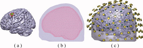
(a) An example of CCD source model with examples for simulated small extended cortical source (green area) and large extended cortical source (green and red areas). (b) An example of a BE volume conductor model consisting of the scalp (light blue), the skull (red), and the brain (gray). (c) Co‐registration between EEG electrodes (green), MEG sensors (yellow), BE model, and CCD model. [Color figure can be viewed in the online issue, which is available at wileyonlinelibrary.com.]

EEG electrode locations and MEG sensor locations and orientations were adopted from the realistic EEG and MEG systems. In order to simulate similar spatial coverage of EEG sensors as that of MEG, a subset of 120 EEG channels were selected from a realistic 128‐electrode EGI system (Electrical Geodesics, Inc., Eugene, OR) by removing some electrodes on face. EEG channels were also evenly downsampled in space to 63 and 30 locations to simulate different number of electrodes covering similar area of sampling space. For MEG, there were 151 MEG sensors from a 151 channel CTF Omega system, and the downsampled configuration of 100 and 47 channels were similarly generated as in the EEG. We also studied the effects of various combinations of EEG electrode and MEG sensor configurations. Both EEG electrode and MEG sensor locations are illustrated in Figure 1c, overlaid with BE and CCD models.

To formulate the forward problem, the vector is used to represent N elemental dipole moments defined on the CCD model. Vectors and denote potentials and magnetic fields at M _v EEG electrodes and M _b MEG sensors, respectively. is the gain matrix (M _v × N) calculated by BEM for electrical potentials, whereas is the gain matrix (M _b × N) for magnetic fields. Both and denote background and measurement noises in EEG and MEG. Then the forward problem can be expressed in the following vector notation:

(1)

SNR Transformation

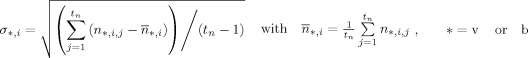
Since EEG and MEG data have different measures (i.e., units), to combine them, they have to be converted to a common basis. We utilized the SNR transformation concept proposed in previous studies [Fucks et al., 1998; Greenblatt, 1995], which converts all channel data into the SNR domain, and applies the sESI method according to the statistical significance of data as indicated by the SNR. Specifically, a channel‐wise SNR transformation was utilized by estimating the standard deviations σ of noise from each channel for both EEG and MEG.

(2)

where i indicates the ith channel, j indicates the time point, and t _n is the number of time points in noise. In the analysis of experimental data, noise data can be selected from recordings considered as signal free (e.g., pre‐stimulus data). The SNR transformation can thus be performed by normalizing EEG/MEG signals to their individual standard deviation of noise, yielding unit‐free measures for both electric and magnetic modalities, using the following equation:

(3)

Note that the SNR transformation alters the relationship between electrical/magnetic fields and the dipole moments. The EEG/MEG gain matrices need to be changed accordingly to avoid inconsistency since channels (especially EEG/MEG channels) are normalized differently.

(4)

Each row of gain matrices is normalized by the individual standard deviation of noise from the corresponding channel. Then, the columns of the MEG gain matrix are appended to the corresponding columns of the EEG gain matrix. The combined forward problem can thus be expressed as follows:

(5)

where A is the combined gain matrix . Note that noise from EEG/MEG recordings is also modified and their variances become unity. In studies using EEG/MEG data alone, the channel‐wise SNR transformation was also performed to make it consistent with combined EEG and MEG analysis and also compensate for different noise levels from different channels.

Sparse Representation of Extended Cortical Sources

It has been suggested that detectable EEG/MEG sources primarily consist of synchronized intracellular currents flowing through pyramidal neurons, which cover extents at least 40 mm² [Chapman et al., 1984], or possibly even much larger. This indicates that an extended cortical patch, consisting of many elemental dipoles distributed over the convoluted cortical surface, is a realistic model for EEG/MEG sources. Many previous L1‐norm regularized imaging approaches [Huang et al., 2006; Uutela et al., 1999; Wagner et al., 1998] directly penalized the L1‐norm of solution vector . Since elemental dipoles within a cortical patch are closely located, projections of their activity on electrodes/sensors share largely overlapping patterns. Penalties on the L1‐norm of solution vectors tend to minimize the L1‐norm by accumulating elemental dipole moments onto one (or few) location(s) with diminished extents. The enforcement of such sparseness in the source domain thus produces over‐focused solutions [Ding and He, 2008]. In VB‐SCCD, however, we proposed to penalize the variation vector, which is in a transformed domain of the source vector [Ding, 2009], with the L1‐norm. The variation vector represents the variation map of cortical source distributions (or current density maps), which characterize boundaries between active (i.e., source) and inactive cortical regions (i.e., non‐source) as the main sparse feature (or the sparseness). This new sparse feature obviously does not enforce over‐focused solutions and has been shown to better represent extended cortical sources [Ding, 2009]. We proposed an operator V to obtain variation maps:

(6)

where V is a P × N matrix and P is the total number of edges from triangular elements. Each row of V corresponds to an edge i and only two elements (which share the same edge i) within the row have non‐zero values, i.e., 1 and −1.

Variation‐Based Sparse Cortical Current Density Algorithm

By minimizing the L1‐norm of , the regularization scheme in VB‐SCCD is formed as:

(7)

Each element in this variation vector represents a coefficient defined on a triangular edge and its value indicates the current density difference between two triangular elements which share the same edge. If the cortical current density within each individual active cortical source is close to uniform or can be approximated with uniform distributions, non‐zero coefficients are expected to exist mainly on boundaries (the sparse feature) and expected to be identified by minimizing the L1‐norm of this variation vector. The second term in Eq. (7) is the data term, which calculates the error between recordings and predicted values from the forward model [i.e., Eq. (5)]. This error will only be allowed to be less than a parameter, β, obtained based on the noise level, which guarantees the consistency between recordings and reconstructed results. The parameter β, known as the regularization parameter, is estimated using the discrepancy principle [Morozov, 1966]. We choose it to be high enough so that the probability of , where , is small. When we assume Gaussian white noise, follows a Chi‐square distribution, χ_m with M degrees of freedom, i.e., . Because of the SNR transformation, σ₂ for both EEG and MEG signals have become unity and thus . In practice, the upper bound of , i.e. β, is selected such that the confidence interval [0, β] integrates to a 0.99 probability [Ding and He, 2008]. The variance σ² for real data was estimated using the method discussed in the section of SNR transformation.

Solver: Second‐Order Cone Programming

The optimization problem stated in Eq. (7) is a convex optimization problem, which can be solved efficiently with globally optimal solutions. It was solved using the second order cone programming (SOCP) technique [Nemirovski and Ben Tal, 2001], which utilizes the efficient globally convergent solver known as the Interior Point Methods (IPM). The method has been implemented in the MATLAB package SeDuMi [Sturm, 2001]. In order to solve them, these problems should be formulated into the framework of SOCP (details for this approach can be found in our previous study [Ding, 2009]).

Monte Carlo Simulation

It is well known that the accuracy of inverse solutions is highly dependent on the location of source [Fuchs et al., 1998; Liu et al., 1998] due to different sensitivities of EEG/MEG to sources from different locations with different orientations and depths. Simulations with a large number of randomly sampled source locations [Liu et al., 2002] has been suggested to better represent realistic conditions in which electrical activity can occur in the brain. In our simulation, cortical sources were generated by selecting a seed triangular element on the cortical mesh and gradually growing into patches by iteratively adding neighboring elements. The dipole moment on each triangle was computed as the multiplication of the individual triangular area and the dipole moment density (i.e., 100 pAm/mm²). Different brain activity was simulated with a different number of cortical sources (i.e., 1, 2, 5, and 10 sources). The locations of these sources were randomly selected. The cortical extents of these sources were simulated with small sizes (2.33 ± 0.34 cm²) and large sizes (7.83 ± 1.11 cm²; Fig. 1a). We further investigated the effects of using different numbers of electrodes/sensors and different signal modalities (i.e., EEG alone, MEG alone, and EEG+MEG). For each condition (such as, different number of sources, different number of electrodes/sensors, and different modalities), we repeated the simulation 200 times to cover most parts of the brain during the random sampling procedure. Noiseless EEG/MEG signals generated by individual elemental dipoles in a cortical source were calculated using BEM and were then superposed to obtain the surface fields of the cortical source. If there were multiple sources in one simulation, surface fields from these sources were superposed again. Simulated EEG/MEG data were then contaminated by real noise recorded from a subject in resting conditions and calibrated to a 10 dB SNR.

We used the metrics, i.e., the receiver operating characteristic (ROC) curve and the area under the ROC curve (AUC) from detection theory [Grova et al., 2006] to assess the performance of VB‐SCCD in simulation data. Cortical current distributions reconstructed from simulated data can be thresholded (namely α) to determine active and inactive cortical regions that are compared with simulated source distributions. An active element in the simulated map is regarded as a true positive (TP) if it is an active element in the reconstructed map thresholded at α. Otherwise, this element is a false negative (FN). An inactive element in the simulated map is regarded as a false positive (FP) if it is an active element in the reconstructed map thresholded at α. Otherwise, this element is a true negative (TN). Specificity and sensitivity are then defined as:

(8)

ROC curves can be obtained by plotting against at different thresholds. The AUC metric is calculated as the area under ROC curves. High AUC values indicate both high sensitivity and high specificity in detecting extended cortical sources. To obtain an unbiased estimation of the AUC metric, a similar number of simulated active and inactive elements should be provided, which is obviously not the case in our simulation study. We used a method reported in Grova et al. [2006] to obtain less biased AUC values. Briefly, a set of simulated inactive elements, which has the same number as simulated active elements, was randomly selected from the total number of inactive elements to compute the AUC. The random selection process was repeated 50 times to reduce the bias caused by a specific set selected in one realization. Furthermore, since it is well known that spurious sources from most inverse solutions usually happen in the neighboring elements around simulated active elements, we thus split the inactive elements into two groups, i.e., elements within the 10th neighborhood (in terms of triangular elements) of simulated active elements, and elements beyond the 10th neighborhood. AUC values were computed separately for inactive elements from these two groups using the random process described above and then averaged [see details in Ding, 2009]. Although most previous studies reporting ROC metrics for EEG/MEG allow certain source localization bias within a pre‐defined acceptable distance of active sources [Darvas et al., 2004; Grova et al., 2006], in the present study, we used the “hard” AUC metric that allows no such bias. To achieve high AUC values, estimations of locations and cortical extents of sources must be accurate.

Experimental Protocol and Data Analysis

To evaluate the performance of the proposed approach with empirical data, we performed an analysis of the face processing event‐related potentials (ERPs) and fields (ERFs) data obtained from the EEG and MEG, respectively. Details of the experimental paradigm as well as the full dataset can be found at http://www.fil.ion.ac.ik/spm/data/mmfaces.html. Briefly, EEG and MEG data were recorded in a subject performing a face perception task [Henson et al., 2003]. The subject made symmetry judgments on faces and scrambled faces. Stimuli of faces and scrambled faces were presented every 3.6 s and each stimulus lasted 0.6 s. EEG data were acquired on a 128‐channel ActiveTwo system, sampled at 2,048 Hz, whereas MEG data were sampled at 625 Hz from a 151‐channel CTF Omega system. Both EEG and MEG data were subsequently downsampled to 200 Hz and interpolated to align EEG and MEG samples in the time domain. Epochs were created from −200 ms to 600 ms for both EEG and MEG. These epochs were then detrended and examined for artifacts. The epochs were averaged according to the two trial types: faces (F) and scrambled faces (S), to produce type‐specific ERPs and ERFs. Note that face stimuli included both familiar and unfamiliar faces, and both were combined to create event‐related data.

The subject's T1‐weighted MRI was obtained from a 1.5T Siemens Sonata via an MDEFT sequence with resolution 1 × 1 × 1 mm³ voxels, using a whole body coil for RF transmission and an 8‐element phased array head coil for signal reception. The CCD source model and BEM volume conductor were built using BrainSuite software. The cortical surface was triangulated into a high‐resolution mesh with 63,820 triangles (triangle area: 2.78 ± 2.11 mm²; Fig. 9). The subject's head shape (including nasion, left, and right preauricular fiducial points) was digitized (Polhemus, Inc., Colchester, VT). In EEG recordings, electrode locations were also digitized. We first co‐registered the EEG, MEG, and BEM mesh using a rigid transformation based on the location of the three fiducial points. We then refined this registration using a surface‐fitting algorithm [Towle et al., 2003] via minimizing the fitting errors between the BEM meshes and digitized electrode positions for EEG, and the digitized head shape for MEG.

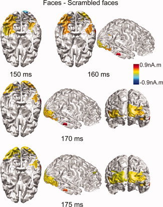
Figure 9.

Dynamic patterns of source reconstructions within P100/M100 and P170/M170 components from a face recognition task. (a) An EEG waveform from one channel (red electrode shown registered with the head) and a MEG waveform from one channel (green sensor), both of which show the maximal difference between faces and scrambled faces. (b) Cortical current density maps reconstructed within P100/M100. (c) Cortical current density maps reconstructed within P170/M170. [Color figure can be viewed in the online issue, which is available at wileyonlinelibrary.com.]

RESULTS

Reconstruction of Multiple Cortical Sources

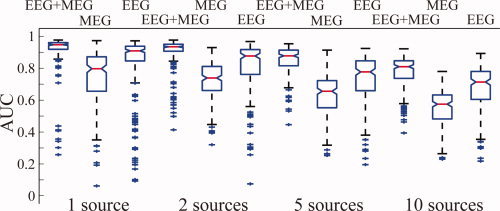
Figure 2 shows the AUC values for simulations under different conditions, such as the number of sources, number of electrodes, and EEG/MEG modalities from simulated cortical sources of small sizes. We first investigated the performance of the integrative approach in reconstructing multiple cortical sources (i.e., 1, 2, 5, and 10). As indicated by the general trend in Figure 2, when the number of sources increased, the AUC metric decreased for EEG, MEG, and EEG+MEG, and for different number of channels. For example, when examining the MEG+EEG (120+151) conditions from one to ten sources, we can observe that their median AUC values slowly decrease from above 0.95 to slightly higher than 0.8. However, it is worthwhile to note that the overall reconstruction accuracy in these conditions is considered high since most of AUC values are higher than 0.8 [Grova et al., 2006], even when there are ten simultaneously activated and randomly located sources. This observation can be generalized to other EEG+MEG conditions (i.e., first nine columns in Fig. 2). Generally, the median AUCs in simulations using up to five sources are higher than 0.8, and in the conditions of 10 sources, they are around 0.8 (depending on the number of EEG and MEG channels used). The performance of the integrative approach is also reflected in variations of 200 random repeats. We used the difference between the 25th and 75th percentiles of data (i.e., the length of the boxes in Whisker plots) as a measure of variation. From one to ten sources, we observed that this measure increased for all EEG+MEG conditions no matter how many channels were used. This suggests that performance decreases as the number of sources increases, while the general performance is reasonably good as indicated by the median AUCs. However, this measure shows an opposite general trend in the EEG or MEG alone data, where its values decrease as the number of sources increase, and are found to be considerably larger than those from EEG+MEG. This phenomenon can be explained by large sensitivity variations of EEG or MEG in different source configurations, which will be discussed in details below.

Figure 2.

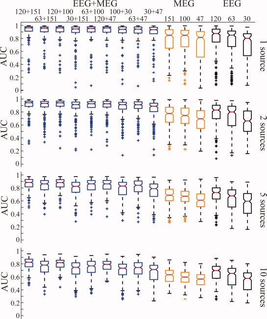
Whisker plots of AUC metric values for VB‐SCCD using EEG (black), MEG (orange), and EEG+MEG (blue) with different numbers of channels (from right to left: 30, 63, and 120 for EEG; 47, 100, and 151 for MEG; and 30+47, 63+47, 100+30, 120+47, 63+100, 30+151, 120+100, 63+151, and 120+151 for EEG+MEG) and with different source configurations (1, 2, 5, and 10 sources) from simulated sources of smaller sizes. [Color figure can be viewed in the online issue, which is available at wileyonlinelibrary.com.]

Although Whisker plots of AUC values provide an overall picture of performance of the integrative approach, Figures 3 (for 1, 2, and 10 sources) and 4b (for 5 sources) allow us to directly visualize the reconstructed extended cortical sources from the best five examples in reference to corresponding simulated ones. These reconstructed distributions were uniformly thresholded at 20% of their own global maximal values. When there are only a few simulated sources (i.e., 1 or 2), the reconstructed distributions are almost exactly recovered in terms of location and spatial extent (Fig. 3a,b). When the number of sources increases to five, all cortical sources can still be resolved, and their localizations are accurate. For example, in the case of #5 (Fig. 4b), all five reconstructed cortical sources on the same hemisphere are well reconstructed, and, in the case of #3, four sources (marked by a, c, d, and e) within a close neighborhood are well resolved. At the same time, these sources start to exhibit larger extents than simulated ones under 20% thresholding. Notably, when the number of sources to be reconstructed is ten (Fig. 3c), the reconstructed cortical sources have consistent distributions and many closely located sources are still able to be resolved, while more cortical sources have enlarged spatial extents. Since the chance for randomly selected sources being close becomes higher when the number of sources increases, some of the closely located sources are fused. In summary, these examples demonstrate the remarkable resolvability of the integrative approach in localizing multiple sources (up to 10). Of course, the reduced performance for an increased number of sources is also suggested in these examples as shown in Whisker plots of AUC values.

Figure 3.

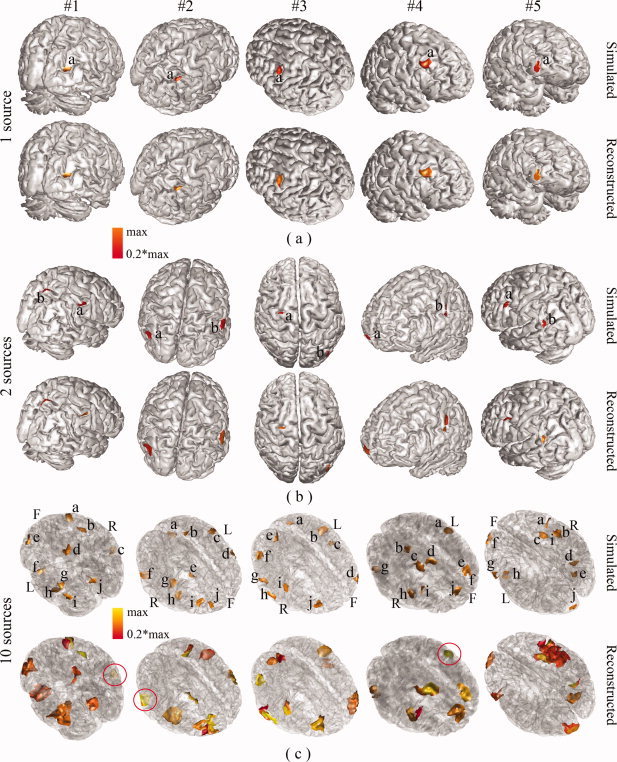
Illustration of the five best reconstructions (from #1 to #5) from different source configuration: (a) 1 source; (b) 2 sources; and (c) 10 sources. First rows: simulated cortical maps with each source marked by a letter; second row: reconstructed cortical maps by VB‐SCCD. One or two views were used to show all randomly generated sources. When two views were not enough, transparent cortical models were used and capital letters L (left), R (right), and F (front) were used to mark the orientation of cortical models. For illustration purposes, the simulated sources were marked by letters and some reconstructed sources were circled. [Color figure can be viewed in the online issue, which is available at wileyonlinelibrary.com.]

Figure 4.

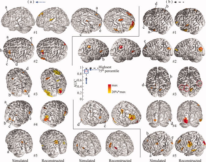
Illustration of five reconstructions with five simulated sources at different percentiles of AUC values from 200 repeats: (a) highest or 100th percentile; (b) 75th percentile. Same display conventions as in Figure 3. [Color figure can be viewed in the online issue, which is available at wileyonlinelibrary.com.]

Reconstructed Cortical Distributions at Different Levels of Performance

In the above section, we discussed the performance of the integrative approach in conditions with different number of sources using the best five examples. Here, we show examples of reconstructed source distributions at different levels of performance as indexed by AUC values from simulations of five sources as a representative case for multiple sources. We selected five examples at each quartile of AUC values [i.e., the 100th (highest), 75th, 50th, 25th, and or 0th (lowest percentile). These are illustrated in Figures 4 and 5.

Figure 5.

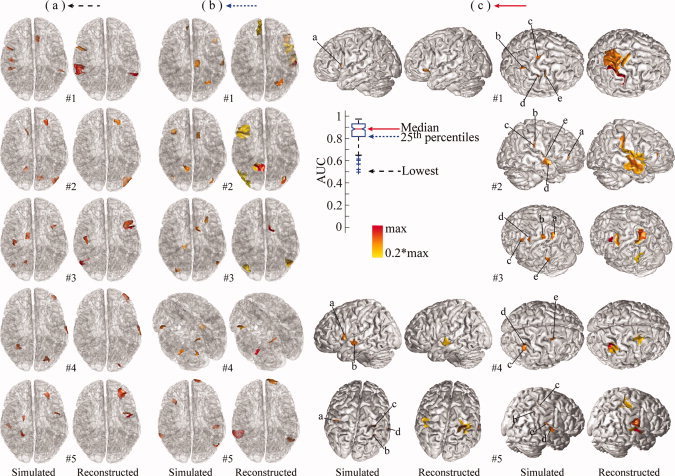
Illustration of five reconstructions with five simulated sources at different percentiles of AUC values from 200 repeats (continue): (a) median or 50th percentile; (b) 25th percentile; (c) Lowest or 0th percentile. Same display conventions as in Figure 3. [Color figure can be viewed in the online issue, which is available at wileyonlinelibrary.com.]

Generally, the pattern of reconstruction accuracy from the best (Fig. 4b) to the worst (Fig. 5a) is consistent with the pattern of the AUC metric. The variation of reconstruction accuracy is mainly caused by the locations of simulated sources since other influential factors, such as number of sources, extent, and SNR are the same or very similar. In order to further discuss the location‐dependent performance of the proposed integrative approach, we examined three types of distortions in reconstructed source distributions, which affect the AUC value: enlarged extent, fused source distribution, and missing sources. Both enlarged extent and fused distribution have been observed in Figure 3 and they are related since closely located sources with enlarged extent tend to fuse together. It is obvious that these three types of distortions are present at different AUC values. The phenomenon of enlarged spatial extent starts to appear in examples with the highest AUC values (Fig. 4b), such as cases #4 and #5, and becomes significant in examples at the 75th percentile (Fig. 4a). The phenomenon of fused distribution starts from the 75th percentile (Fig. 4a), as in case #4, and appears more at the 50th and 25th percentiles (Fig. 5b,c). The missing source mainly appears in the 25th percentile and lowest portion of AUC values. Among them, the missing source represents the most significant problem in source identification. While the problem of enlarged extent leads to smooth reconstructions, fused distributions occur when reconstructions are further smoothed, which leads to reduced spatial resolvability of sources. It is also worthwhile to note that these three distortions affect the AUC metric differently. Both the enlarged extent and fused distribution problems have increased FP values, which decrease the specificity of detection and lead to low AUC values. On the other hand, missing sources increase FN values, which decrease the sensitivity of detection and lead to low AUC values.

In addition, it is interesting to note that both enlarged extent and fused distribution problems are not as evident as the missing source problem at the lowest and 25th percentile of AUC values. This indicates that the missing source problem biases the AUC metric more significantly. We observed that most missing sources are located either on median walls of both hemispheres or within deep structures, where both EEG and MEG have low sensitivity to detect them. It is also important to note that the performance in reconstructing other cortical sources is not obviously influenced by the existence of these missing sources and their unaccounted residual fields (due to the fact that these sources are not reconstructed; Fig. 5a,b).

Performance of EEG, MEG, and EEG+MEG

Figure 2 also illustrates the large difference observed between EEG alone, MEG alone, and EEG+MEG. Any combination of EEG and MEG has better performance (i.e., higher median AUC values) than EEG or MEG alone in all conditions (i.e., from 1 to 10 sources). For example, the combination of low‐density (30 channels) EEG and low‐density (47 channels) MEG (total 77 channels) has better AUC values than high‐density EEG alone (120 channels) or high‐density MEG alone (151 channels). This effect was statistically significant across most conditions with different numbers of sources (p < 0.05). This indicates that the complementary nature of EEG and MEG improves the source reconstruction performance much more significantly than simply adding more EEG electrodes or MEG sensors. This observation is also collaboratively supported by relatively smaller variations (as indicated by the length of box in Whisker plots) in EEG+MEG than EEG or MEG alone. The large variations in EEG or MEG alone are due to largely varying sensitivity of EEG or MEG to differently configured cortical sources (i.e., from different locations). These large variations cannot be significantly reduced with increased number of channels in a single modality since it does not significantly enhance the sensitivity profile. Meanwhile, since EEG and MEG have different sensitivity profiles for differently configured sources, the variation dependent on locations can be reduced by combining them.

As indicated by the AUC data, there is no obvious difference between the performance of EEG and MEG alone. EEG performs better in terms of AUC than high‐density MEG measurements (120 EEG channels and 151 MEG channels), whereas MEG performs better in low density (47 channels) than EEG (30 channels). However, such differences are not as large as the difference between EEG+MEG and EEG or MEG alone. Both EEG and MEG have large variations of AUC values in simulations of one source and relatively low variations of AUC values in simulations of five or ten sources. Since the performance of EEG or MEG alone is highly dependent on location, some sources are relatively more difficult to be reconstructed than others. When such a source occurs in simulations of only one source, it influences the entire distribution and leads to extremely low AUC values (thus large variation in AUC values). However, when it occurs in simulations of five sources or ten sources, it only disturbs ∼ 20% or 10% of distributions and does not produce extremely low AUC values (thus relatively small variation in AUC values).

Figure 6 illustrates the difference of EEG, MEG, and EEG+MEG in two examples from simulations of five sources. It is obvious that the improvement of EEG+MEG in localizing extended cortical sources and reconstructing their spatial extents is significant compared to EEG or MEG alone. For example, in Figure 6a, the result from EEG+MEG resolves two closely located sources (marked as a and b) in the left front area which could not be separated using EEG. Furthermore, the reconstructed distributions of five sources from EEG+MEG are much more consistent with simulated distributions compared to EEG. As compared with MEG, EEG+MEG identifies missing sources in MEG (two in Fig. 6a, marked as c and e, and one in Fig. 6b, marked as b). It is also notable that EEG+MEG can significantly correct the localization bias. For example, in Figure 6b all five sources identified by EEG are significantly biased from their simulated sites (although still in the neighborhoods) and two sources identified by MEG (marked as c and d) are also shifted, whereas the same five sources are all correctly located using EEG+MEG. The largest distortion in the distribution from EEG+MEG, in the second example, is that it indicates an enlarged spatial extent of source b located in the deep structure. However, the same source is either missing in MEG or significantly biased in EEG.

Figure 6.

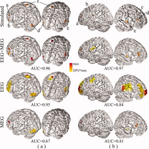
Comparison between EEG (120 channels), MEG (151 channels), and EEG+MEG (120+151 channels) in reconstructing five sources. (a) The 1st example; (b) the 2nd example. Same display conventions as in Figure 3. [Color figure can be viewed in the online issue, which is available at wileyonlinelibrary.com.]

Number of Electrodes/Sensors

The influence of the number of electrodes/sensors on the performance of the integrative approach, as indicated by the AUC metric (Fig. 2), is not as significant as the influence of modality. In the single modality analysis (i.e., EEG or MEG), the AUC metric decreased as the number of electrodes/sensors decreased, and these reductions become statistically significant between high‐density (>100 channels) recordings and low‐density (<50 channels) recordings. This general trend is common and similar for both EEG and MEG and for all simulations with different numbers of sources. While the performance for combined MEG and EEG data is better when more electrodes and sensors are used, this influence is not as significant as in a single data modality, and the resulted differences are not statistically significant in most cases. Although such differences are not quite visible in simulations with few numbers of sources (i.e., 1 and 2), high‐density data showed significantly better performance as the number of simulated sources increased (i.e., 5 and 10).

Size of Cortical Sources

Figure 7 shows the AUC values for simulated cortical sources of larger sizes. Only results from EEG+MEG (120+151 channels), EEG (120 channels), and MEG (151 channels) for one, two, five, and ten sources are presented here, whereas other data share the similar pattern. Compared to the results from the simulated cortical sources of smaller sizes shown in Figure 2, there were no significant changes in AUC values for both EEG+MEG and EEG alone across conditions with different numbers of sources. We observed a significant decrease of AUC values for MEG alone in all conditions. Such a reduction was probably caused by the increased radial components in simulated sources when their spatial sizes over the cortical surface increased. Since MEG is insensitive to radial sources [Baule and McFee, 1965], the radial components in extended cortical sources might be underestimated and thus impact the value of AUC metric.

Figure 7.

Whisker plots of AUC metric values for VB‐SCCD using EEG (120 channels), MEG (151 channels), and EEG+MEG (120+151 channels) with different source configurations (1, 2, 5, and 10 sources) from simulated sources of larger sizes. [Color figure can be viewed in the online issue, which is available at wileyonlinelibrary.com.]

Comparison of External EEG/MEG Recordings and Reconstructed Cortical Maps

Figure 8 illustrates four examples of external EEG (120 channels) and MEG (151 channels) recordings together with their reconstructed cortical maps (un‐thresholded) with one, two, five, and ten sources. These EEG and MEG maps generally have limited spatial resolution due to the so‐called volume conductor effect. Moreover, the underlying cortical generators behind them are not well defined spatially since both EEG and MEG have limited spatial penetration, and their distributions depend on the orientations of current flows. Additionally, cortically reconstructed source distribution maps gain spatial penetration, which avoids the complications from the volume conductor effect, and further enhances the spatial resolution. In the cases with few sources (i.e., 1 and 2; Fig. 8a,b), EEG and MEG are able to provide non‐overlapped (or not significantly overlapped) field maps (if sources are not too close to each other in cases with more than one source), even though the signals have smooth spatial distributions. It is thus possible to use EEG and MEG signals directly when assessing underlying activity and the major function of ESI (or sESI) is to accurately locate the activity on corresponding anatomic structures and precisely estimate their spatial extents. In the cases with more sources (i.e., 5 and 10; Fig. 8c,d), both EEG and MEG field maps are significantly overlapped (either enhanced or canceled) and it is thus difficult or almost impossible to perform direct interpretations. VB‐SCCD thus performs spatial de‐convolutions on EEG and MEG maps when reconstructing source locations and extents. While the mathematical problem becomes more challenging, the gain by performing sESI increases more significantly. Examples in Figure 8c,d demonstrate how much spatial information can be gained by reconstructing sources from surface EEG and MEG.

Figure 8.

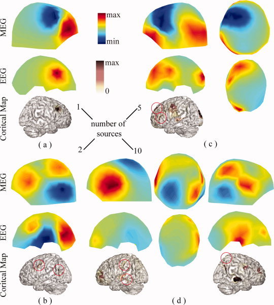
Illustrations of spatial localization and resolvability of sources at different levels via comparing scalp EEG (120 channels), scalp MEG (151 channels), and cortical maps reconstructed from EEG+MEG (120+151 channels). (a) One source; (b) two sources; (c) five sources; and (d) 10 sources. [Color figure can be viewed in the online issue, which is available at wileyonlinelibrary.com.]

Cortical Sources for Face Perception and Recognition

Source imaging results from multiple time points for face perception and recognition are illustrated in Figures 9, 10, 11, which used the same pseudo‐color representations to make brain activations at different time points comparable. Each individual cortical map was uniformly thresholded at 30% of its own maximal value. The difference maps in Figure 10 were created by subtracting source maps for scrambled faces from those for faces and then thresholded at 30%. Figure 9a shows the cortical sources from EEG+MEG for P100/M100 components in both conditions of faces and scrambled faces. Large activities are shown in the primary and associated visual cortices. The spatial distributions of these cortical sources and their temporal dynamics (i.e., their changing spatial patterns within multiple time points) are consistent between faces and scrambled faces, which indicates no obvious difference of brain computations in processing both stimuli during the time window for P100/M100.

Figure 10.

Difference maps obtained via subtracting cortical current density maps of scrambled faces from maps of faces within P100/M100. [Color figure can be viewed in the online issue, which is available at wileyonlinelibrary.com.]

Figure 11.

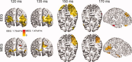
Comparison between EEG, MEG, and EEG+MEG (shown in Fig. 8) in reconstructing sources within both P100/M100 and P170/M170 components of faces. [Color figure can be viewed in the online issue, which is available at wileyonlinelibrary.com.]

The difference between faces and scrambled faces has been reported in EEG/MEG at the N170/M170 component and has also been studied with fMRI data using the same protocol from the research group [Henson et al., 2003] who shared the EEG/MEG dataset utilized in our present study. We shall discuss our findings using the proposed integrative analysis approach with reference to their findings from the fMRI data [Henson et al., 2003]. During N170/M170, it was observed that bilateral fusiform (i.e., 150–160 ms) and lateral ventral occipital regions (i.e., 160–175 ms) were more active for faces compared to scrambled faces (Fig. 9c). A similar difference was observed in fMRI activation maps [Fig. 5A and Table 3 in Henson et al., 2003]. Furthermore, posterior occipital regions, as indicated in the difference maps (Fig. 10), were more active for scrambled faces during the early phase of N170/M170 (e.g., 150 ms) and P100/M100 (data not shown here), and became less active during the late phase of N170/M170 (e.g., 170–175 ms). The same area appeared more active in the scrambled faces than in faces, as suggested by fMRI data [Fig. 5A and Table 3 in Henson et al., 2003], which reflected summed brain activity within the entire studied time window (including N170/M170 and P100/M100) due to the low temporal resolution of the hemodynamic response. Other notable areas, which are more active for normal faces, included the right superior temporal sulcus (STS; e.g., 160 ms marked by a circle) and right lateral temporal gyrus, which also happened to be consistent with the fMRI data [Fig. 5A and Table 3 in Henson et al., 2003].

Brain areas showing significant activity within the frontal lobe to face stimuli included the medial superior frontal gyrus, the orbital part of inferior frontal gyrus, and the medial orbitofrontal gyrus (e.g., 175 ms marked by a circle; Fig. 9c). These observations were in line with the fMRI data [Fig. 6A and Table 4 in Henson et al., 2003]. The difference in activation between familiar faces and unfamiliar faces suggests that these regions are involved in face recognition. However, EEG/MEG trials for both familiar and unfamiliar faces were averaged during the creation of ERP/ERF and thus these activities reflected the overall brain responses to both conditions. Similar activity in these brain areas was also observed for scrambled face stimuli, which appeared to be more localized before 160 ms and much more spread from 170 ms. At the time points around 170 ms (or 175 ms), EEG/MEG signals were observed to be much smaller for scrambled faces than those for faces and resulted in low SNRs, which might be the reason why less reliable and smooth reconstructions were produced. In Figure 10, the difference between faces and scrambled faces were found in the occipital and temporal cortices but could not be identified in the frontal cortex. This might be caused by averaging brain responses to familiar and unfamiliar faces which smears the contrast. However, sources within the frontal cortex for face stimuli are much more localized than responses for scrambled faces during N170/M170 (especially its late phase) due to the higher SNR.

Figure 11 illustrates the EEG and MEG results for faces during both P100/M100 and N170/M170, and compares the results for the combined EEG+MEG shown in Figure 9. Sources reconstructed from EEG or MEG are generally consistent with those from EEG+MEG, but with degradations. Bilateral fusiform activations appear unilateral in both EEG alone and MEG alone, which is similar to source localization results from another study using the same MEG dataset [Henson et al., 2005]. Specifically, fusiform activations from EEG are only reconstructed at one time point (i.e., 150 ms). Meanwhile, EEG has much better accuracy in reconstructing sources within the frontal cortex (e.g., 170 ms). MEG has better resolutions in occipital and temporal cortices while it totally loses sources within the frontal cortex. Furthermore, sources reconstructed from MEG seem much more localized compared with sources reconstructed from EEG (e.g., 120 ms and 135 ms), which is also observed in simulations (Fig. 6).

DISCUSSION

In the present study, we demonstrated that a novel sparse ESI technology (i.e., VB‐SCCD) is able to reconstruct complicated brain activations (up to 10 simultaneous activations as in current simulations) via integrating EEG and MEG data. Reconstructed cortical brain activations from both simulations and experimental data provided precise source localizations as well as accurate estimation of source spatial extents. The performance of VB‐SCCD is significantly improved with combined EEG and MEG as compared with EEG or MEG alone. We further demonstrated that, with VB‐SCCD and combined EEG and MEG, it is promising to noninvasively estimate the spatiotemporal dynamics of complex brain activations in real data (i.e., a face recognition task).

In our simulations, a Monte Carlo protocol was implemented with the number of sources up to 10, which is one of the few EEG/MEG studies, to our knowledge, using randomly generated multiple source (more than five) schemes [Liu et al., 1998]. We evaluated the simulation results with the AUC metric [Grova et al., 2006] (Fig. 2). In the design of the AUC metric, we implemented a random selection process by balancing the sizes of active and inactive elements to reduce the bias on the calculation of AUC metric due to large number of inactive elements. We also adopted a strategy of computing AUC values by splitting inactive elements into two groups, which are either close to or far away from simulated sources, in order to correct the underestimation of false positives due to the non‐uniform distributions of spurious sources [Grova et al., 2006]. As a result, the adopted AUC metric is sensitive to both localization biases and estimation errors of source extents [Ding, 2009]. Meanwhile, the evaluation metric (i.e., AUC) and its statistics (i.e., Whisker plots of AUC) are not straightforward in revealing how a real inverse solution looks like. We thus further accessed the simulation results by directly inspecting reconstructed source maps (Figs. 3, 4, 5). Overall, our simulation data suggest that the VB‐SCCD technique is capable of reconstructing complicated cortical activation maps (i.e., of multiple randomly located sources). The reconstructed cortical maps are accurate in terms of localization and extent estimation with few numbers of sources (i.e., 1 or 2). In conditions with five or ten sources, reconstructed sources are accurate in terms of localization in most cases whereas their extent estimations are degraded because of smeared spatial distributions or multiple fused activities. In some extreme cases, there are missing sources (Fig. 5). The present results also suggest the robustness of VB‐SCCD in reconstructing extended cortical sources with different spatial sizes (Fig. 7). Generally, our data indicate that VB‐SCCD using combined EEG and MEG is able to significantly enhance the spatial resolvability on cortical sources when it is compared with surface EEG and MEG (Fig. 8), especially in cases with multiple sources (five sources in Fig. 8c and ten sources in Fig. 8d).

Our present study also investigated the performance of VB‐SCCD using experimentally recorded EEG and MEG data from a face recognition task [Henson et al., 2003]. We conducted source analysis using ERP and ERF data during both P100/M100 and N170/M170 components. The cortical source maps from faces and scrambled faces during P100/M100 are almost identical, whereas the most significant difference between cortical maps for faces and scrambled faces appears during N170/M170 (Fig. 10). This observation is consistent with our physiological understanding that the same brain process should occur during P100/M100 since both faces and scrambled faces are visual stimuli. However, different brain processes are expected to be observed since face stimulus is supposed to provoke the brain response for face recognition while scrambled faces are not. Within N170/M170, an extensive brain network, involving bilateral fusiform, posterior occipital regions, STS, right lateral temporal gyrus, medial superior frontal gyrus, and inferior and medial orbitofrontal gyri, was recovered and its spatiotemporal dynamics were reconstructed (Fig. 9). We compared our findings with findings from an fMRI study using the same protocol [Henson et al., 2003] and indicated that all observations were consistent and a complete cortical network underlying face recognition as reconstructed by fMRI can be similarly recovered by VB‐SCCD with the combined EEG and MEG, which has much higher temporal resolutions to further resolve the temporal sequence of activation incidence. Furthermore, our observations were also consistent with findings related to face recognition from other studies [Hasselmo et al., 1989; Haxby et al., 2000; Scalaidhe et al., 1999]. For example, bilateral activations of fusiform areas have been identified in association with face‐processing [Haxby et al., 2000] and have been similarly recovered by another study using same EEG dataset [Friston et al., 2008]. Another example is that the neurons in STS are suspected of being sensitive to face expression [Hasselmo et al., 1989]. At each instant in time, reconstructions of multiple brain activations distributed over multiple cortices (e.g., eight spatially distinct activations at 160 ms from faces stimulus, Fig. 9) demonstrate the excellent capability of the proposed novel integrative approach in investigating complicated brain processes. Figures 9 and 10 further indicate the stable temporal dynamic patterns and consistent temporal dynamic difference patterns between faces and scrambled faces, respectively, revealed by the source analysis.

The novel L1‐norm regularization scheme proposed in sESI (e.g., VB‐SCCD) addresses the fundamental mathematical challenges of EEG/MEG inverse problems, i.e., the non‐uniqueness, in a new perspective. According to information theory [Candes and Tao, 2005], the L1‐norm regularized optimization problems can be solved with exact solutions if the number of sparseness (i.e., the number of non‐zero coefficients if in a transformed domain) is small enough compared with the number of measurements. From this new perspective, the severity of underdetermined problem of EEG/MEG inverse problems is not determined by the ratio between the number of sources and the number of measurements (e.g., 50,000:200), but by the ratio between the number of sparseness and the number of measurements. In VB‐SCCD, the sparse feature is characterized in the variation domain and its effectiveness in reconstructing extended cortical sources has been studied with EEG [Ding, 2009] and MEG data [Ding et al., 2010]. In the current study, we increased the number of measurements by changing the number of electrodes/sensors, and by using single modality data (EEG or MEG) or multiple modality data (EEG+MEG). Our current results suggest that data from multiple imaging modalities (i.e., EEG and MEG) are more effective in improving the performance of VB‐SCCD than increasing number of channels from a single modality. This is due to the fact that EEG or MEG recordings are structurally constrained to the head surface and their measurements can be highly correlated (i.e., interdependent). Meanwhile, the significant improvement of performance in VB‐SCCD with the combined EEG and MEG is due to the fact that EEG and MEG have different sensitivity profiles to brain sources, and thus provide more independent information. This is consistent with the CS theory that orthogonal measurements are needed to achieve exact solutions in L1‐norm regularized optimization problems with less number of measurements [Candes and Tao, 2005].

Our current results from both simulations (Figs. 2 and 6) and experimental data (Fig. 11) suggest high levels of accuracy of EEG in source reconstruction when realistic volume conductors (i.e., BE models in the current study) are used. The inaccuracy of EEG forward modeling has been reported as the major reason for large source localization errors in EEG [Liu et al., 2002]. The use of more complicated volume conductor model, such as FE models [Zhang et al., 2006] or a model incorporating anisotropic conductivity profiles [Wolters et al., 2006], which can be obtained from the diffusion tensor imaging (DTI) technique, can further improve the accuracy of EEG forward modeling and, thus, reduce the propagation of modeling errors into inverse solutions. However, EEG tends to produce smeared reconstructions, whereas sources identified from MEG appear more localized but sometimes mislocated or even missed (Figs. 6 and 11). Furthermore, when SNR is low, sources from combined EEG and MEG have the tendency to become smooth (e.g., 170 ms and 175 ms for scrambled faces in Fig. 8). EEG and low SNR data both have relatively low spatial gradients due to the low‐conductive skull and noise contaminations, which might explain smeared solutions from them. Another possible factor causing smeared distributions in EEG is that EEG is less sensitive to spatial extent changes of cortical sources than MEG as illustrated in Figure 12. Figure 12 also suggests the sensitivity of MEG to the change of spatial extents of cortical sources, which might explain its superior capability in reconstructed more localized sources.

Figure 12.

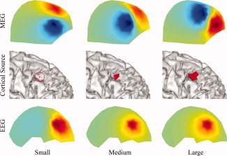
An example to illustrate the sensitivity of surface EEG and MEG in responding to spatial extent changes of cortical sources from the same location. First row: surface MEG distributions generated by simulated sources. Second row: simulated sources with varying extents from the same location. Third row: surface EEG distributions generated by simulated sources. [Color figure can be viewed in the online issue, which is available at wileyonlinelibrary.com.]

Although it is of critical significance when combining EEG and MEG to improve the performance of source reconstructions, as suggested by the simulation studies (Figs. 2, 3, 4, 5, 6, 7), the practical issue in real data analysis is how to unify EEG and MEG data to a common ground in which both types of data can be appropriately handled in solving mathematical optimization problems as stated in Eq. 7. In the present study, we used the SNR transformation [Fucks et al., 1998; Greenblatt, 1995] in the data analysis, which made EEG and MEG data unit‐free and normalized in reference to the standard deviations of noise. There are still multiple factors, such as the accuracy of noise estimations and the accuracy of volume conductors, which might impact the effective combination of EEG and MEG real data and cannot be addressed by simulation data. Furthermore, separate EEG and MEG recording sessions with the same stimulus protocol might generate differences, especially when not assessing time‐locked or phase‐locked EEG/MEG components [Yuan et al., 2010]. Considering the cost for simultaneous recordings, MEG systems are much more expensive than EEG systems, making it relatively easy to upgrade MEG facilities with additional EEG systems, but not vice versa. As a matter of fact, most MEG systems are already equipped with low‐density EEG systems (such as 20–30 electrodes). In clinical epilepsy management centers equipped with MEG systems, low density EEGs are also routinely recorded to help in the identification of interictal spikes in MEG from epilepsy patients. Despite these complexities, our results from the combined high‐density EEG and MEG data from the face recognition task demonstrate that the proposed integrative approach can successfully reveal more reliable and consistent brain activations, which are validated by our current neurophysiological knowledge and other independent measurements (i.e., fMRI). Its performance can be further improved with more sophisticated volume conductor models (e.g., FE models with anisotropy) and simultaneous EEG and MEG recordings [de Munck et al., 2007]. Thus, due to its significantly improved performance, the combined use of EEG and MEG in VB‐SCCD will be highly favored in many fields. For example, while early brain responses can be studied by simple models [Elbert et al., 1995], multiple cortical activations are expected in later latencies of brain responses, which requires more independent measurements to better characterize them. The combined EEG and MEG system will also be needed to overcome the limitations of single modality using either EEG or MEG as discussed above, such as for conditions in which accuracy and spatial resolution are of importance [Sharon et al., 2007], and when a unitary signal modality is not sensitive to brain sources [Bast et al., 2005].

It is also suggested by our simulation data that VB‐SCCD has better performance in reconstructing superficial sources than deep sources (Figs. 3, 4, 5) when both types of sources exist simultaneously in simulations. A major reason for this is that deep sources generate weaker electrical or magnetic fields compared to superficial sources when both have similar current moments. Consequently, EEG/MEG data from deep sources have lower SNRs than superficial sources since noise levels in simulations were chosen based on superposed EEG/MEG signals from multiple sources. This can lead to the degradation of localizing deep sources from multiple sources. While such simulation studies mimic realistic situations in which sources from deep brain structures might need stronger amplitudes to be identified compared to sources from epicortical structures, it does not necessarily mean that VB‐SCCD lacks the capability in reconstructing deep sources from real data. Large synchronized neural currents from deep brain parts, which can generate observable EEG/MEG signals with enough SNRs, are expected to be reconstructed as well.

To better interpret EEG and MEG source reconstruction results, statistical thresholding techniques have been proposed [Barnes and Hillebrand, 2003; Pantazis et al., 2005]. In the present study we only used a simple unified threshold to visualize all data, which might not be the best option in evaluating either simulated and or real data. Since EEG and MEG have different sensitivities to differently configured cortical sources, such a unified criterion might over‐emphasize or underestimate some sources. Although it provides a straightforward way for evaluating raw data directly from reconstructions, the integration with statistical test methods [Pantazis et al., 2005] can potentially further improve the interpretation of results.

In summary, we evaluated the performance of a novel sparse ESI technology, i.e., VB‐SCCD, using multiple modality data from EEG and MEG. Our data demonstrated that the proposed integrative approach was able to reconstruct complex brain activations supported by data from Monte Carlo simulations and experimental studies. This was achieved via the integration of independent and complimentary EEG and MEG information regarding common underlying brain sources and, mathematically, is congruent with compressive sensing theory, which happens to be the basis of our proposed sparse ESI technology. It is promising that sparse ESI technology using combined EEG and MEG can probe detailed spatiotemporal processes from complex and dynamic brain activity, and can be applied noninvasively to study large‐scale brain networks of high clinical and scientific significance.

References

- Babiloni F, Carducci F, Cincotti F, Del Gratta C, Pizzella V, Romani GL, Rossini PM, Tecchio F, Babiloni C ( 2001): Linear inverse source estimate of combined EEG and MEG data related to voluntary movements. Hum Brain Mapp 14: 197–209. [DOI] [PMC free article] [PubMed] [Google Scholar]
- Balish M, Sato S, Connaughton P, Kufta C ( 1991): Localization of implanted dipoles by magnetoencephalography. Neurology 41: 1072–1076. [DOI] [PubMed] [Google Scholar]
- Barnes GR, Hillebrand A ( 2003): Statistical flattening of MEG beamformer images. Hum Brain Mapp 18: 1–12. [DOI] [PMC free article] [PubMed] [Google Scholar]
- Bast T, Ramantani G, Boppel T, Metzke T, Ozkan O, Stippich C, Seitz A, Rupp A, Rating D, Scherg M ( 2005): Source analysis of interictal spikes in polymicrogyria: Loss of relevant cortical fissures requires simultaneous EEG to avoid MEG misinterpretation. Neuroimage 25: 1232–1241. [DOI] [PubMed] [Google Scholar]
- Baule G, McFee R ( 1965): Theory of magnetic detection of the heart's electrical activity. J Appl Phys 36: 2066–2073. [Google Scholar]
- Candes EJ, Tao T ( 2005): Decoding by linear programming. IEEE Trans Inform Theory 51: 4203–4215. [Google Scholar]
- Chapman RM, IImoniemi RJ, Barbanera S, Romani GL ( 1984): Selective localization of alpha brain activity with neuromagnetic measurements. Electroencephalogr Clin Neurophysiol 58: 2268–2275. [DOI] [PubMed] [Google Scholar]
- Cohen D, Cuffin BN ( 1987): A method for combining MEG and EEG to determine the sources. Phys Med Biol 32: 85–89. [DOI] [PubMed] [Google Scholar]
- Dale A, Sereno M ( 1993): Improved localization of cortical activity by combining EEG and MEG with MRI cortical surface reconstruction: A linear approach. J Cogn Neurosci 5: 162–176. [DOI] [PubMed] [Google Scholar]
- Darvas F, Pantazis D, Kucukaltun‐Yildirim E, Leahy RM ( 2004): Mapping human brain function with MEG and EEG: Methods and validation. NeuroImage 23: S289–S299. [DOI] [PubMed] [Google Scholar]
- de Munck JC, Goncalves SI, Huijboom L, Kuijer JPA, Pouwels PJW, Heethaar RM, Lopes da Silva FH ( 2007): The hemodynamic response of the alpha rhythm: An EEG/fMRI study. NeuroImage 35: 1142–1151. [DOI] [PubMed] [Google Scholar]
- Ding L ( 2009): Reconstructing cortical current density by exploring sparseness in the transform domain. Phys Med Biol 54: 2683–2697. [DOI] [PubMed] [Google Scholar]
- Ding L, He B ( 2006): Spatio‐temporal EEG source localization using a three‐dimensional subspace FINE approach in a realistic geometry inhomogeneous head model. IEEE Trans Biomed Eng 53: 1732–1739. [DOI] [PMC free article] [PubMed] [Google Scholar]
- Ding L, He B ( 2008): Sparse source imaging in EEG with accurate field modeling. Hum Brain Mapp 29: 1053–1067. [DOI] [PMC free article] [PubMed] [Google Scholar]
- Ding L, Zhu M, Zhang WB, Dickens DL ( 2010): Variation‐Based Sparse Cortical Current Density Imaging in Estimating Cortical Sources with MEG Data. pp 5145–5148 in Annual International Conference of IEEE–EMBS. [DOI] [PubMed]
- Ebersole JS ( 2000): Noninvasive localization of epileptogenic foci by EEG source modeling. Epilepsia 41( Suppl. 3): S24–S33. [DOI] [PubMed] [Google Scholar]
- Elbert T, Pantev C, Wienbruch C, Rochstroh B, Taub E ( 1995): Increased cortical representation of the fingers of the left hand in string players. Science 270: 305–307. [DOI] [PubMed] [Google Scholar]
- Friston K, Harrison L, Daunizeau J, Kiebel S, Phillips C, Trujillo‐Barreto N, Henson R, Flandin G, Mattout J ( 2008): Multiple sparse priors for the M/EEG inverse problem. NeuroImage 39: 1104–1120. [DOI] [PubMed] [Google Scholar]
- Fuchs M, Wagner M, Wischmann HA, Kohler T, TheiBen A, Drenckhahn R, Buchner H ( 1998): Improving source reconstructions by combining bioelectric and biomagnetic data. Electroenceph Clin Neurophysiol 107: 93–111. [DOI] [PubMed] [Google Scholar]
- Gharib S, Sutherling WW, Nakasato N, Barth DS, Baumgartner C, Alexopoulos N, Taylor S, Rogers RL ( 1995): MEG and ECoG localization accuracy test. Electroencephalogr Clin Neurophysiol 94: 109–114. [DOI] [PubMed] [Google Scholar]
- Greenblatt RE ( 1995): Combined EEG/MEG source estimation methods In: Baumgartner C, Deecke L, Stroink G, Williamson SJ, editors. Biomagnetism: Fundamental Research and Clinical Applications. Vienna, Austria: Elsevier; pp 402–405 [Google Scholar]
- Grova C, Daunizeau J, Lina JM, Benar CG, Benali H, Gotman J ( 2006): Evaluation of EEG localization methods using realistic simulations of interictal spikes. NeuroImage 29: 734–753. [DOI] [PubMed] [Google Scholar]
- Hämäläinen MS, Ilmoniemi RJ ( 1984): Interpreting measured magnetic fields of the brain: Estimates of current distributions. Helsinki University of Technology. [Google Scholar]
- Hämäläinen MS, Sarvas J ( 1989): Realistic conductivity geometry model of the human head for interpretation of neuromagnetic data. IEEE Trans Biomed Eng 36: 165–171. [DOI] [PubMed] [Google Scholar]
- Hasselmo ME, Rolls ET, Baylis GC ( 1989): The role of expression and identity in the face‐selective responses of neurons in the temporal visual cortex of the monkey. Behav Brain Res 32: 203–218. [DOI] [PubMed] [Google Scholar]
- Haxby JV, Hoffman EA, Gobbini MI ( 2000): The distributed human neural system for face perception. Trends Cogn Sci 4: 223–233. [DOI] [PubMed] [Google Scholar]
- He B ( 2004): Modeling and Imaging of Bioelectrical Activity: Principles and Applications. New York: Kluwer Academic/Plenum Publishers. [Google Scholar]
- Henderson CJ, Butler SR, Glass A ( 1975): The localization of equivalent dipoles of EEG sources by the application of electrical field theory. Electroenceph Clin Neurophysiol 39: 117–130. [DOI] [PubMed] [Google Scholar]
- Henson RN, Goshen‐Gottstein Y, Ganel T, Otten LJ, Quayle A, Rugg MD ( 2003): Electrophysiological and haemodynamic correlates of face perception, recognition and priming. Cerebral Cortex 13: 793–805. [DOI] [PubMed] [Google Scholar]
- Henson RN, Mattout J, Friston K, Hassel S, Hillebrand A, Barnes GR, Singh KD ( 2005): Distributed source localisation of the M170 using multiple constraints. in International Conference of Human Brain Mapping.
- Huang MX, Song T, Hagler DJ, Podgorny I, Jousmaki V, Cui L, Gaa K, Harrington DL, Dale AM, Lee RR, Elman J, Halgren E ( 2007): A novel integrated MEG and EEG analysis method for dipolar sources. Neuroimage 37: 731–748. [DOI] [PMC free article] [PubMed] [Google Scholar]
- Huang XH, Dale AM, Song T, Halgren E, Harrington DL, Podgorny I, Canive JM, Lewis S, Lee RR ( 2006): Vector‐based spatial‐temporal minimum L1‐norm solution for MEG. NeuroImage 31: 1025–1037. [DOI] [PubMed] [Google Scholar]
- Huiskamp G, van der Meij W, van Huffelen A, van Nieuwenhuizen O ( 2004): High resolution spatio‐temporal EEG–MEG analysis of rolandic spikes. J Clin Neurophysiol 21: 84–95. [DOI] [PubMed] [Google Scholar]
- Huizenga HM, van Zuijen TL, Heslenfeld DJ, Molenaar PC ( 2001): Simultaneous MEG and EEG source analysis. Phys Med Biol 46: 1737–1751. [DOI] [PubMed] [Google Scholar]
- Jensen O, Kaiser J, Lachaux JP ( 2007): Human gamma‐frequency oscillations associated with attention and memory. TRENDS Neurosci 30: 317–324. [DOI] [PubMed] [Google Scholar]
- Krings T, Chiappa KH, Cuffin BN, Buchbinder BR, Cosgrove GR ( 1998): Accuracy of electroencephalographic dipole localization of epileptiform activities associated with focal brain lesions. Ann Neurol 44: 76–86. [DOI] [PubMed] [Google Scholar]
- Lai Y, van Drongelen W, Ding L, Hecox KE, Towle VL, Frim DM, He B ( 2005): Estimation of in vivo human brain‐to‐skull conductivity ratio from simultaneous extra‐ and intra‐cranial electrical potential recordings. Clin Neurophysiology 116: 456–465. [DOI] [PubMed] [Google Scholar]
- Liljestrom M, Hulten A, Parkkonen L, Salmelin R ( 2009): Comparing MEG and fMRI views to naming actions and objects. Hum Brain Mapp 30: 1845–1856. [DOI] [PMC free article] [PubMed] [Google Scholar]
- Lin FH, Belliveau JW, Dale AM, Hämäläinen MS ( 2006): Distributed Current Estimates Using Cortical Orientation Constraints. Hum Brain Mapp 27: 1–13. [DOI] [PMC free article] [PubMed] [Google Scholar]
- Liu AK, Belliveau JW, Dale AM ( 1998): Spatiotemporal imaging of human brain activity using fMRI constrained MEG data: Monte Carlo simulations. Proc Natl Acad Sci USA 95: 8945–8950. [DOI] [PMC free article] [PubMed] [Google Scholar]
- Liu AK, Dale AM, Belliveau JW ( 2002): Monte Carlo simulation studies of EEG and MEG localization accuracy. Hum Brain Mapp 16: 47–62. [DOI] [PMC free article] [PubMed] [Google Scholar]
- Molins A, Stufflebeam S, Brown E, Hämäläinen MS ( 2008): Quantification of the benefit from integrating MEG and EEG in minimum L2‐norm estimation. NeuroImage 42: 1069–1077. [DOI] [PubMed] [Google Scholar]
- Morozov AV ( 1966): On the solution of functional equations by the method of regularization. Soviet Math Dokl 7: 414–417. [Google Scholar]
- Mosher JC, Leahy R, Lewis PS ( 1999): EEG and MEG: forward solutions for inverse methods. IEEE Trans Biomed Eng 46: 245–259. [DOI] [PubMed] [Google Scholar]
- Mosher JC, Lewis PS, Leahy RM ( 1992): Multiple dipole modeling and localization from spatio‐temporal MEG data. IEEE Trans Biomed Eng 39: 541–557. [DOI] [PubMed] [Google Scholar]
- Nemirovski A, Ben Tal A ( 2001): Lectures on modern convex optimization: Analysis, algorithms and engineering application: SIAM.
- Nunez PL ( 1995): Neocortical Dynamics and Human EEG Rhythms. New York: Oxford University Press. [Google Scholar]
- Okada Y, Lahteenmäki A, Xu C ( 1999): Experimental analysis of distortion of magnetoencephalography signals by the skull. Clin Neurophysiol 110: 230–238. [DOI] [PubMed] [Google Scholar]
- Pantazis D, Nichols TE, Baillet S, Leahy R ( 2005): A comparison of random field theory and permutation methods for the statistical analysis of MEG data. NeuroImage 25: 383–394. [DOI] [PubMed] [Google Scholar]
- Phillips C, Mattout J, Rugg MD, Maquet P, Friston K ( 2005): An empirical Bayesian solution to the source reconstruction problem in EEG. NeuroImage 24: 997–1011. [DOI] [PubMed] [Google Scholar]
- Scalaidhe SP, Wilson FA, Goldman‐Rakic PS ( 1999): Face‐selective neurons during passive viewing and working memory performance of rhesus monkeys: Evidence for intrinsic specialization of neuronal coding. Cereb Cortex 9: 459–475. [DOI] [PubMed] [Google Scholar]
- Sekihara K, Nagarajan SS, Poeppel D, Marantz A, Miyashita Y ( 2001): Reconstructing spatio‐temporal activities of neural sources using an MEG vector beamformer technique. IEEE Trans Biomed Eng 48: 760–771. [DOI] [PubMed] [Google Scholar]
- Sharon D, Hämäläinen MS, Tootell RBH, Halgren E, Belliveau JW ( 2007): The advantage of combining MEG and EEG: Comparison to fMRI in focally stimulated visual cortex. Neuroimage 36: 1225–1235. [DOI] [PMC free article] [PubMed] [Google Scholar]
- Shattuck DW, Leahy RM ( 2002): BrainSuite: An automated cortical surface identification tool. Med Image Anal 6: 129–142. [DOI] [PubMed] [Google Scholar]
- Sturm JS ( 2001): Using SeDuMi 1.02, a Matlab Toolbox for Optimization Over Symmetric Cones. Tilburg University, Department of Econometrics.
- Towle VL, Khorasani L, Uftring S, Pelizzari C, Erickson RK, Spire JP, Hoffmann K, Chu D, Scherg M ( 2003): Noninvasive identification of human central sulcus: A comparison of gyral morphology, functional MRI, dipole localization, and direct cortical mapping. NeuroImage 19: 684–697. [DOI] [PubMed] [Google Scholar]
- Uutela K, Hämäläinen M, Somersalo E ( 1999): Visualization of magnetoencephalographic data using minimum current estimates. NeuroImage 10: 173–180. [DOI] [PubMed] [Google Scholar]
- van Veen B, van Drongelen W, Yuchtman M, Suzuki A ( 1997): Localization of brain electric activity via linearly constrained minimum variance spatial filtering. IEEE Trans Biomed Eng 44: 867–880. [DOI] [PubMed] [Google Scholar]
- Wagner M, Wischmann HA, Fuchs M, Kohler T, Drenckhahn R ( 1998): Current density reconstruction using the L1 norm. pp 393–396 in Advances in Biomagnetism Research: Biomag96. New York: Springer‐Verlag. [Google Scholar]
- Wolters CH, Anwander A, Tricoche X, Weinstein D, Koch MA, MacLeod RS ( 2006): Influence of tissue conductivity anisotropy on EEG/MEG field and return current computation in a realistic head model: A simulation and visualization study using high‐resolution finite element modeling. NeuroImage 30: 813–826. [DOI] [PubMed] [Google Scholar]
- Yamamoto T, Williamson SJ, Kaufman L, Nicholson C, Llinas R ( 1988): Magnetic localization of neuronal activity in the human brain. Proc Natl Acad Sci USA 85: 8732–8736. [DOI] [PMC free article] [PubMed] [Google Scholar]
- Yuan H, Liu T, Szarkowski R, Rios C, Ashe J, He B ( 2010): Negative covariation between task‐related responses in alpha/beta‐band activity and BOLD in human sensorimotor cortex: An EEG and fMRI study of motor imagery and movements. NeuroImage 49: 2596–2606. [DOI] [PMC free article] [PubMed] [Google Scholar]