Detection of physiological noise in resting state fMRI using machine learning

Abstract

We present a technique for predicting cardiac and respiratory phase on a time point by time point basis, from fMRI image data. These predictions have utility in attempts to detrend effects of the physiological cycles from fMRI image data. We demonstrate the technique both in the case where it can be trained on a subject's own data, and when it cannot. The prediction scheme uses a multiclass support vector machine algorithm. Predictions are demonstrated to have a close fit to recorded physiological phase, with median Pearson correlation scores between recorded and predicted values of 0.99 for the best case scenario (cardiac cycle trained on a subject's own data) down to 0.83 for the worst case scenario (respiratory predictions trained on group data), as compared to random chance correlation score of 0.70. When predictions were used with RETROICOR—a popular physiological noise removal tool—the effects are compared to using recorded phase values. Using Fourier transforms and seed based correlation analysis, RETROICOR is shown to produce similar effects whether recorded physiological phase values are used, or they are predicted using this technique. This was seen by similar levels of noise reduction noise in the same regions of the Fourier spectra, and changes in seed based correlation scores in similar regions of the brain. This technique has a use in situations where data from direct monitoring of the cardiac and respiratory cycles are incomplete or absent, but researchers still wish to reduce this source of noise in the image data. Hum Brain Mapp , 2013. © 2011 Wiley Periodicals, Inc.

INTRODUCTION

Time‐series depicting blood oxygenation level dependent (BOLD) contrast contain complex signals arising from a variety of sources including neurovascular coupling, systemic physiology, and the magnetic resonance imaging instrument. The interpretation of functional magnetic resonance imaging (fMRI) experiments is predicated on the assumption that the measurements reflect the neurally mediated component. However, the cardiac and respiratory cycles in particular are known to contribute significant noise to the signal. The respiratory cycle causes variations from the flow of cerebro‐spinal fluid (CSF), changes in blood oxygenation and carbon dioxide levels as well as magnetic field in homogeneities because of chest motion [Birn et al., 2006; Windischberger, et al. 2002]. The cardiac cycle also causes CSF flow [Britt and Rossi, 1982] in addition to pulsation of blood vessels [Dagli et al., 1999]. It has been shown that these physiological noise fluctuations can reduce sensitivity to BOLD effects of interest [Lund et al., 2006], and with the trend towards higher‐field strengths and the concomitant increase in sensitivity of fMRI to physiological processes [Kruger et al., 2001; Triantafyllou et al., 2005] combined with emerging interest in resting state fMRI acquisition, motivation has increased for investigation of these signal sources, including their estimation and correction.

Several tools have been developed to remove fluctuations because of cardiac and respiratory cycles with the aim of increasing the (neurovascular) signal to noise, and thus reduce the number of false positive or negative voxels in the significance testing of fMRI activation paradigms. Some of these methods require modifications to the normal scanning protocol; for example, extremely fast but reduced field‐of‐view scanning to oversample the physiological cycles [Chuang and Chen, 2001], k‐space based removal methods [Wowk et al., 1997] or linking physiological cycles to the acquisition sequences [Stenger et al., 1999]. Alternatively, data driven approaches have been developed that combine BOLD sensitive imaging with simultaneous measurements of cardiac and respiratory cycles: averaging images that occur at the same stage of the cycles and removing this average from images [Deckers et al., 2006]; temporal frequency filtration [Biswal et al., 1996]; independent component analysis [Thomas et al., 2002]; and the most popular, at least by citation count, low‐order Fourier series regressions to the data [Glover et al., 2000].

Many of these removal tools rely upon physiological data acquired concurrently with the fMRI acquisition to detrend these effects. This typically takes the form of a respiratory bellows around the abdomen and a pulse oximeter placed on the fingertip or toe. Measurements of temporal variation in chest circumference and blood saturation levels are then recorded. These physiological recordings are occasionally corrupted by, e.g., subject motion, battery exhaustion, or software failure. Alternatively, physiological recording may not be available because of the unavailability of equipment or software, or if it is inappropriate to the paradigm in question (e.g., if the monitoring equipment would interfere with operation of a button box). An experimenter may only realize after data acquisition that physiological data would have been valuable, and wish to retrospectively correct the data for physiological artifacts. In each case, estimation of physiological noise is required without concomitant physiological recordings.

Some methods have been designed to function without utilizing direct monitoring of the physiological cycles. The first is the aforementioned oversampling of the frequency domain with a temporal sampling rate high enough to monitor physiological noise without aliasing, but unfortunately such short TRs do not permit acquisition of sufficient slices for whole brain coverage [Chuang and Chen, 2001]. Other methods use some form of temporal and spatial component analysis, such as PCA or ICA, [Beall and Lowe, 2007; Thomas et al., 2002] to automatically separate out differing components of the signal. Unfortunately, this requires separation of those components that are physiological in origin and those that are neurovascular, for which visual inspection is still considered by some authors to be a ‘gold standard’ [Kelly et al., 2010; Perlbarg et al., 2007]. Other methods use phase information [Cheng and Li, 2010] or the centre of k‐space [Frank et al., 2001; Le and Hu, 1996] to map physiological phase, with some success in the case of the respiratory cycle, but with more limited results when dealing with the cardiac cycle. Each of these methods shows promise but is not yet a complete solution to the problem of physiological noise removal in the absence of physiological data.

We offer an alternative means of obtaining physiological data when physiological recording is either fully or partially absent, by predicting the phase of each physiological cycle from the image data. This physiological phase data can then be used in common noise removal tools such as RETROICOR to detrend physiological noise, with comparable results to using recorded data. We demonstrate its capabilities by utilizing the predicted phase data in RETROICOR and observing its efficiency as compared to recorded physiological data.

MATERIALS AND METHODS

Removal of Physiological Noise—RETROICOR

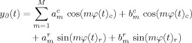
RETROICOR is a well‐cited retrospective image based correction algorithm for physiological artifact removal [Glover et al., 2000]. It works by modeling physiological noise as a low‐order Fourier function of the form:

(1)

The φ terms denote the phase of either cycle and are calculated from the output of the physiological monitoring devices. Glover et al. [2000] found empirically that M = 2 was adequate, and hence we have used the same value. The a, b are coefficients for the cardiac, c, and respiratory, r, cycles are calculated by voxelwise regression to the fMRI dataset.

In the original article by Glover et al. [2000], cardiac phase is computed as:

(2)

where t ₁ is the time of the peak of the R‐wave directly prior to time t as recorded from the cardiac recordings, and t ₂ the time for peak of the R‐wave directly after t. This assumes that the phase linearly proceeds from 0 to 2π during each R‐wave peak to R‐wave peak interval.

The respiratory phase is complicated by the significance of depth of respiration. This has been further investigated by other researchers as extensions to RETROICOR [Birn et al., 2006; Chang and Glover, 2009b; Wise et al., 2004], who found changes in respiration depth make low‐frequency contributions to fMRI data. During this investigation, we recreated the respiratory phase as measured in the original article, defined as:

(3)

where H is a histogram of the recorded respiratory values R, divided into 100 bins and rnd() is an integer rounding operation. Sgn() is the sign operator, taking values of one for arguments greater than zero, and minus one for arguments less than zero. The phase thus has a range of ±π for peak inspiration, and less for breaths of lower inspiration.

As RETROICOR removes physiological noise on a pervoxel basis, the phase of the physiological cycles for each voxel can be calculated on either a slice‐wise or volume‐wise basis. Theoretically, calculating phase on a slice‐wise basis gives a more accurate estimate of physiological noise, as the phase is more directly mapped to the time of voxel acquisition. Some studies implementing RETROICOR have therefore calculated and removed phase on a slice‐wise basis [de Munck et al., 2008; Harvey et al., 2008]. However, other studies instead have done this on a volume‐wise basis [Lund et al., 2006; Shmueli et al., 2007]. A comparative study has found that using slice‐wise timing shows small but significant improvement as compared to volume‐wise timing [Jones et al., 2008].

Throughout this work, phase was estimated on a volume wise basis, with the slice acquired TR/2 into the volume used as a timing reference. This choice was made to increase the amount of information available to the classifier at each time point. Had we chosen to conduct this work on a slice‐wise basis, the varying number of voxels per slice, and the varying level of physiological information those voxels carry, would cause predictions from different slices to have differing levels of accuracy. We also note that it may not be possible to conduct between‐subject predictions on a slice wise basis, as the match of physiological phase to an individual slice varies between acquisitions. The implications of this choice are explored in the discussion section.

In the original RETROICOR publication [Glover et al., 2000], for each voxel, the coefficients a and b were determined by a Fourier summation over all time points. The RETROICOR interpretations within publicly available research tools AFNI [Cox, 1996] and Camba [Brain Mapping Unit, University of Cambridge) implement this by estimating and detrending each physiological cycle sequentially. This technique is vulnerable to error if there are correlations between the effects of the cycles or they are aliased to similar frequencies, and so instead we estimated these simultaneously using a general linear model, as in some recent other implementations of RETROICOR [Lund et al., 2006]. Once estimated, the signal attributed to these cycles was then subtracted from the time course.

Physiological Data Restoration Using Support Vector Machines

RETROICOR relies upon accurate monitoring of the physiological cycles. However, such data may not be acquired, and in any case physiological data acquisition methods remain unreliable in modern scanner environments, and recordings are often incomplete or absent despite the imaging data being uncompromised. The effects of the physiological cycles are represented in the data, and with some knowledge of how these are represented, we can estimate the missing physiological data so that RETROICOR can be applied.

We trained a classifier on the available recorded data. We then used this model on the image data, which had no physiological recordings, to predict what those values would have been. If the predictions were sufficiently accurate, the effects of RETROICOR would be comparable to those that would have been observed had perfect recordings been possible.

In a typical physiological cycle, phase as calculated by RETRICOR proceeds from 0 to 2π before wrapping back to zero. There is therefore a mathematical discontinuity in the description of phase between 2π and 0, making it a difficult parameter to regress. Instead we chose to separate phase into discrete bins and to construct a classifier that first predicted, which phase bin each image belonged to, and then interpolated between results to obtain fine distinction.

To construct this classifier model, we assigned a phase as described earlier to each time point of the physiological recording data. Each MRI EPI‐volume was then assigned a phase based on the time point occurring in the middle of its acquisition. These volumes were partitioned into N phase bins of equal width. To determine the optimal value for N various values were tested. A multiclass support vector machine [SVM) classifier [Cortes and Vapnik, 1995; Vapnik, 1982] was then constructed that implemented a pairwise‐coupling scheme [Hastie and Tibshirani, 1998] using Platt's SVM probability estimates [Platt, 2000], as this has been previously shown to be a good multiclass SVM scheme [Duan and Keerthi, 2005]. This method allowed us to predict which phase bin, and hence which range of phase values, each EPI volume fell into.

Inputs to the classifier, both for training and testing, were whole brain volumes, preprocessed as detailed below. Each voxel was treated as a separate variable submitted to the classifiers. Aside from brain extraction, no further dimensionality reduction was performed, providing an input vector of length ∼15,000 for each time point. Class labels for each volume were then determined as described earlier, by calculating which phase bin was associated with its time of acquisition.

The analysis used an SVM algorithm based on code from SVM_light [Joachims, 1999] to generate a distinguishing model between each pair of classes (in this case each class comprised the images from a certain phase bin of a physiological cycle), using the data from the training set. SVMs are a maximum margin classifier. SVMs work by constructing a hyperplane in variable‐space that maximally splits two groups of training data. This hyperplane can then be used to predict, which group new data points belong to [Vapnik, 1982]. To account for training errors, a soft‐margin technique is used, where a user‐defined parameter ‘C’ allows for a trade off between misclassification errors and margin size [Cortes and Vapnik, 1995]. For this work, we found that increasing the value of C improved the performance of the classifier until a maximum, dataset dependent value was reached. After this value increases in C had no effect. We therefore used a value of C, 50,000, that was large enough to be greater than this maximum for all our datasets. We used a linear kernel throughout, as this produces a weight vector that can be simply displayed and averaged between subjects, to permit the between subject methodology.

The algorithm outlined by Platt converts raw SVM outputs to probabilities by modeling the SVM output as a sigmoid [Platt, 2000]. Using this method requires that the sigmoid be recalibrated and its parameters derived separately for each training dataset under consideration. We did this by using three‐fold cross validation on each training data set. Results of this cross validation were then used with a model‐trust algorithm based on that in the original description of the sigmoid fitting [Platt, 2000] to fit the sigmoid parameters for that dataset. These parameters were then recorded and used to form any predictions based on that training data set.

The pairwise coupling scheme requires a binary classifier to be created to discriminate between every possible class pair, which in this case amounts to N(N − 1)/2 binary classifiers. Once each classifier has returned a value and its output converted to a Platt probability (r _{i j}, where i and j are the two classes the classifier discriminates between), pairwise coupling attempts to estimate the underlying class probabilities from these binary outputs. We do this by introducing variables μ_{i j} where:

(4)

and p _i is the probability (to be found) that the test image lies in group ‘i’. Initial estimates of p _i were set as uniform [e.g., 1/(number of classes)]. The p _i values are then optimized such that these μ_{i j} values are as close to the r _{i j} as possible. In practice, using the Kullback–Leibler distance as a measure of proximity between r _{i j} and μ_{i j}, the probabilities are found from:

(5)

This is repeated until convergence, defined by an average difference in p _i between successive iterations of less than 0.001, renormalizing p _i after each iteration. In this equation n _ij is the number of training instances that were either in group ‘i’ or group ‘j’.

This technique provided an optimized class probability, p _i, for membership of each possible class. Selecting the class with highest probability would therefore result in a prediction with resolution equal to the class width (2π/N). We improved this resolution by fitting a cubic spline to the class probabilities, and the prediction was derived from the phase value corresponding to the peak of the fitted spline. Each 3D volume submitted to the classifier therefore produced a single scalar prediction, which could take any value in the continuous range 0–2π, regardless of the chosen value of N. We chose to use a interpolation resolution of 0.1 radians throughout the results presented in this work, as little benefit was seen from choosing finer resolution.

No temporal smoothing of results was attempted, as aliasing of the physiological cycle meant that each time point carried little information that could be used to improve the prediction of its neighbors.

Experiments

To assess the physiological phase prediction technique, we tested it on resting state data with concurrently acquired physiological recordings. We repeated this for both split half cross validation within the same dataset (‘partially absent data/within‐subject training’) and leave one out cross validation over all data sets (‘fully absent data/between‐subject training’). Accuracy of the algorithm was tested by measuring root mean squared error and Pearson product‐moment correlation between predicted and recorded values. Testing of its efficacy at removing physiological noise was undertaken by using RETROICOR on the datasets with either predicted or recorded values. Resulting datasets were compared using a Fourier transform of the data, and seed based correlation analysis (SCA).

Finally, a weight vector based on the predictive models was computed, demonstrating the regions of the brain weighted most strongly in predictions of the physiological cycles.

Study Participants and MRI Data Acquisition

Scans were acquired from 27 healthy volunteers with ages 22–43 years (mean 30 ± 6), of whom 3 were female. The measurements were performed on a 3 T Siemens MAGNETOM Trio scanner (Siemens, Erlangen, Germany) with an 8‐channel phased‐array head coil. For acquisition of the resting state fMRI data, the subjects were told to lie still in the scanner with their eyes closed. Functional time series of 488 time points were acquired with an echo‐planar imaging sequence. The following acquisition parameters were used: echo time = 25 ms, field‐of‐view = 22 cm, acquisition matrix = 44 × 44, isometric voxel size = 5 × 5 × 5 mm³. Twenty‐six contiguous interleaved axial slices covered the entire brain with a repetition time of 1,250 ms (flip angle = 70°). High resolution T1‐weighted structural MRI scans of the brain were acquired for structural reference using a 3D‐MPRAGE sequence (TE = 4.77 ms, TR = 2,500 ms, T1 = 1,100 ms, flip angle = 7°, bandwidth = 40 Hz/pixel, acquisition matrix = 256 × 256 × 192, isometric voxel size = 1.0 mm³).

An additional dataset was taken with a single subject (male, aged 26 years) on a 3 T Siemens MAGNETOM Trio scanner (Siemens, Erlangen, Germany) on a different site. This dataset was taken to allow comparison between results with the above acquisition parameters, and those that may be found with alternate acquisition parameters. Two resting state sessions with closed eyes were acquired, both 10 min and 10 s in length using a 12‐channel phased‐array head coil. An echo‐planar imaging sequence was used with parameters as close as possible to the original acquisition for one run, except using a 64 × 44 matrix, maintaining the same (5 × 5 × 5 mm³) spatial resolution with a larger field of view. All other parameters were identical. For the second run, instead the following were used: echo time = 30 ms, field of view = 19.2 cm, acquisition matrix = 64 × 64, voxel size = 3 × 3 × 3 mm³. Thirty‐two interleaved axial slices of size 3 mm and slice gap 0.75 mm covered the entire brain with a repetition time of 2,000 ms (flip angle = 70°). All analysis on this dataset was identical to that which took place on the larger dataset. Results from this dataset are presented in Supporting Information.

The study was undertaken in compliance with the Code of Ethics of the World Medical Association (Declaration of Helsinki) and was approved by the local IRB of the medical school, Otto von Guericke University, (or the Wolfson Brain Imaging Centre, University of Cambridge for the single subject data) with all participants giving written consent prior to scanning.

Data Preprocessing

The first 10 s of each imaging sequence were discarded to allow for T1‐magnetization stabilization. Motion correction (rigid body translation and rotation) and brain extraction was then performed using Camba (Brain Mapping Unit, University of Cambridge).

Estimation of Phase of Physiological Cycles

The monitoring hardware was the manufacturer's standard equipment—a respiratory bellows and pulse oximeter—and measured chest expansion and blood oxygen saturation as proxies for the respiratory and cardiac cycles, respectively. This data was taken concurrently with fMRI acquisition. The physiological monitoring device sampled each cycle at a frequency of 49.82 Hz (50.0 Hz for the single subject dataset) and a time stamp on the output allowed temporal registration to the BOLD time series.

A phase value for each time point of the physiological monitoring data was calculated using the AFNI toolbox [Cox, 1996] based on this data.

Prediction of Physiological Phase

Recreation of partially absent data/within‐subject training

In some situations—for example if a subject were to move the body part with physiological monitoring device attached or device batteries were exhausted—only partially useable data is recorded from physiological monitoring apparatus. In this case, RETROICOR could only be applied to the data before the loss of physiological recording. Using the methods described earlier, we created a SVM model from a subset of our full dataset and recreated the physiological data for the remaining images, so that RETROICOR could instead be applied to the whole dataset.

Classifiers were trained on the first 240 time points and tested on the latter 240 time points of each subject's dataset. For each prediction, multiples of 2π were added/subtracted until the result lay within ±π of the recorded value. This does not affect the RETROICOR implementation, as it uses sinusoids of the phase, but enables meaningful comparisons between predicted and recorded phase.

When implemented with RETROICOR, we did not include the half of the data that had been used to train the SVM model in our RETROICOR analysis. This meant that effects were only from the predicted values, and were not obscured by contributions from recorded values on the first half of the data.

Prediction of values using split within‐subject training was repeated, reducing the amount of training data each time, to determine what level of training data would be required to obtain good results. This was done by removing time points from the start of the dataset each time. The values sampled were 240 (all of the data), 200, 160, 120, 80, 40, 30, 20, or 10 time points used as training.

Recreation of fully absent data/between‐subject training

A leave‐one‐out procedure was adopted in which the entire 480 time‐points from all subjects, except one, were used for training a set of classifiers. Weight vectors of classifiers were then averaged across subjects at each point in MNI space [Evans et al., 1993]. These average classifiers were then registered into the remaining subject's brain space using FLIRT [Jenkinson and Smith, 2001], and used to predict the physiological data for that subject's entire time course.

Aside from the source of the training data, all other techniques used were the same as for the case of partially absent data.

This was repeated for each subject, retraining on the remaining 26 subjects each time.

Benchmark for predictions using random number generation

To provide a baseline with which to compare performance of the predictions, we also used a pseudo‐random number generator to homogeneously distribute predictions between ±π of the recorded values. This was repeated 100 times for each data set, for each physiological cycle.

Comparing Recorded to Predicted Physiological Phase

To determine how accurate the physiological phase predictions were, we first of all directly compared them to the recorded values. For each subject, we calculated the root mean squared error (RMSE) between predicted and recorded values.

Example plots of predicted phase plotted against recorded phase, from the single subject with the median RMSE score, are presented.

As with all the following methods, this was repeated for both cycles (cardiac and respiratory) and both types of prediction (partially and fully absent physiological data). In only this method we also compared over all sampled numbers of phase bins, and to the pseudo‐random number generator.

Fourier Transform

As a simple first comparison of RETROICOR performance with recorded and predicted phase values, we computed the Fourier transform of each voxel's time course before and after RETROICOR with each type of physiological data, and then averaged these across the whole volume. Comparison of these Fourier transforms then shows how much each RETROICOR implementation has reduced signal fluctuations at different frequencies. The aim was to demonstrate whether predicted physiological phase allowed RETROICOR to remove the same spectral components as using recorded physiological phase.

Example plots of a single subject with median RMSE error are presented for comparison.

Seed Based Correlation

We then chose an analysis technique that has been used to study resting state data to show how either RETROICOR technique could affect a standard data analysis. The analysis we chose was seed based correlation [Cordes et al., 2000; Uddin et al., 2009], using a seed region for the default mode network, as taken from [Fox et al., 2005]. Seed based correlation works by calculating the correlation coefficient between individual voxel time courses and the time course of the seed region. The intent of the method is to therefore infer some kind of relationship between the voxels of brain matter encompassed by the seed region and other voxels displaying high correlation to the seed voxel. Here we show how correlation between voxels and a seed in the default mode network may vary with RETROICOR based on different physiological data.

To conduct seed based correlation, we followed a simplified SCA methodology. Following the above preprocessing steps, we either (a) performed no physiological noise removal, (b) performed physiological noise removal with recorded phase values or (c) performed physiological noise removal with predicted phase values. We then transformed each subject time course into standard MNI space. We calculated an average time course of a cubic seed region of sides 7 mm centered on a seed voxel from the posterior cingulated cortex (PCC). We used the same voxel used in at least two prior studies [Cole et al., 2010; Fox et al., 2005], where it was given, respectively, Talairach coordinates of (−2, −36, 37) and MNI coordinates of (−2, −39, 38). On a voxelwise basis, the correlation coefficient was then calculated between the seed time course and all voxel time courses. This was repeated for all subjects. Finally, correlation coefficients were averaged over all subjects for each voxel.

This is a simplified SCA method, in that we did not conduct temporal filtration, global signal regression, CSF regression or any of the other preprocessing steps that are sometimes applied to analyses of this sort. It has been suggested that if used, these steps should be applied after physiological corrections [Strother, 2006]. As we were solely interested in the differences elicited by using the different physiological correction schemes, we did not conduct these further preprocessing steps, which might blur the differences of interest.

Weight Vectors

When using linear SVMs, the weight vector demonstrates regions that the model uses most in its predictions. Regions of large magnitude in the weight vector have the most impact on eventual predictions. In the scheme used here, there are multiple weight vectors as each phase bin is compared to each other. We can gain an insight into how the physiological effects on the fMRI image change over time, however, by looking at weight vectors from classifiers that distinguish between adjacent phase bins. For example, in a 10 phase bin system, a weight vector of the classifier comparing phase bin one to phase bin two shows the voxels most useful in distinguishing between images of the brain seen during the first and second tenths of the physiological cycle. This can then be repeated over all adjacent phase bins to give a time series of weight vectors. We calculated the weight vectors for the N = 10 case (the highest value of N sampled) to give the finest temporal resolution available. The time series of weight vectors for the cardiac and respiratory cycles, averaged over all subjects, are then presented individually.

RESULTS

Unless otherwise stated, all results presented here are average ± one standard deviation.

Comparing Recorded to Predicted Physiological Phase

For both cycles, RMSE was reduced by using N greater than two (Fig. 1). N > 3 did not give significantly differing results, either in terms of average error or correlation coefficient, compared using a paired two tail t‐test with P < 0.05 as a threshold.

Figure 1.

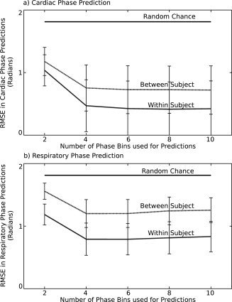
Graphs of root mean squared error (RMSE) in predictions of (a) cardiac and (b) respiratory phase. In each graph, black line displays results from the benchmark predictions using random number generation, the dashed gray line displays results from between‐subject training (median values), and the solid gray line (lowest values) displays results from within‐subject training. In each case, error bars are ± one standard deviation (error bars on random number generation results too small to plot).

In every case, the random number benchmark gave RMSE larger than the predictions. The cardiac cycle when predicted using within subject training provided the lowest RMSE, with highest RMSE when predicting the respiratory cycle using between subject training. This last case was the only one for which (if N > 3) the RMSE was greater than half that of the random number generation benchmark, and has a visibly worse match to recorded phase in example scatter plots (Fig. 2d). The other cases, prediction of cardiac cycle with between subject training and prediction of respiratory cycle using within subject training lay in between these two extreme cases.

Figure 2.

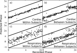
Example plots of predicted phase against recorded phase for the cases of (a) the cardiac cycle, with a classifier trained within a subject's data, (b) cardiac cycle, classifier trained between subjects, (c) respiratory cycle, classifier trained within a subject, and (d) respiratory cycle, classifier trained between subjects. The data is from the single subject with median RMSE in predictions made from classifiers trained between‐subjects. All cases used six phase bins to make predictions (N = 6). Solid dark lines represent ±π of the recorded values. This is the limit of possible error on each prediction, as factors of 2π were added or subtracted until each prediction lay within this range.

As examples, in Figure 2 are scatter plots of predicted against recorded phase for single subjects. These are median subjects in each case; the predictions have median RMSE error amongst our subjects, meaning as many fits were worse than this as were better than this. In each plot the N = 6 case is presented as a representative sample, as it is roughly central amongst the N = 4, 6, 8, and 10 cases. These cases showed less than 5% difference in RMSE and as such did not demonstrate notably different behavior in example plots. Pearson correlation coefficient scores for the relationship between recorded and predicted phases were, in these cases, 0.99 (mean: 0.96 ± 0.08 over all subjects) for the cardiac cycle predicted after training within the subject, 0.93 (mean: 0.93 ± 0.08 over all subjects) for the cardiac cycle predicted after training between subjects, 0.96 (mean: 0.92 ± 0.04 over all subjects) for the respiratory cycle predicted training within the subject and 0.83 (mean: 0.85 ± 0.05 over all subjects) for the respiratory cycle predicted after training between subjects. By contrast, the benchmark random number generator produced an average correlation score of 0.70. This nonzero correlation score from the random number generator was the result of shifting each prediction such that it lay between ±π of the true value. Supporting the evidence of Figure 1, again the relationship between recorded and predicted phase was strongest for cardiac predictions using within subject training, and worst for respiratory predictions with between subject training.

When the level of training data was reduced from 240 TRs (300 s), the RMSE of predictions increased (Fig. 3). This data is again from the N = 6 case, as the behavior of the cases was very similar regardless of the chosen value of N. The RMSE was significantly increased (P < 0.05, paired t‐test, d.o.f. 26) for the cardiac cycle when using any amount of training data less than the maximum, or if using less than 200 s of training data for the respiratory cycle.

Figure 3.

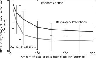
Graph of root mean squared error (RMSE) in predictions of cardiac (light gray) and respiratory (dark gray) phase from fMRI data as amount of training data is reduced. Also displayed is a line (black) indicating the RMSE error resulting from random chance predictions of physiological phase. Means and errors (±one standard deviation) are taken over all subjects. In each case, data was removed from the start of the training set until the desired amount was left. A model was then trained on this data, and used to predict physiological phase for the entirety of the second half of the dataset. The model used in this case takes a value of N = 6.

Fourier Transform

The Fourier transforms were averaged over all voxels that had been extracted by the brain extraction tool (Fig. 4). Datasets presented use N = 6 and are of the single subject with median RMSE between the two physiological cycles for the fully absent data/between subject training. This means as many predictions had greater error than these examples as had lesser error. These examples are representative of the behavior in the overall group, though the frequency at which the physiological cycles aliased into the spectra varied between subjects.

Figure 4.

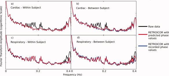
Example Fourier Transforms of dataset with median RMSE in predictions. In each plot, the black line displays the raw (no RETROICOR) data, blue line displays data after RETROICOR has been applied using recorded physiological phase values and red line displays data after RETROICOR has been applied using predicted physiological phase values. The plots show (a) detrending of the cardiac cycle using predicted values created by training within the subject's data, (b) detrending of cardiac cycle using predicted values from training between subjects, (c) detrending of respiratory cycle using predicted values created by training within the subject's data, and (d) detrending of respiratory cycle using predicted values from training between subjects. Each was calculated based on the last 240 time points in each dataset. Fourier transforms of the physiological monitoring data showed that the cardiac cycle has a fundamental frequency that varied in the approximate range 0.95–1.5 Hz (aliased to 0.15–2.5 Hz in the fMRI data), whilst the respiratory cycle had a fundamental frequency between 0.35 and 0.42 Hz. [Color figure can be viewed in the online issue, which is available at wileyonline library.com.].

As can be seen from the example Fourier transforms, when using RETROICOR with either predicted or recorded physiological values, the Fourier transform showed reduced power from spikes in two main regions of the spectrum. When cardiac cycle detrending was applied with RETROICOR, spikes around 0.2 Hz were reduced in amplitude (Fig. 2a,b), when using either predicted or recorded cardiac phase values. Similarly, when respiratory cycle detrending was applied with RETROICOR, spikes around 0.4 Hz were reduced in amplitude (Fig. 2c,d), when using either predicted or recorded cardiac phase values.

The biggest discrepancy between using recorded and predicted physiological values came when removing respiratory noise with between‐subject testing. Figure 4 shows that in this case there is a discrepancy between the Fourier transforms around the 0.35–0.4 Hz region. This is reinforced by the percentage signal changes computed in Table I. This table shows that the percentage of signal change caused by using RETROICOR, in the relevant regions, is very similar using either source of physiological phase. The discrepancy between the effects of the two RETROICOR implementations is smaller than this, except in the case of predicting the respiratory cycle between subjects. This follows the evidence of the previous results, where the fit for predictions was good except in the case of the respiratory cycle trained between subjects.

Table I.

Percentage signal changes between spectra without RETROICOR denoising, (raw) with RETROICOR denoising using recorded physiological monitoring values (RETROICOR with recorded values) and with RETROICOR denoising using predicted physiological monitoring values (RETROICOR with predicted values)

	Within‐subject training		Between‐subject training
	Cardiac	Respiratory	Cardiac	Respiratory
Raw data versus RETROICOR with recorded values	12 ± 11%	18 ± 15%	11 ± 10%	17 ± 14%
Raw data versus RETROICOR with predicted values	12 ± 11%	17 ± 15%	9 ± 9%	10 ± 8%
RETROICOR with predicted values versus RETROICOR with recorded values	1 ± 1%	4 ± 3%	4 ± 3%	11 ± 10%

In each case, percentage signal change is calculated from the dataset in Figure 4, and is averaged over all frequencies in the range approximately associated with the respective physiological cycles for that dataset. These are 0.15–0.25 Hz for the cardiac cycle and 0.35–0.4 Hz for the respiratory cycle.

Seed Based Correlation

After using RETROICOR with either recorded or predicted values, correlation coefficients in SCA changed throughout the brain (Fig. 5). Figure 5a,d show the raw Pearson correlation scores with the seed region, resembling the often reported ‘default mode network’ [Cole et al., 2010; Uddin et al., 2009].

Figure 5.

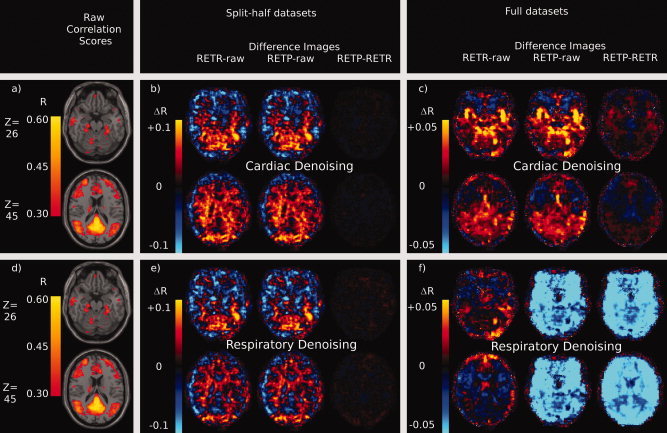
Effects of RETROICOR using recorded or predicted physiological phase values on voxelwise Pearson correlation scores with a seed timecourse in the PCC. Raw correlation scores are thresholded at 0.3 (uncorrected) and displayed (a, d) overlaid on an MNI structural atlas. Figures a and d are identical and are repeated for reference. RETROICOR was then used to remove the effects of the cardiac cycle (b, c) or the respiratory cycle (e, f) and correlation scores were recalculated. Difference images were calculated by comparing the average correlation score in each voxel from two of the following three preprocessing steps: RETROICOR with recorded phase values (RETR), RETROICOR with predicted phase values (RETP) or no physiological noise removal (raw). For each figure the leftmost image is of the RETR‐raw difference image, then the RETP‐raw image, with RETP‐RETR rightmost. The case where only half the data set was used (within subject training for prediction) is demonstrated for cardiac cycle (b) and respiratory cycle (e) noise removal. The case where all data was used (between subject training for prediction) is displayed for the cardiac cycle (c) and respiratory cycle (f) also. [Color figure can be viewed in the online issue, which is available at wileyonlinelibrary.com.].

Difference images show that RETROICOR causes similar changes in these R scores, whether using recorded or predicted values, if predictions are made by training within a subject's own data (Fig. 5b,e). The magnitude of R difference caused by using predicted phase values as opposed to recorded phase values was typically only a tenth of the magnitude of the difference seen when using RETROICOR in the first place.

When using predictions made after training between subjects, the differences caused by using predicted as opposed to recorded values with RETROICOR grew larger. With cardiac detrending, the differences between using recorded and predicted values grew to nearly half of the magnitude of the differences seen using RETROICOR in the first place (Fig. 5c).

The largest differences between using predicted and recorded values were seen, as in the previous results, in predicting the respiratory cycle using between subject training (Fig. 5f). In this case the differences in R scores caused by using predicted as opposed to recorded phase values were larger than the differences caused by using RETORICOR. This is further evidence for poorer predictions in the case of predicting the respiratory cycle between subjects.

Weight Vectors

The weight vector for both the cardiac and respiratory cycles (Fig. 6a,b) show greatest amplitude in regions typically associated with physiological noise in fMRI‐ventricles, cerebrovasculature, and the brain edge. There is no region of the brain with consistently low‐weight; however, indicating that all voxels are used to some degree in making predictions. In particular the cardiac cycle weight vector (Fig. 6a) demonstrates a band of high weight moving in the superior–inferior direction across time points, involving large numbers of voxels in predictions.

Figure 6.

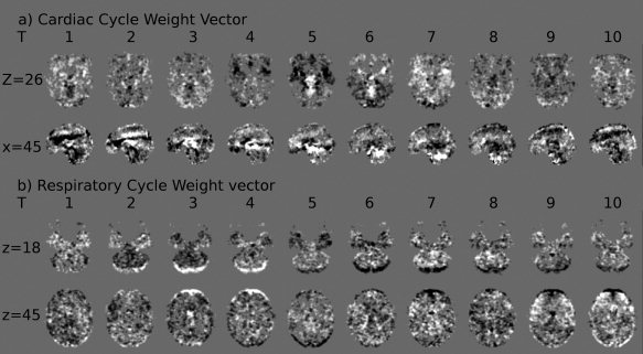
Average weight vectors from the classifiers using 10 phase bins to predict (a) cardiac phase and (b) respiratory phase. Time points (T) 1–10 represent weight vectors distinguishing between adjacent phase bins, e.g., T = 5 depicts the weight vector distinguishing between images acquired during phases 4π/5−π and images acquired during phases π−6π/5. Weight vectors from classifiers distinguishing between nonadjacent phase bins have been omitted. Mid gray (background color) represents a weight vector value of zero—no impact on predictions, bright values represent voxels where brightness indicates weighting towards the later phase bin, dark values represent voxels where brightness indicates weighting towards the earlier phase bin discriminated by the particular classifier. As weight vectors at each time point, and for each physiological cycle, were separately derived, direct comparison of intensity values between them is not possible. Each image uses the same arbitrary scaling.

DISCUSSION

We have demonstrated that predictions can be made from data in the image domain, to track physiological phase on a time point by time point basis, and thus detrend physiological noise, without need for the standard monitoring equipment. From the results it can be seen that there exists a relationship between physiological phase as calculated by RETROICOR, and fMRI image data. If this were not the case, the average prediction would have been no better than chance. This is supported by previous work showing noise linked to the physiological cycles in fMRI data [Birn et al., 2006; Dagli et al., 1999; Windischberger et al., 2002].

We found in general that predictions made using a classifier ensemble trained on a subject's own data (partially absent data case) performed better than a classifier ensemble averaged over multiple other subjects (fully absent data) (Figs. 1 and 2). The response of a brain to the physiological cycles contains many subject‐specific influences, such as depth of respiration, heart rate, ventricle size and cerebrovascular network architecture that influence fMRI response, causing this increased difficulty in making predictions ‘between’ subjects. We have not tested whether between‐session changes in response to physiological cycles are smaller than between‐subject changes. We would, however, expect this to be the case as between‐subject scans are of necessity also between‐session, incorporating both the variability associated with multiple sessions and the subject specific influences mentioned above. This implies that, where possible, for optimal physiological detrending using these techniques, at least some physiological data from a subject should be taken. The results from using reduced levels of training data show that the more of this data that can be acquired, the better the results will be. Errors rapidly increased if less than 100 s of training data was used, and so we regard this as a minimum, with a preference for more data if possible. Even if this is not possible during the acquisition of the time series to be detrended, recording during another time series would likely give a better estimation of the effects of physiological cycles on that subject than relying on similarities between their response and the general population average. This may be the case, for example, if the fMRI task requires the use of button pressing or hand motion, making the use of a pulse‐oximeter or respiratory bellows problematic for a specific paradigm, but not in general.

Despite this reduction in prediction accuracy, the Fourier transforms for the case of fully absent data show good similarity between RETROICOR implemented on predicted and recorded values, at least in the case of the cardiac cycle (Fig. 4). Notably, noise in the frequency region associated with the respiratory cycle is reduced less when using predicted values. This is supported by evidence from SCA (Fig. 5), that showed similar changes in correlation coefficient after RETROICOR with either recorded or predicted values of the cardiac cycle, but not the respiratory cycle. Taken with the poorer relationship between predicted and recorded data in this case, the results indicate that the respiratory cycle is more variable between subjects than the cardiac cycle. Although, using predictions in this case does still reduce some level of the respiratory noise seen with a Fourier transform, a complementary technique, such as the phase or k‐space estimation methods [Cheng and Li, 2010; Frank et al., 2001; Le and Hu, 1996], may be a better choice for respiratory noise reduction in the case of fully absent physiological data. In the case of partially absent data, this machine learning based technique is appropriate for use with the respiratory cycle.

The reasons for greater respiratory between‐subject variation stem from multiple factors. The first is that the effects on fMRI are partially resulting from field changes as the subject's chest moves. Subject chests show considerable variability, leading to variable effects on fMRI images. Secondly, subjects have variable breath depths, meaning that effects on fMRI images will have considerably different magnitudes between subjects. The topic of respiratory depth variation and fMRI is a current field of study, [Birn et al., 2009; Chang and Glover, 2009b] and it is apparent that respiration depth changes do cause variation in fMRI images, even over a single time course. The variation between subjects can be expected to be even larger, leading to greater error in predictions that implicitly assume similar responses between subjects. Thirdly, the particular physiological monitoring system that was used auto‐corrects to prevent the respiratory signal from saturating. This will render the calculation of respiratory phase, as presented in the original RETROICOR paper, problematic, as it attempts to account for respiration depth, but the auto‐correction makes this impossible to discern. The cardiac cycle suffers such problems to a lesser extent, and is why the prediction scheme had better performance on between subject predictions.

For the case of partially absent data most of these concerns are not relevant, and the Fourier transforms and seed based correlation analyses show that the predictions in this case give comparable performance to using recorded values, and so would be a good technique to use.

The weight vectors (Fig. 6), corroborated by the maps of where SCA showed changes after RETROICOR (Fig. 5) show broad agreement with previous reports that the cardiac cycle induces noise mainly in CSF and cerebrovasculature, and the respiratory cycle primarily affects the brain edge and CSF [Dagli et al., 1999; Windischberger et al., 2002]. These are some of the regions with highest amplitude in the relevant weight vectors, demonstrating that these are regions that the model is using to distinguish between different parts of the two cycles. High‐values of the weight vector, and regions of large change in correlation coefficient after RETROICOR, were not strictly localized to these regions, however. Instead, all regions of the brain had at least some changes in correlation coefficient (Fig. 5) and contribution to the predictions (Fig. 6), underlining the importance of using physiological detrending, even in regions not typically associated with high physiological noise. It should be noted that although we can state that a whole weight vector shows ability to discriminate physiological phase, the same cannot be said of individual voxel values within that weight vector. The SCA analysis also used an abbreviated preprocessing pipeline. These factors limit the scope of comparisons that can be made to prior investigations, utilizing different methodology, in both cases.

The weight vector showed a band of high amplitude moving in the superior–inferior direction over time in the cardiac cycle. We are not able to fully explain this phenomenon; however, we suggest this could demonstrate a bolus of blood passing through the brain, causing intensity changes over time. This would not necessarily be visible in prior studies of cardiac effects because of its seemingly short duration (single voxels experience positive and negative lobes of the band in subsequent time points). In the weight vector for the respiratory cycle, a rotation component is apparently present, indicating a ‘nodding’ action of the subjects throughout the respiratory cycle. This demonstrates that motion correction software may not be capable of removing all gross motion of the head associated with the respiratory cycle.

It is difficult to compare these results to those seen in prior studies of the use of physiological noise removal with resting state data [Birn et al., 2006; Chang and Glover, 2009a; Van Dijk et al., 2010] as typically prior studies only report changes in terms of significance, whereas we were interested in magnitude of changes regardless of significance measures. We did, however, generally see increases in correlation in regions often associated with the default mode network (Fig. 5) when using RETROICOR, which agrees with findings of previous reports.

We were interested to note that using RETROICOR on the full and half data sets had slightly different effects in general on seed based correlation values (Fig. 5b,c,e,f). The causes of this are beyond the scope of this investigation, and it is not clear whether this will hold true of SCA investigations in general, or is an artifact of our datasets in particular. We do note, however, that the basic RETROICOR methodology we used is expected to be less stable over long periods, as changes in respiratory or cardiac rate are not adequately modeled, but have been demonstrated to affect fMRI datasets [Birn et al., 2006; Shmueli et al., 2007]. We also note that, the full datasets would allow greater information for the determination of the Fourier components in the RETROICOR methodology. These effects, and their interactions, could explain some of the differences.

The technique as demonstrated shows promise for use in situations where physiological data could not be recorded, or recording was corrupted. It has demonstrated a close fit to values obtained by actually recording the cycles, giving it practical use for experimenters. However, it is bounded by the same limitations as the RETROICOR technique. Amongst these are the previously mentioned variations in cardiac and respiratory rate, which RETROICOR does not take into account. Interaction terms between the cardiac and respiratory cycle are not used in the original RETROICOR formulation, and hence have not been included in this study, but interactions have been shown to be present [Frank et al., 2001], and attempts have been made to model and remove these effects as extensions to RETROICOR [Brooks et al., 2008; Harvey et al., 2008]. It has been shown that end tidal CO₂ monitoring offers insights into the effects of the respiratory cycle on fMRI that a respiratory bellows does not entirely account for [Chang and Glover, 2009b]. It is unknown how well a predictive technique, such as the one outlined herein, could model these values. The incorporation of these factors into the machine learning model will be important next steps towards detrending of the physiological cycles in the face of problems monitoring them.

The data analysis discussed so far has taken place on data with specific acquisition parameters and from only one scanner. We acquired additional data from a single subject, using two different sets of acquisition parameters, one matched to those used in the main body of this work (referred to as TR = 1.25 s parameters) and one with different acquisition parameters (referred to as TR = 2 s parameters, see ‘Materials and Methods’ section for further details of exact parameters used). This dataset allowed us to minimize between‐subject variability in our comparison between acquisition parameters. The results of this analysis are presented in the Supporting Information. The RMSE of predictions took very similar values with either set of acquisition parameters (Figs. S1 and S2), with the difference between the two far less than the standard deviation over the multi‐subject dataset presented above (Fig. 1). The effects on the Fourier transforms were likewise similar between the two datasets (Fig. S3, Table S1). The SCA maps (Fig. S4) provide more evidence that the predictive scheme operates in a similar manner on the dataset with different acquisition parameters: the difference between RETROICOR implementations was smaller than the difference produced by using any RETROICOR implementation by itself.

More data is required to fully establish whether the methods presented in this work are equally valuable at differing acquisition parameters than those presented. However, the close match between results seen in these two datasets with differing parameters does provide promising initial evidence, leading us to expect this technique to work comparably well in larger datasets with acquisition parameters such as those in the TR = 2 s dataset.

We chose to predict phase on a volume wise, rather than slice wise basis. Using slices instead to make predictions would reduce the reliability of each prediction, by reducing the number of voxels available to the classifier at each time point to the number in an individual slice. We note that slice‐wise prediction would potentially allow for some temporal smoothing by oversampling each physiological cycle. However, the means by which these less reliable, and variable predictions (as each slice contains varying levels of information on the physiological cycles) could be integrated into a cohesive output are not clear to us at present. A pilot study we undertook, attempting to utilize slice‐wise predictions, produced results with greater errors than those demonstrated in this work. Using volume‐wise timing is a known approximation to the technique; however, a comparative study, focused on optimizing RETROICOR implementation, found that in real data the difference between slice‐wise and volume‐wise phase calculation for RETROICOR, though significant, was minimal, [Jones et al., 2008]. We therefore believe that this approximation had little effect on results.

The technique at present is a useful tool for removing periodic variation caused by the physiological cycles, if some subject specific physiological and fMRI data is available. If no physiological data is available with fMRI data, the technique can still predict the cardiac cycle well, but not the respiratory cycle.

CONCLUSIONS

We have presented a technique for the prediction of phase of the cardiac or respiratory cycles from fMRI image data. This has use in the detrending of physiological noise from the fMRI data in the absence of directly recorded information on the physiological cycles.

The technique showed a good match to recorded values if it was trained on the same subject it was tested on. For the respiratory cycle performance deteriorated if it was instead trained on other subjects, but for the cardiac cycle still demonstrated a good fit to recorded data.

Using RETROICOR with the predicted values showed similar performance to using it with recorded values, excepting the case of the respiratory cycle predicted after training on subjects other than the one being tested on. This was tested by taking Fourier transforms of data and performing SCA before and after RETROICOR using either predicted or recorded physiological phase values.

The technique has potential use as a means of performing physiological detrending on data sets where full physiological monitoring was not possible.

Supporting information

Additional Supporting Information may be found in the online version of this article.

Supporting Information Figure 1.

Supporting Information Figure 2.

Supporting Information Figure 3.

Supporting Information Figure 4.

REFERENCES

- Beall EB, Lowe MJ ( 2007): Isolating physiologic noise sources with independently determined spatial measures. Neuroimage 37: 1286–1300. [DOI] [PubMed] [Google Scholar]
- Birn RM, Diamond JB, Smith MA, Bandettini PA ( 2006): Separating respiratory‐variation‐related fluctuations from neuronal‐activity‐related fluctuations in fMRI. Neuroimage 31: 1536–1548. [DOI] [PubMed] [Google Scholar]
- Birn RM, Murphy K, Handwerker DA, Bandettini PA ( 2009): fMRI in the presence of task‐correlated breathing variations. Neuroimage 47: 1092–1104. [DOI] [PMC free article] [PubMed] [Google Scholar]
- Biswal B, DeYoe AE, Hyde JS ( 1996): Reduction of physiological fluctuations in fMRI using digital filters. Magn Reson Med 35: 107–113. [DOI] [PubMed] [Google Scholar]
- Britt RH, Rossi GT ( 1982): Quantitative analysis of methods for reducing physiological brain pulsations. J Neurosci Methods 6: 219–229. [DOI] [PubMed] [Google Scholar]
- Brooks JCW, Beckmann CF, Miller KL, Wise RG, Porro CA, Tracey I, Jenkinson M ( 2008): Physiological noise modelling for spinal functional magnetic resonance imaging studies. Neuroimage 39: 680–692. [DOI] [PubMed] [Google Scholar]
- Chang C, Glover GH ( 2009a): Effects of model‐based physiological noise correction on default mode network anti‐correlations and correlations. Neuroimage 47: 1448–1459. [DOI] [PMC free article] [PubMed] [Google Scholar]
- Chang C, Glover GH ( 2009b): Relationship between respiration, end‐tidal CO2, and BOLD signals in resting‐state fMRI. Neuroimage 47: 1381–1393. [DOI] [PMC free article] [PubMed] [Google Scholar]
- Cheng H, Li Y ( 2010): Respiratory noise correction using phase information. J Magn Reson Imaging 28: 574–582. [DOI] [PubMed] [Google Scholar]
- Chuang KH, Chen JH ( 2001): IMPACT: Image‐based physiological artifacts estimation and correction technique for functional MRI. Magn Reson Med 46: 344–353. [DOI] [PubMed] [Google Scholar]
- Cole DM, Smith SM, Beckmann CF ( 2010): Advances and pitfalls in the analysis and interpretation of resting‐state fMRI data. Front Syst Neurosci 4: 12. [DOI] [PMC free article] [PubMed] [Google Scholar]
- Cordes D, Haughton VM, Arfanakis K, Wendt GJ, Turski PA, Moritz CH, Quigley MA, Meyerand ME ( 2000): Mapping functionally related regions of brain with functional connectivity MR imaging. Am J Neuroradiol 21: 1636–1644. [PMC free article] [PubMed] [Google Scholar]
- Cortes C, Vapnik V ( 1995): Support‐vector networks. Mach Learn 20: 273–297. [Google Scholar]
- Cox RW ( 1996): AFNI: Software for analysis and visualization of functional magnetic resonance neuroimages. Comput Biomed Res 29: 162–173. [DOI] [PubMed] [Google Scholar]
- Dagli MS, Ingeholm JE, Haxby JV ( 1999): Localization of cardiac‐induced signal change in fMRI. Neuroimage 9: 407–415. [DOI] [PubMed] [Google Scholar]
- de Munck JC, Goncalves SI, Faes TJC, Kuijer JPA, Pouwels PJW, Heethaar RM, da Silva FHL ( 2008): A study of the brain's resting state based on alpha band power, heart rate and fMRI. Neuroimage 42: 112–121. [DOI] [PubMed] [Google Scholar]
- Deckers RH, van Gelderen P, Ries M, Barret O, Duyn JH, Ikonomidou VN, Fukunaga M, Glover GH, de Zwart JA ( 2006): An adaptive filter for suppression of cardiac and respiratory noise in MRI time series data. Neuroimage 33: 1072–1081. [DOI] [PMC free article] [PubMed] [Google Scholar]
- Duan KB, Keerthi SS ( 2005): Which is the best multiclass SVM method? An empirical study. Multiple Classifier Syst 3541: 278–285. [Google Scholar]
- Evans AC, Collins DL, Mills SR, Brown ED, Kelly RL, Peters TM ( 1993): 3D Statistical neuroanatomical Models from 305 MRI volumes. In the Proceedings of IEEE‐Nuclear Science Symposium and Medical Imaging Conference, San Francisco, California, USA.
- Fox MD, Snyder AZ, Vincent JL, Corbetta M, Van Essen DC, Raichle ME ( 2005): The human brain is intrinsically organized into dynamic, anticorrelated functional networks. Proc Natl Acad Sci U S A 102: 9673–9678. [DOI] [PMC free article] [PubMed] [Google Scholar]
- Frank LR, Buxton RB, Wong EC ( 2001): Estimation of respiration‐induced noise fluctuations from undersampled multislice fMRI data. Magn Reson Med 45: 635–644. [DOI] [PubMed] [Google Scholar]
- Glover GH, Li TQ, Ress D ( 2000): Image‐based method for retrospective correction of physiological motion effects in fMRI: RETROICOR. Magn Reson Med 44: 162–167. [DOI] [PubMed] [Google Scholar]
- Harvey AK, Pattinson KTS, Brooks JCW, Mayhew SD, Jenkinson M, Wise RG ( 2008): Brainstem functional magnetic resonance imaging: Disentangling signal from physiological noise. J Magn Reson Imag 28: 1337–1344. [DOI] [PubMed] [Google Scholar]
- Hastie T, Tibshirani R ( 1998): Classification by pairwise coupling. Ann Stat 26: 451–471. [Google Scholar]
- Jenkinson M, Smith S ( 2001): A global optimisation method for robust affine registration of brain images. Med Image Anal 5: 143–156. [DOI] [PubMed] [Google Scholar]
- Joachims T ( 1999): Making large scale SVM learning practical In: Smola SBA, editor. Advances in Kernel Methods: Support Vector Learning. Cambridge: MIT Press. [Google Scholar]
- Jones TB, Bandettini PA, Birn RM ( 2008): Integration of motion correction and physiological noise regression in fMRI. Neuroimage 42: 582–590. [DOI] [PMC free article] [PubMed] [Google Scholar]
- Kelly RE, Alexopoulos GS, Wang ZS, Gunning FM, Murphy CF, Morimoto SS, Kanellopoulos D, Jia ZR, Lim KO, Hoptman MJ ( 2010): Visual inspection of independent components: Defining a procedure for artifact removal from fMRI data. J Neurosci Methods 189: 233–245. [DOI] [PMC free article] [PubMed] [Google Scholar]
- Kruger G, Kastrup A, Glover GH ( 2001): Neuroimaging at 1.5 T and 3.0 T: Comparison of oxygenation‐sensitive magnetic resonance imaging. Magn Reson Med 45: 595–604. [DOI] [PubMed] [Google Scholar]
- Le TH, Hu XP ( 1996): Retrospective estimation and correction of physiological artifacts in fMRI by direct extraction of physiological activity from MR data. Magn Reson Med 35: 290–298. [DOI] [PubMed] [Google Scholar]
- Lund TE, Madsen KH, Sidaros K, Luo WL, Nichols TE ( 2006): Non‐white noise in fMRI: Does modelling have an impact? Neuroimage 29: 54–66. [DOI] [PubMed] [Google Scholar]
- Perlbarg V, Bellec P, Anton JL, Pelegrini‐Issac M, Doyon J, Benali H ( 2007): CORSICA: Correction of structured noise in fMRI by automatic identification of ICA components. Magn Reson Imag 25: 35–46. [DOI] [PubMed] [Google Scholar]
- Platt J ( 2000): Probabilities for SV machines In: Bartlett S, Schuurmans D, and Smola AJ, editor. Advances in Large Margin Classifiers. Cambridge: MIT Press. [Google Scholar]
- Shmueli K, van Gelderen P, de Zwart JA, Horovitz SG, Fukunaga M, Jansma JM, Duyn JH ( 2007): Low‐frequency fluctuations in the cardiac rate as a source of variance in the resting‐state fMRI BOLD signal. Neuroimage 38: 306–320. [DOI] [PMC free article] [PubMed] [Google Scholar]
- Stenger VA, Peltier S, Boada FE, Noll DC ( 1999): 3D spiral cardiac/respiratory ordered fMRI data acquisition at 3 Tesla. Magn Reson Med 41: 983–991. [DOI] [PubMed] [Google Scholar]
- Strother SC ( 2006): Evaluating fMRI preprocessing pipelines—Review of preprocessing steps for BOLD fMRI. IEEE Eng Med Biol Mag 25: 27–41. [DOI] [PubMed] [Google Scholar]
- Thomas CG, Harshman RA, Menon RS ( 2002): Noise reduction in BOLD‐based fMRI using component analysis. Neuroimage 17: 1521–1537. [DOI] [PubMed] [Google Scholar]
- Triantafyllou C, Hoge RD, Krueger G, Wiggins CJ, Potthast A, Wiggins GC, Wald LL ( 2005): Comparison of physiological noise at 1.5 T, 3 T and 7 T and optimization of fMRI acquisition parameters. Neuroimage 26: 243–250. [DOI] [PubMed] [Google Scholar]
- Uddin LQ, Kelly AMC, Biswal BB, Castellanos FX, Milham MP ( 2009): Functional connectivity of default mode network components: Correlation, anticorrelation, and causality. Hum Brain Map 30: 625–637. [DOI] [PMC free article] [PubMed] [Google Scholar]
- Van Dijk KRA, Hedden T, Venkataraman A, Evans KC, Lazar SW, Buckner RL ( 2010): Intrinsic functional connectivity as a tool for human connectomics: Theory, properties, and optimization. J Neurophysiol 103: 297–321. [DOI] [PMC free article] [PubMed] [Google Scholar]
- Vapnik VN ( 1982): Estimation of Dependences Based on Empirical Data, Vol. 16 New York: Springer‐Verlag; p 399. [Google Scholar]
- Windischberger C, Langenberger H, Sycha T, Tschernko EM, Fuchsjager‐Mayerl G, Schmetterer L, Moser E ( 2002): On the origin of respiratory artifacts in BOLD‐EPI of the human brain. Magn Reson Imag 20: 575–582. [DOI] [PubMed] [Google Scholar]
- Wise RG, Ide K, Poulin MJ, Tracey I ( 2004): Resting fluctuations in arterial carbon dioxide induce significant low frequency variations in BOLD signal. Neuroimage 21: 1652–1664. [DOI] [PubMed] [Google Scholar]
- Wowk B, McIntyre MC, Saunders JK ( 1997): k‐Space detection and correction of physiological artifacts in fMRI. Magn Reson Med 38: 1029–1034. [DOI] [PubMed] [Google Scholar]
Associated Data
This section collects any data citations, data availability statements, or supplementary materials included in this article.
Supplementary Materials