Rhythm evokes action: Early processing of metric deviances in expressive music by experts and laymen revealed by ERP source imaging

Abstract

To examine how musical expertise tunes the brain to subtle metric anomalies in an ecological musical context, we presented piano compositions ending on standard and deviant cadences (endings) to expert pianists and musical laymen, while high‐density EEG was recorded. Temporal expectancies were manipulated by substituting standard “masculine” cadences at metrically strong positions with deviant, metrically unaccented, “feminine” cadences. Experts detected metrically deviant cadences better than laymen. Analyses of event‐related potentials demonstrated that an early P3a‐like component (∼ 150–300 ms), elicited by musical closure, was significantly enhanced at frontal and parietal electrodes in response to deviant endings in experts, whereas a reduced response to deviance occurred in laymen. Putative neuronal sources contributing to the modulation of this component were localized in a network of brain regions including bilateral supplementary motor areas, middle and posterior cingulate cortex, precuneus, associative visual areas, as well as in the right amygdala and insula. In all these regions, experts showed enhanced responses to metric deviance. Later effects demonstrated enhanced activations within the same brain network, as well as higher processing speed for experts. These results suggest that early brain responses to metric deviance in experts may rely on motor representations mediated by the supplementary motor area and motor cingulate regions, in addition to areas involved in self‐referential imagery and relevance detection. Such motor representations could play a role in temporal sensory prediction evolved from musical training and suggests that rhythm evokes action more strongly in highly trained instrumentalists. Hum Brain Mapp, 2012. © 2011 Wiley Periodicals, Inc.

INTRODUCTION

Musical rhythm refers to the duration patterns or rhythmic groups that are physically present in music. In contrast, musical meter perception involves the initial discrimination and subsequent anticipation of an underlying regular pattern of stressed and unstressed pulses that a listener abstracts from the rhythm surface as it develops over time [Large and Palmer, 2002; London, 2004; Repp, 2007; Vuust et al., 2006]. These pulses are typically organized in “periodicities,” distinguishing for instance a waltz (three pulses: strong‐weak‐weak) from a traditional march (four pulses: strongest‐weak‐strong‐weak). Awareness of musical meter allows a listener to organize incoming auditory information and anticipate future events in a dynamic way [Hannon et al., 2004; Jones and Boltz, 1989; London, 2004]. Musicians may be more proficient in meter deviance perception [Ehrle and Samson, 2005; Geiser et al., 2009], because they have a more distinct metrical expectation.

Two fundamental conclusions emerge from past research on the processing of rhythm in music. First, the human capacity of rhythm perception and production depends on pattern detection and not on the processing of individual elements [Krumhansl, 2000; Trehub and Hannon, 2006]. Second, the internal representation of rhythm comprises a strong kinesthetic component [Fraisse, 1982; Grahn and Rowe, 2009; Janata and Grafton, 2003; Krumhansl, 2000; Phillips‐Silver and Trainor, 2008; Trehub and Hannon, 2006]. Spontaneous body movements induced by music are predominantly related to the perceived meter [Geiser et al., 2009; Phillips‐Silver and Trainor, 2007]. In expert musicians, due to enhanced audio‐motor integration as a consequence of musical training, music perception can evoke execution‐related activations in motor and premotor brain areas [Bangert et al., 2006; Baumann et al., 2007; Haueisen and Knosche, 2001; Zatorre et al., 2007]. Rhythm perception can engage cerebral motor responses in musicians and nonmusicians [Bengtsson et al., 2009; Chen et al., 2008; Grahn and Rowe 2009], suggesting the existence of universal supramodal mechanisms in the processing of rhythm.

Previous ERP studies investigated meter perception in music by using delays with respect to expectation [Besson and Faïta, 1995; Nittono et al., 2000]. These disruptions were recognized at ceiling by musicians and nonmusicians alike, and produced similar ERP responses in both groups, characterized by two different electrophysiological components: one reflecting the omission and one reflecting the delayed terminal chord. Here, we chose instead to use anticipations to prevent overlap or competition of ERP responses; moreover, anticipation avoids disruption of the musical idiom, which renders detection of a transgression more intricate.

We investigated brain responses of musical experts and musical laymen to subtle metrical anticipations at musical closure, where musical expectancy is most clearly defined [Huron, 2006; Meyer, 1956], within an ecological context of polyphone western tonal music in classical style. Detection of a metric anomaly may be facilitated when full harmonic information is present and highly expected [Schmuckler and Boltz, 1994]. The various compositions were original, thus unknown to the participants.

The metrically deviant cadences examined here were presented concurrently, interspersed in a within‐participants design, with the standard and harmonically deviant endings reported in James et al. [ 2008]. The latter study did not include the current meter deviance data; it was primarily focused on neural mechanisms recruited by harmonic processing. Conversely, this study will mainly discuss metrically deviant stimuli (compared with standard ones), although several relevant comparisons will be made with the processing of the harmonically deviant stimuli described in James et al. [ 2008].

We hypothesized that early and late ERP responses to metrically deviant endings would occur more strongly in experts. These responses might comprise a P3a‐like component [Jongsma et al., 2004; Vuust et al., 2009] and/or a later posterior positivity [Knosche et al., 2005; Marie et al., 2011; Neuhaus et al., 2006]. Moreover, if rhythm perception incites enhanced internal motor representations in musical experts, we would expect these effects to show in neural sources within structures recruited by musical performance, such as the supplementary motor area (SMA), middle and posterior cingulate cortex, or precuneus [Bengtsson et al., 2009; Chen et al., 2008; Gaser and Schlaug, 2003; Lotze et al., 2003; Parsons, 2001; Parsons et al., 2005], as well as extrastriate visual cortex involved in imagery [Bengtsson et al., 2009; Meister et al., 2004; Schmithorst and Holland, 2003].

METHODS

Participants

Twenty‐six right‐handed, male volunteers [the same participants as in James et al., 2008] gave written informed consent to take part in this experiment and received financial compensation. We only recruited men because gender is known to influence neurophysiological responses [Ortigue et al., 2005], including music processing [Koelsch et al., 2003]. The groups consisted of 13 professional pianists (27.5 ± 4.8 years) and 13 musical laymen (27.7 ± 6.3 years). The laymen had little (5 participants <2 years) or no musical education (8 participants) and rarely listened to classical music intentionally (22 ± 14 min/week). Pianists started studying the piano at 7.4 ± 3.0 years; most intensive training periods consisted of 6.3 ± 1.3 practice hours per day. These pianists were mainly advanced conservatory students but also established artists or teachers, who received professional training at the Conservatoires Supérieurs of Geneva, Lausanne, Neuchâtel and Paris. All reported normal hearing and presented no history of neurological illnesses. The protocol was approved by the local ethical committee.

Materials

Thirty expressive polyphonic piano pieces in western classical style, of varying character, length (13.31 ± 3.85 s) and meter, were created by a professional composer.

The metrically deviant stimuli were constructed by advancing the moment of arrival of the final chord of the “standard” composition, by one pulse or beat. In consequence, the piece finished on a weak accentuation (“feminine cadence”) instead of on a strong one (“masculine cadence”) as in the standard endings (see examples in Fig. 1; corresponding sound files are provided in the Supporting Information). Standard and metrically deviant final chords were harmonically identical and consisted in tonic chords (triads on the key center) that clearly indicate the ending of the piece.

Figure 1.

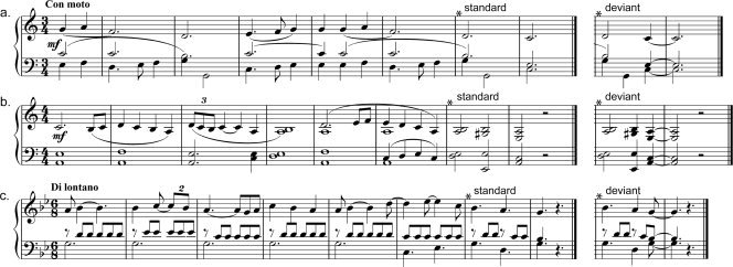
Examples of stimuli. Metrically standard and deviant endings for 3 (a–c) out of 30 different polyphonic piano compositions (composer Nicolaas Ravenstijn).

The metrically deviant stimuli described here were presented, interspersed in a within‐participants design, with the harmonically deviant stimuli described in James et al. [ 2008]. Thus, the actual trial sequence presented concurrently to the participants contained three experimental stimulus conditions: standard, metrically deviant, and harmonically incongruous versions of each composition. The harmonic incongruities consisted in imperfect but in‐key cadences. Metric and harmonic deviances were never combined. For full analysis of the responses to harmonically incongruent cadences, we refer to James et al. [ 2008]. The standard stimuli of both studies are thus identical data. In this study, our main analyses are focused on responses to metrically deviant endings compared with responses to standard endings.

The stimuli were executed by a professional pianist on an acoustical grand piano and recorded in stereo at 44,100 Hz, with a resolution of 16‐bit. Two independent professional musicians judged whether any effects revealed an upcoming incongruent ending, if such was the case, new recordings were made until no such effects were judged present. All terminal chords were cut off at 1,220 ms from onset and faded linearly over the last 70 ms. Mean intensity of the stimuli was 67.1 ± 1.4 dB (SD). Each stimulus was presented three times, resulting in 90 items for all three experimental conditions, with a total of 270 stimuli presentations. The stimuli were presented binaurally via headphones. All stimuli, conditions collapsed, were randomized and then divided into four blocks. The order of presentation within each of these four blocks was randomized again for each participant.

Behavioral Task

Participants were requested to indicate whether a musical piece provided a satisfactory ending by means of right hand button presses on a response box, using a button labelled with “NO” (middle finger) for not satisfactory endings, and with “YES” (index) for satisfactory endings. They were not informed on the three distinct categories of the stimuli. They were encouraged to respond naturally, and not to spend a lot of time on the decision. Participants were instructed to withhold their response until a prompt appeared on the screen (“please respond”), 1,720 ms after the onset of the terminal chord (duration of terminal chord plus 500 ms delay), to prevent contamination of the stimulus‐related EEG signal with motor activity. For that reason, only ratings of satisfactory ending but not reaction times are reported.

To compare responses to metrically standard and deviant cadences, we calculated the d‐prime or “sensitivity” score, based on Detection Theory [Macmillan and Creelman, 1997] and executed a one‐way ANOVA comparing d‐prime scores of experts and laymen.

EEG Acquisition and Raw Data Processing

EEG was continuously recorded from 128 electrode sites (BioSemi Active‐Two, V.O.F., Amsterdam, the Netherlands), equally distributed over the scalp. Data were digitized at a sampling rate of 1,024 Hz in a bandwidth filter of 0–268 Hz. Prior to analysis, data were offline recomputed against average reference, and band‐pass filtered (1–30 Hz). Averaged evoked potentials were calculated from stimulus onset (onset of the terminal chord of the piece) to 650 ms post stimulus. A DC shift correction was applied. In addition to an automated threshold rejection criterion of 50 μV, epochs were visually inspected for oculomotor and other artifacts using pre‐processing methods described in Michel and Brandeis [ 2009] and Brunet et al. [ 2011]. On average, 71.4 ± 8.9 epochs per condition per participant were retained.

Channels exhibiting substantial noise were interpolated using a 3D spherical spline interpolation that accounts for the real geometry of the head [Brunet et al., 2011; Perrin et al., 1989]. These interpolation methods have been successfully used in other publications using inverse solutions [Britz et al., 2009; Spierer et al., 2008] and are recommended for high density ERP source analysis [Brunet et al., 2011; Michel and Brandeis, 2009].

Procedure of ERP Analyses

Stage 1: ERP waveform analyses

In a 15 electrode site array divided in three zones, frontal (from left to right F3‐F1‐Fz‐F2‐F4), central (C3‐C1‐Cz‐C2‐C4), and parietal (P3‐P1‐Pz‐P2‐P4), ERPs and ERP difference waves (metrically deviant minus standard) were computed. Then mean voltage amplitudes over a 150–300 ms period from stimulus onset were calculated for all ERPs. This time period corresponds with the latency of early P3a responses to similar temporal transgressions [Jongsma et al., 2004; Vuust et al., 2009]. We conducted a repeated measures ANOVA on the mean amplitude of ERPs over this period (150–300 ms) with the factors Condition (2, within) × Zone (3, within) × Expertise (2, between).

Stage 2: Spatiotemporal ERP analyses (microstate segmentation)

ERP topographies do not randomly vary over time, but rather remain stable over periods of several tens of milliseconds, separated by abrupt changes [Brunet et al., 2011; Pascual‐Marqui et al., 1995]. These stable periods were conceptualized as microstates of information processing by Lehmann et al. [ 1987]. A k‐means cluster analysis allowed reducing our grand‐average ERP topographies over time into an optimal number of microstates or template maps, on the basis of cross validation criteria, that minimize the residual variance, and the Krzanowski‐Lai criterion [Brunet et al., 2011; Michel and Brandeis, 2009; Michel et al., 2004; Murray et al., 2008; Pascual‐Marqui et al., 1995]. The resulting microstate series can be considered an a priori hypothesis that has to be statistically tested. Therefore spatial correlation coefficients were computed time‐point wise between the microstates or ERP template maps identified by the cluster analysis in the grand‐average ERPs and the ERPs of each participant for each condition. This yields measures of map presence or “map duration” (expressed in ms) for each participant and condition that can be submitted to statistical testing, thus “fitting” the microstates to the actual data. We conducted a repeated measures ANOVA on map duration with the factors Condition (2, within) × Map configuration (number of microstates, within) x Expertise (2, between). We also examined effects for duration of these maps for each group separately, via repeated measures ANOVAs with the factors Condition (2, within) × Map configuration (number of microstates, within). Finally, we performed an analysis on latency or onset, another parameter resulting from the spatiotemporal analysis, for a late positive microstate, marking the end of processing in all groups in our window of analysis.

Stage 3: Statistical analyses of ERP sources

Only when the spatial configuration of the electric field at the scalp level differs, different underlying neuronal populations can be assumed, reflecting an alteration of the functional state of the brain [Michel et al., 1999a, b]. We therefore based our ERP source analysis on the results of the spatiotemporal ERP analyses.

First we compared statistically putative underlying sources over periods during which an identical microstate map occurred simultaneously in both groups with different strength, namely for the early P3a‐like component or microstate 3 (see Results section). Then we compared sources over consecutive periods during which different maps occurred simultaneously, thus evaluating differences in the configuration of intracranial generators.

A depth‐weighted minimum norm distributed linear inverse solution [Hamalainen and Ilmoniemi, 1994; Michel et al., 2004] was computed to estimate the intracranial current distribution (current density in μA/mm³) at each moment in time for the evoked potential of each participant. The current distribution was calculated within the gray matter of the average brain provided by the Montreal Neurological Institute. A discrete grid of 3,005 solution points was regularly distributed within the gray matter of this MRI. After applying a homogenous transformation operation to the volume that rendered it to the best fitting sphere [Spinelli et al., 2000], a 3‐shell spherical head model was used to calculate the lead field for the 128 electrodes. The solution space was then spatially smoothed by averaging the solution points within 25 Regions of Interest (ROIs) in each hemisphere [50 in total; the same as in James et al., 2008; see Table I], conform to the Automated Anatomical Labeling [AAL; Rorden and Brett, 2000; Tzourio‐Mazoyer et al., 2002]. Because our source estimations derive from ERP results, our source points were confined to cortical and limbic gray matter.

Table I.

ROI list

LOBE	ROI	Number
Frontal	Left Superior Frontal Cortex	1
	Right Superior Frontal Cortex	2
	Left Orbitofrontal Cortex	3
	Right Orbitofrontal Cortex	4
	Left Middle Frontal Cortex	5
	Right Middle Frontal Cortex	6
	Left Inferior Frontal Cortex	7
	Right Inferior Frontal Cortex	8
	Left Supplementary Motor Area	9
	Right Supplementary Motor Area	10
	Left Insula	11
	Right Insula	12
	Left Anterior Cingulate Cortex	13
	Right Anterior Cingulate Cortex	14
Parietal	Left Superior Parietal Cortex	15
	Right Superior Parietal Cortex	16
	Left Inferior Parietal Cortex	17
	Right Inferior Parietal Cortex	18
	Left Precuneus	19
	Right Precuneus	20
	Left Middle Cingulate Cortex	21
	Right Middle Cingulate Cortex	22
	Left Posterior Cingulate Cortex	23
	Right Posterior Cingulate Cortex	24
Temporal	Left Superior Temporal Cortex	25
	Right Superior Temporal Cortex	26
	Left Middle Temporal Cortex	27
	Right Middle Temporal Cortex	28
	Left Inferior Temporal Cortex	29
	Right Inferior Temporal Cortex	30
	Left Fusiform Gyrus	31
	Right Fusiform Gyrus	32
	Left Heschl's Gyrus	33
	Right Heschl's Gyrus	34
	Left Temporal Pole	35
	Right Temporal Pole	36
	Left Hippocampal complex	37
	Right Hippocampal complex	38
	Left Amygdala	39
	Right Amygdala	40
Occipital	Left Calcarine Sulcus	41
	Right Calcarine Sulcus	42
	Left Lingual Gyrus	43
	Right Lingual Gyrus	44
	Left Superior Occipital Cortex	45
	Right Superior Occipital Cortex	46
	Left Middle Occipital Cortex	47
	Right Middle Occipital Cortex	48
	Left Inferior Occipital Cortex	49
	Right Inferior Occipital Cortex	50

ROIs defined according to the Automated Anatomical Labeling [AAL; Rorden and Brett, 2000; Tzourio‐Mazoyer et al., 2002].

First, we averaged the current density values (μA/mm³)—for each individual and each ROI—within 4 consecutive time periods between 150 and 650 ms. The choice of these time periods derived from the spatiotemporal ERP analyses.

Then we computed “omnibus” repeated ANOVAs with the factors Condition (2, within) × Hemisphere (2, within) × ROI (25, within) × Expertise (2, between) for each time period. These omnibus ANOVAs also allowed verifying our a priori hypotheses by visual inspection. Consecutively, to verify our a priori hypotheses, we carried out separate repeated measures ANOVAs with the design Condition (2, within) × Hemisphere (2, within) × Expertise (2, between) for 8 particular ROIs in each hemisphere (16 in total), for each of the 4 time periods. These 8 ROIs pertained to three different categories according to our a priori hypotheses. The first category included ROIs associated with actual and imaginary musical motor performance and meter perception, for which we expected stronger activation in experts in response to metric deviance, that is, SMA (BA 6), middle and posterior cingulate cortex (BA 31) and precuneus (BA 7) [Bengtsson et al., 2009; Langheim et al., 2002; Lotze et al., 2003; Parsons, 2001; Parsons et al., 2005]. The second category of ROIs was associated with visual imagery, expected to be recruited also more strongly in experts during music processing, that is, the superior occipital cortex [encompassing part of the cuneus, i.e., BA 19; Bengtsson et al., 2009; Meister et al., 2004; Schmithorst and Holland, 2003]. Finally, we examined three ROIs in the medial temporal lobe, known to be involved in harmony incongruity processing in experts [James et al., 2008], that is, hippocampal complex, amygdala and insula (BA 13). One could argue that the analysis of potentials in amygdala and hippocampus is problematic due to the cytoarchitectonics of these structures. However, studies using simultaneous or alternated recordings of intracranial and scalp EEG have shown that medial‐temporal activity can be reliably retrieved from scalp EEG, using distributed source reconstruction techniques similar to those used in this study [James et al., 2009; Lantz et al., 1997; Nahum et al., 2010; Zumsteg et al., 2005].

RESULTS

First we verified all datasets for normal distribution (Kolmogorov‐Smirnov statistic, P < 0.05). Then error probability was corrected according to Greenhouse and Geisser [ 1959] to compensate for nonsphericity; adjusted P‐values and degrees of freedom are reported.

Behavioral Results

Experts judged 96.3 ± 2.2% (SD) of the metrically standard cadences as “satisfactory” (“YES”) versus 80.7 ± 16.2% for the laymen. In response to metrically deviant cadences, experts judged 56.1 ± 33.4% of the stimuli as “unsatisfactory” (“NO”) versus 36.1 ± 17.2% for the laymen. A one‐way ANOVA on d‐prime scores evidenced significantly higher values for experts (2.08 ± 1.22) than for laymen (0.63 ± 0.24; F _{1, 24} = 17.8; P < 0.0003), indicating that experts were more sensitive to metric deviance.

Results of EEG Analyses

Stage 1: ERP waveform analyses

Visual inspection of grand‐average ERP waveforms for experts and laymen confirmed the occurrence of an early P3a‐like component [Jongsma et al., 2004; Vuust et al., 2009] at 150–300 ms after stimulus presentation. This component occurred in both conditions and groups, but its amplitude in experts was enhanced in response to metric deviance compared to regular endings; for laymen its amplitude was reduced (Fig. 2a–c, mean topographic voltage maps (150–300 ms) are depicted in Fig. 2d).

Figure 2.

Figure 2. Grand‐average ERP waveforms for an array of 15 electrode sites. ERPs in response to (a) metrically standard endings, (b) metrically deviant endings, and (c) difference ERPs between conditions (deviant minus standard), plotted for Experts (in red) and Laymen (in black). Gray shaded areas show the time interval used for the statistical analysis of the ERPs (150–300 ms). Topographic scalp configurations (d) are shown for each group and each condition (S: standard; D: deviant) and for difference ERPs (D‐S: deviant minus standard), depicting the average voltage over the 150–300 ms time period at all 128 electrode sites. These maps are 2‐D projections of the 3‐D electrode configuration (view from above, nasion on top). (e) Left panel: highlighted head positions of the 15 electrodes within the array depicted in gray amongst all other electrode sites (total n = 128), right panel: enlarged labeled array.

We verified these observations via a repeated measures ANOVA on the mean amplitude (150–300 ms) of the ERPs within the defined 15‐electrode array (Fig. 2e), with the factors Condition (2, within) × Zone (3, within) × Expertise (2, between). A main effect of Expertise (F _{1, 24} = 9.1, P < 0.006) indicated that ERP responses of experts gave rise to higher amplitudes in response to all musical stimuli. A main effect of Zone (F _{1.2, 28.2} = 36.9, P < 0.0001) reflected the P3a‐like amplitude configuration, with positive values in the frontal and central zones and negative ones in the parietal zone, for both groups. Critically, triple interaction Condition × Zone × Expertise (F _{1.4, 33.8} = 37.0, P < 0.0001) demonstrated that experts displayed more positive amplitudes in the frontal zone in response to meter deviance as compared with standard endings, whereas laymen showed less positive ones. Moreover, in the parietal zone, the reversed pattern occurred: experts exhibited lower amplitudes, resulting in negative values and laymen more positive amplitudes in response to deviance as compared with standard endings.

To check whether responses to deviant versus standard cadences were different for each group within this 15‐electrode array, we also ran ANOVAs for each group separately with the design Condition (2, within) × Zone (3, within). Condition × Zone interaction was significant for experts (F _{1.5, 17.5} = 26.4, P < 0.0001) with higher amplitudes in the frontal zone and lower ones in the parietal zone in response to deviant cadences. For the laymen, this interaction was also significant (F _{1.3, 16.1} = 11.2, P < 0.002), but showed an opposite pattern with lower values in the frontal zone and higher ones in the parietal zone in response to deviance.

For illustration purposes, Figure 2c also depicts the ERP difference waves (metrically deviant minus standard). These data highlight that experts exhibited larger differences between ERP responses to deviant versus standard endings than laymen.

Correlation d‐prime and P3a

To verify the correlation between d‐prime scores and the P3a‐like component we performed a simple regression analysis with d‐prime scores as continuous predictor on mean amplitude (150–300 ms) of difference waves (metrically deviant minus standard) in the frontal zone of the 15‐electrode array (cf. Fig. 2c), where this component manifests most typically [Polich and Criado, 2006]. We chose difference waves because, like the d‐prime score, they reflect a relationship between responses to deviant and standard endings. This regression turned out positive (β = 0.62 ± 0.16) and highly significant (t = 3.9; P < 0.0007). So higher d‐prime scores, or higher sensitivity to metrical deviance, resulted in higher amplitudes of difference waves for this component.

Stage 2: Spatiotemporal ERP analyses (microstate segmentation)

The spatiotemporal segmentation procedure identified seven distinct ERP template maps (or microstates), which explained ∼85% of the variance in both conditions and groups during the time period 0–650 ms. Mean onset and duration of these microstates are illustrated in Figure 3a; the corresponding scalp voltage configurations can be visualized in Figure 3b.

Figure 3.

Results of spatiotemporal ERP analyses. (a) A k‐means clustering analysis yielded 7 distinct microstate maps that optimally represent the data of both groups and both conditions (E: Experts, L: Laymen, std: metrically standard ending, dev: metrically deviant ending). The segments under the GFP curves represent the time periods during which each of these microstate maps was most represented in the group data. The segments are marked in black and gray when common to both groups, and in color when unique for one group or one condition at a certain time period. The average onset and offset of each microstate are indicated in ms. (b) Scalp configurations of the microstate maps, framed in corresponding color‐code; positive voltages in red, negative in blue. These maps are 2‐D projections of the 3‐D electrode configuration (view from above, nasion on top). (c) Mean duration of microstate maps resulting from individual subject fitting for both experimental groups and conditions for two consecutive time periods. Vertical bars depict 95% confidence intervals.

In an initial period (∼0−250 ms), for both conditions and groups, three maps (# 1, 2, and 3) arose successively in similar order: 1‐2‐1‐3. Map 3 gave rise to strong amplitudes, peaked shortly before 200 ms, and marked the end of commonality of processing between conditions and groups. This map corresponds in timing and topography to the early P3a‐like component as delineated by the preceding waveform analyses (cf. Fig. 2). In the period preceding this P3a‐like component, no statistically significant differences in duration or appearance of microstate maps were found between groups and conditions.

Repeated measures ANOVAS were then computed on microstate map duration (in ms) for two periods during which different maps occurred at the same time in both groups, 250–400 ms and 400–650 ms (Fig. 3c1,2).

For the period of 250–400 ms after stimulus onset (encompassing 4 maps: # 2, 4, 5, and 6; Fig. 3c1), we executed an ANOVA with the factors Condition (2, within) × Map configuration (4 maps: 2, 4, 5, and 6, within) × Expertise (2, between) on map duration (in ms). Two significant results emerged. First, Map configuration × Expertise interaction (F _{2.5, 60.6} = 4.7, P < 0.008) showed that map 6 (cf. Fig. 3b) was more present in laymen across both conditions compared to experts (cf. Fig. 3a,c1); inversely map 5 was more present in experts. Second, Condition × Map configuration interaction (F _{2.5, 60.7} = 3.9, P = 0.018) showed a longer duration of map 2 for deviant endings and, to a lesser extent, a longer duration of map 4 for standard endings (Fig. 3c1). We presumed that the expert group caused this observation. To verify this presumption, we computed additional ANOVAs with the factors Condition (2, within) × Map configuration (4 maps: 2, 4, 5, and 6, within) for each group separately. Condition × Map configuration interaction was significant for experts (F _{2.5, 29.6} = 7.0 P < 0.002), but not for laymen. In the latter group, map duration was more or less stable across conditions. In contrast, as presumed, experts showed longer duration in response to metric deviance for map 2, and longer duration in response to standard closure for map 4. Hence, microstate or map 2 (cf, Fig, 3b) characterized expert processing of metric deviance in this time period.

For the final time period of 400–650 ms (encompassing 3 maps: # 4, 6, and 7, Fig. 3c2), a similar ANOVA was performed on durations with the factors Condition (2, within) × Map configuration (3, within) × Expertise (2, between). A main effect of Map configuration arose (F _{1.9, 45.9} = 13.5, P < 0.0001), demonstrating longer durations of map 4 (cf. Fig. 3b) compared with the other 2 maps. Interaction Map configuration × Expertise (F _{1.9, 45.9} = 9.0, P < 0.001) revealed that experts spent more time in the microstate of map 4 relative to laymen. Furthermore, triple interaction Condition × Map configuration × Expertise (F _{2.0, 46.8} = 8.2, P < 0.001) showed that experts exhibited the longest durations for map 4 in response to meter deviance, whereas laymen spent less time in microstate 4 in response to deviance as compared with standard endings.

Next, in order to investigate processing speed, we applied a repeated measures ANOVA on mean onset (in ms) or latency of microstate 4 over the final time period (400–650 ms) with the factors Condition (2, within) × Expertise (2, between). This map constitutes the final microstate for all conditions and groups in our time period of analysis. A main effect of Expertise (F _{1, 24} = 6.0, P = 0.022) as well as Condition × Expertise interaction reached significance (F _{1, 24} = 8.1, P < 0.009). First onset of this microstate map occurred ∼ 80 ms earlier in experts than in laymen in response to metric deviance.

Deviance detection

In principle, separate ERP analyses on correct responses or “hits” (“NO” responses) for metrically deviant endings were limited due to insufficient epochs per condition per individual. However, we did perform such an exploratory analysis for the laymen, who produced low sensitivity scores, to compare correct identifications of deviant endings with the averaged responses for hits and misses. A spatiotemporal ERP analysis comparing ERPs of hits versus ERP responses to all deviant endings for the laymen group did not yield any statistically significant differences: the microstate maps explaining the data were identical. This was also found for ERPs in response to harmonically inappropriate endings [James et al., 2008].

Stage 3: Statistical analyses of ERP sources

Based on the results of our spatiotemporal ERP analyses, we determined four time periods during which either an identical ERP map (microstate) occurred simultaneously in both groups with different strength (Period 1, 143–261 ms), or different maps occurred during the same interval (Period 2, 270–361 ms; Period 3, 395–457 ms; Period 4, 469–610 ms; cf. Fig. 3a).

We then estimated intracranial ERP sources by computing mean current density values (μA/mm³) in all 50 ROIs (25 in each hemisphere) for each participant and condition over each time period. Omnibus repeated measures ANOVAs with the factors Condition (2, within) × Hemisphere (2, within) × ROI (25, within) × Expertise (2, between) were computed. Results are summarized in Table II, and further detailed below for each time period.

Table II.

ANOVAs on ERP brain sources

Time Period	143–261 ms		270–361 ms		395–457 ms		469–610 ms
Effect	df	F‐value	df	F‐value	df	F‐value	df	F‐value
EX	1, 24	6.6*	1, 24	1.9	1, 24	1.8	1, 24	1.3
CO	1, 24	<1	1, 24	1.6	1, 24	2.5	1, 24	2.0
CO × EX	1, 24	6.0*	1, 24	<1	1, 24	<1	1, 24	<1
HP	1, 24	6.2*	1, 24	2.8	1, 24	5.9*	1, 24	2.3
HP × EX	1, 24	3.8	1, 24	<1	1, 24	<1	1, 24	<1
ROI+	3.5,83.0	40.1****	2.8, 68.0	54.4****	3.8, 92.0	55.0****	4.3, 102.3	56.2****
ROI × EX+	3.5,83.0	1.9	2.8, 68.0	1.3	3.8, 92.0	1.6	4.3, 102.3	<1
CO × HP	1, 24	<1	1, 24	<1	1, 24	4.5*	1, 24	1.8
CO × HP × EX	1, 24	1.7	1, 24	<1	1, 24	<1	1, 24	3.4
CO × ROI+	4.0, 95.7	<1	5.3, 127.3	1.1	4.5, 106.9	<1	4.6, 110.9	<1
CO × ROI × EX+	4.0, 95.7	1.4	5.3, 127.3	1.5	4.5, 106.9	2.0	4.6, 110.9	2.2°
HP × ROI+	5.0, 120.8	20.0****	3.9, 94.0	9.8****	4.3, 103.5	9.6****	4.7, 113.4	14.4****
HP × ROI × EX+	5.0, 120.8	1.4	3.9, 94.0	<1	4.3, 103.5	1.1	4.7, 113.4	<1
CO × HP × ROI+	5.9, 141.8	<1	4.3, 103.5	<1	5.6, 134.7	1.9	5.7, 136.8	1.4
CO × HP × ROI × EX+	5.9, 141.8	<1	4.3, 103.5	<1	5.6, 134.7	1.2	5.7, 136.8	1.6

°P < 0.07 *P < 0.05, **P < 0.01, ***P < 0.001, ****P < 0.0001, ⁺Greenhouse‐Geisser adjusted.

F values and significance levels for omnibus ANOVAs on ERP brain sources for effects of Expertise (EX), Condition (CO), Hemisphere (HP), and all 50 Regions of Interest (ROI; 25 in each hemisphere) within 4 consecutive time periods based on the outcome of the spatiotemporal ERP analyses.

Consecutively, repeated measures ANOVAs on mean current density were executed for eight particular ROIs, selected on the basis of prior imaging work, defined in the Methods Section (Stage 3: Statistical analyses of ERP sources). These ANOVAs were executed for each of these ROIs separately with the factors Condition (2, within) × Hemisphere (2, within) × Expertise (2, between). Results are summarized in Table III, and further detailed below for each time period. In the following Results section, we will only report on significant effects of Expertise and Condition and their interactions.

Table III.

ANOVAs on 8 a priori ROIs

Effect		F‐values
ROI	df	SMA	INS	PRECUN	mCING	pCING	HIP	AMYG	sOCC
Time period 1: 143–261 ms
EX	1, 24	7.6*	5.9*	6.6*	7.7**	7.4*	3.4	3.8	7.0*
CO	1, 24	<1	<1	1.2	<1	<1	<1	<1	2.6
CO × EX	1, 24	7.0*	1.9	7.3*	8.5**	13.8***	1.3	<1	2.6
HP	1, 24	3.7	12.3**	12.0**	25.2****	10.4**	<1	1.0	12.3**
HP × EX	1, 24	<1	6.1*	5.0*	<1	1.6	3.6	7.0*	7.4*
CO × HP	1, 24	<1	<1	<1	<1	<1	<1	<1	1.8
CO × HP × EX	1, 24	5.0*	<1	<1	5.2*	<1	<1	<1	<1
Time period 2: 270–361 ms
EX	1, 24	3.8	0.6	2.1	3.1	2.5	4.0	2.9	3.0
CO	1, 24	3.9	4.8*	<1	2.1	1.5	<1	1.6	<1
CO × EX	1, 24	6.4*	<1	1.5	<1	<1	<1	<1	<1
HP	1, 24	0.4	3.8	22.3****	1.3	<1	<1	<1	4.1
HP × EX	1, 24	5.5*	<1	<1	<1	<1	<1	<1	<1
CO × HP	1, 24	2.0	<1	<1	<1	<1	1.1	<1	1.1
CO × HP × EX	1, 24	0.1	2.8	<1	<1	<1	4.3*	7.7*	<1
Time period 3: 395–457 ms
EX	1, 24	4.0	<1	2.9	2.5	2.4	<1	<1	6.3*
CO	1, 24	<1	1.0	4.1	<1	1.4	<1	<1	3.1
CO × EX	1, 24	<1	<1	2.7	<1	<1	1.7	1.2	7.0*
HP	1, 24	1.4	13.0**	19.6***	<1	<1	<1	3.6	7.7*
HP × EX	1, 24	<1	<1	<1	2.3	1.6	<1	<1	<1
CO × HP	1, 24	1.2	<1	<1	1.5	<1	1.6	<1	<1
CO × HP × EX	1, 24	<1	1.8	1.7	<1	<1	<1	<1	<1
Time period 4: 469–610 ms
EX	1,24	3.1	<1	3.1	5.8*	7.6*	1.9	1.7	2.3
CO	1,24	<1	<1	2.3	2.6	3.1	<1	<1	2.7
CO × EX	1,24	<1	<1	4.2*	1.6	3.4	<1	<1	1.3
HP	1,24	2.3	7.9**	13.5**	5.8*	<1	2.0	2.1	21.8****
HP × EX	1,24	<1	<1	<1	<1	<1	<1	2.5	<1
CO × HP	1,24	<1	<1	<1	<1	6.6*	2.9	<1	<1
CO × HP × EX	1,24	<1	7.0*	3.4	<1	6.6*	3.3	6.5*	3.1

*P < 0.05, **P < 0.01, ***P < 0.001, ****P < 0.0001.

SMA, supplementary motor area; INS, insula; PRECUN, precuneus; mCING, middle cingulate cortex; pCING, posterior cingulate cortex; HIP, hippocampus; AMYG, amygdala; sOCC, superior occipital cortex.

F values and significance levels for ANOVAs on 8 ROIs, based on a priori hypotheses, for effects of Expertise (EX), Condition (CO), and Hemisphere (HP), within 4 time periods deriving from the spatiotemporal ERP analyses.

Time Period 1 (143–261 ms)

This time period yielded the strongest differences between groups and conditions. The omnibus ANOVA (Table II, columns 1 and 2; Fig. 4a) gave rise to a main effect of Expertise, experts responded with higher brain activity than laymen to all musical stimuli. Condition × Expertise interaction demonstrated that brain activation differences between experts and laymen were stronger in response to metrically deviant cadences than to standard closure.

Figure 4.

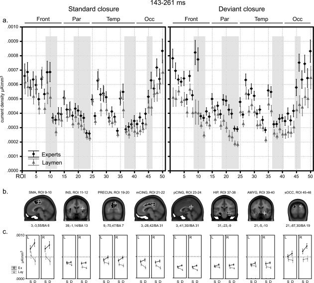
Results of statistical source analyses of ERPs; time‐period 143–261 ms. (a) Mean current density values (μA/mm³) for all 50 ROIs (cf. Table I) of both experimental groups and conditions for the 143–261 ms time period resulting from the spatiotemporal ERP analyses. On top of the graphs a division of ROIs in frontal (Front), parietal (Par), temporal (Temp), and occipital (Occ) lobes is provided. Vertical bars depict standard errors. Gray‐shaded areas highlight values for the 8 predefined ROIs. (b) The 8 predefined ROIs are highlighted, superimposed on MNI 152 template brain slides. Talairach coordinates are provided underneath, corresponding to the position of the superimposed white cross. Corresponding Brodmann areas (BA) are provided when available. (c) Below each ROI mean current density values for both groups (Ex: experts, in black; Lay: laymen in gray) and both conditions (S: standard endings, D: deviant endings) are depicted for each cerebral hemisphere (L: left, R: right). Vertical bars depict standard errors. For significant differences, we refer to Table III, top panel (Time period 1: 143–261 ms).

The ANOVAs on 8 a priori defined ROIs (Table III, top panel; Fig. 4b,c), revealed a main effect of Expertise in the SMA, insula, middle and posterior cingulate, precuneus, and superior occipital areas where experts exhibited higher current density than laymen in response to all musical stimuli. No such effect of Expertise manifested in the hippocampal complex or amygdala. More interestingly, Condition × Expertise interaction reached significance in the SMA, middle and posterior cingulate and precuneus. In these areas, metric deviance at closure evoked stronger activation than standard endings in experts, whereas laymen showed reduced activations. Moreover, supplementary motor and middle cingulate activations also gave rise to significant triple interaction of Condition × Hemisphere × Expertise. In these two areas, metric deviance induced higher activations in experts but lower activations in laymen, relative to standard stimuli, and more strongly so in the left hemisphere. Hence, modest left hemisphere dominance occurred in experts for these effects in SMA and middle cingulate cortex. Interaction of Hemisphere × Expertise manifested in the precuneus, insula, and amygdala, where laymen displayed a slight left dominance and also in the superior occipital cortex where experts showed a marked right dominance.

To compare these data with our previous findings of early enhanced responses to harmonic incongruence in the right hippocampal complex, amygdala and insula for experts but not laymen [James et al., 2008], we also computed direct contrasts between groups for metric deviance effects in these areas. In right amygdala and insula, experts showed stronger responses to metric deviance compared with laymen (respectively F _{1, 24} = 9.8, P < 0.005; F _{1, 24} = 16.4, P < 0.001), but not in the hippocampal complex. However, Condition × Expertise interaction did not reach significance in these medial temporal areas unlike in the SMA, middle and posterior cingulate, and precuneus (see Fig. 4b,c; Table III, top panel).

Time Period 2 (270–361 ms)

The omnibus ANOVA (Table II, columns 3 and 4) did not yield any significant effects related to Expertise or Condition. The ANOVAs on 8 a priori defined ROIs (Table III, second panel) did not produce any main effects of Expertise. A main effect of Condition arose in the insula, with stronger responses to deviance than to standard cadences in both groups. In the SMA, Condition × Expertise interaction occurred again; experts exhibited stronger responses to deviance relative to standard stimuli, and laymen weaker ones. Hemisphere × Expertise interaction also manifested in the SMA, with stronger right activations for experts. Finally, triple interaction Condition × Hemisphere × Expertise in the hippocampal complex and amygdala showed slightly larger differences between experimental groups in response to deviance in the right hemisphere, due to amplified values for experts. Contrasts between groups in response to deviance in the right hemisphere of these two ROIs did not yield significant results (cf. time period 1).

Time Period 3 (395–457 ms)

The omnibus ANOVA (Table II, columns 5 and 6) did not yield significant effects of Expertise. Condition × Hemisphere interaction revealed that in this time period, no differences between conditions (collapsed across all ROIs) occurred in the left hemisphere, whereas in the right hemisphere, deviant stimuli yielded stronger activations than standard ones.

The ANOVAs on 8 a priori defined ROIs (Table III, third panel), yielded a main effect of Expertise for the superior occipital cortex. Condition × Expertise interaction was also significant in this area: experts showed stronger activations in response to deviance compared with standard stimuli; laymen did not show different responses as a function of condition.

Time Period 4 (469–610 ms)

The omnibus ANOVA (Table II, columns 7 and 8) gave rise to marginally significant triple interaction Condition × ROI × Expertise (F _{10.6, 110.9} = 2.2, P = 0.068). Stronger responses to deviance could be observed in the precuneus and cingulate cortices in experts as compared with laymen (left and right hemisphere collapsed). These observations are confirmed in the following section.

The ANOVAs on 8 a priori (Table III, bottom panel) defined ROIs yielded main effects of Expertise in the middle and posterior cingulate cortices, where experts showed increased activity in all conditions. Condition × Expertise interaction was significant in the precuneus, where experts exhibited stronger activation in response to deviance relative to standard endings, versus laymen reduced responses. Triple Condition × Hemisphere × Expertise interaction occurred in the posterior cingulate cortex, as well as in the insula and amygdala. In the posterior cingulate cortex, the increased response of experts to deviance was the strongest in the left hemisphere, whereas laymen showed weak uniform responses in both conditions and hemispheres. For the insula and amygdala, responses were increased in experts relative to laymen; these differences were stronger in the right hemisphere for standards and in the left hemisphere for deviants.

Supplementary Results, Statistical Parametric Mapping of Estimated Sources Over Time

To ensure that the here found early enhanced motor activations in experts are specific for the processing of meter deviance with respect to harmonic deviance processing, we submitted both data sets to an identical analysis over time as in James et al. [ 2008]. Unpaired t‐tests (two‐tailed) between musical experts and laymen were computed for the 50 ROIs on current density (μA/mm³) in response to both metric and harmonic deviance over 300 ms from stimulus onset. Applying identical criteria as in James et al. [ 2008], only periods for which this test exceeded a 0.005 alpha criterion for at least 40 consecutive ms were retained. The early enhanced expert responses in bilateral SMA (ROI 9 and 10, Table I) reported here only appeared in response to metric deviance and not in response to harmonic deviance (Fig. 5). For more detailed information on the responses to harmonic deviance and the statistics used, we refer to James et al. [ 2008].

Figure 5.

Statistical parametric mapping (SPM) of estimated sources, comparing experts and laymen for metric and harmonic deviance processing over 300 ms from stimulus onset. Results are shown within 50 Regions of interest (ROI, on the y‐axis; Table 1) estimated by a distributed linear inverse solution (WMN). Time course of current density differences between experts and laymen is shown in graduated light‐gray shades for metric deviance and in graduated dark‐gray shades for harmonic deviance (James et al., 2008). The shaded areas indicate when current density significantly differed between the two groups for more than 40 ms; significant p‐values vary from P < 0.005 (darkest shades) up to P < 0.0001 (lightest shades). Vertical bars depict 95% confidence intervals. For metric deviance significant differences occurred in bilateral SMA (ROIs 9 & 10); for harmonic incongruity significant differences occurred in right hippocampal complex, amygdala and insula (respectively ROIs 38, 40 and 12). In both cases the enhanced responses occurred in the expert group. (Adapted with permission from James CE et al. 2008, 42:1597–1608, Elsevier).

DISCUSSION

The cardinal result of this study is that subtle transgressions of metric expectancies at musical closure elicited an enhancement of an early P3a‐like response in professional pianists versus a reduction in laymen, relative to the response evoked by metrically standard endings. These electrophysiological results were highly correlated to the sensitivity scores for metrical deviance. Putative contributive sources for these ERP modulations were localized within bilateral motor and premotor regions (such as SMA and mid/post‐cingulate), as well as in areas associated with self‐referential processing and mental imagery (such as precuneus and extrastriate cortex) and relevance detection (right amygdala). The modulation of this P3a‐like component and its associated sources in experts may reflect a stronger “embodiment” of rhythmic expectation in musicians relative to laymen. In contrast, the laymen's reduced responses to metrical deviance may imply a disruption of “sensorimotor resonance” provoked by the metric anomalies.

In the following Discussion section, we will mainly focus on the critical Condition × Expertise interaction.

Early Processing (∼0–250 ms)

The P3a‐like waveform, associated with microstate 3 identified by the spatiotemporal ERP analysis (onset ∼ 150 ms, peak ∼ 200 ms), arose in response to both standard and deviant cadences in both groups. The association between the P3a‐like component and microstate 3 is based on the similar timing and scalp topography (cf. Fig. 2, bottom panel and Fig. 3b). Conventional ERP analyses and spatiotemporal ERP analyses of the same data logically yield partially overlapping information. ERP components and microstates may envelop each other. The ERP amplitude analyses (Fig. 2) were slightly more extended over time (150–300 ms) to allow comparisons to the literature [Jongsma et al., 2004; Vuust et al., 2009].

Transgression of musical expectancy can affect the amplitude of P3a responses in various conditions, including harmony violation [Carrion and Bly, 2008; Regnault et al., 2001] and metric transgression [Jongsma et al., 2004; Vuust et al., 2009]. In agreement with Vuust et al. [ 2009], we would argue that the modulations of the P3a‐like activity found here may primarily represent an index of temporal expectation, rather than the P3a typically found in oddball paradigms [Polich and Criado, 2006]. Increased amplitude of this P3a in experts therefore suggests enhanced expectations due to musical rhythmical experience and training, and converges with the correlated behavioral results showing higher d‐prime values and thus greater sensitivity to metric deviance in experts.

According to the source estimations, brain areas contributing to the modulation of this P3a‐like component resided in a network comprising bilateral SMA (medial premotor/BA 6), plus middle and posterior cingulate cortex (BA 31) and precuneus (BA 7). In all these regions, stronger activations occurred in response to metrically deviant endings compared with standard ones in experts, whereas weaker activations arose in laymen. The argument that these sources reflect the Condition x Expertise interaction observed at the scalp level supports our assumption that these areas contribute to the modulation of the ERPs.

Several studies [Limb et al., 2006; Vuust et al., 2005, 2009] reported enhanced brain responses in the left hemisphere to metric incongruities in expert musicians compared to nonmusicians. In this experiment, we did not find any hemispheric differences in the conventional ERP analyses (Fig. 2e). An explanation may reside in the fact that the mentioned studies presented rhythm patterns, not full musical excerpts like here, to the participants. However, a moderate left hemisphere dominance expressed in experts in SMA and middle cingulate cortex during early processing.

The SMA is involved in planning, preparation, execution, and control of bimanual sequential finger movements. A positive correlation between gray matter and musician status has been shown in this medial premotor area in keyboard players [Gaser and Schlaug, 2003]. In this study, the explicit SMA activations suggest a recruitment of motor regions, in keeping with enhanced audio‐motor coupling in expert instrumentalists [Baumann et al., 2007; Haueisen and Knosche, 2001; Zatorre et al., 2007]. Such coupling may transform musical auditory inputs into temporally organized motor patterns. Therefore, the modulation of SMA activation patterns induced by metrical deviance may reflect a specific role in temporal sensory prediction for this brain area [Bengtsson et al., 2009; Grahn and Rowe, 2009].

In addition to the SMA, part of the middle cingulate cortex also carries out premotor functions [Vogt and Laureys, 2005]. Moreover, processing of various components of rhythm (pattern, tempo, meter, and duration) consistently engaged the cingulate cortex [Parsons, 2001]. Functional neuroimaging in pianists demonstrated that performing scales activated the middle and posterior cingulate cortex (BA 31) and the right precuneus more strongly than performing a learned musical piece of Bach [Parsons et al., 2005]. Because performing scales represents a relatively mechanical, purely motor aspect of piano playing, these data would be consistent with a motor role for these cingulate regions in relation to regular or rhythmic motor patterns. In the same study [Parsons et al., 2005], the opposite comparison showed that performing the Bach piece engaged the SMA, cuneus and insula more strongly than playing scales, thus suggesting a specific role in higher order music processing for these brain areas. The cuneus can also show a specific sensitivity to metric deviance [Bengtsson et al., 2009]; this area partly overlaps with the extrastriate superior occipital cortex (BA 19), where enhanced activations were observed in the experts in our study in early and later processing.

A concern might arise concerning possible motor contamination of brain responses as a consequence of motor preparation for the button presses. However, the results from the source analyses consisted in SPMs (statistical parametric mappings) that contrasted experts and laymen for both conditions via repeated measures ANOVAs. Consequently, covert or overt motor responses common to both groups were cancelled out and only significant differential activations reported. Thus both SMA and cingulate activations in response to deviant endings were enhanced in experts relative to laymen, compared to standard closure (Fig. 4c), irrespective of button presses. Moreover, several publications on music perception, using paradigms without any overt motor responses, also reported SMA activation, and stronger so in trained musicians than in naive listeners [Baumann et al., 2007; Bengtsson et al., 2009; Langheim et al., 2002; Zatorre et al., 2007].

Later Processing (∼250–650 ms)

In a subsequent period of 250–400 ms post‐stimulus, a single microstate (map 6, cf. Fig. 3b), with weak amplitude, manifested predominantly in laymen, in response to all musical stimuli. During the same time period, another microstate (map 2) expressed more strongly in experts in response to metric deviance. In the corresponding interval of 270–361 ms during which these two maps overlapped (microstate 2 in experts and microstate 6 in laymen, cf. Fig. 3a,b), the source estimations revealed that the SMA showed again stronger activations in experts, converging with the idea that the SMA may play a key role in the differential processing of metric deviance in experts, as discussed above.

In the final time period of 400–650 ms post‐stimulus, another distinctive microstate (map 4, cf. Fig. 3b), expressed prominently in experts, occurring stronger and earlier in response to metric deviance compared with laymen. This is in line with recent observations [Marie et al., 2011] of an enhanced late positivity/P600 component in musicians as compared with nonmusicians in relationship with a decision task on metric congruity in both language and music. Such a late positivity may reflect a top‐down capacity of applying a phrasing concept that is more precisely stored as a function of expertise [Bigand et al., 2005; Neuhaus et al., 2006], at this point in time at a more conscious level than the preceding effect associated with the early P3a‐like component. Source analysis of the putative generators contributing to this component showed enhanced activations to deviance in experts in bilateral posterior cingulate areas and adjacent precuneus (469–610 ms). This response may converge to a certain extent with previous findings of a “music closure positive shift” [“music CPS”; Knosche et al., 2005; Neuhaus et al., 2006], a neural correlate for phrase boundary perception in music. Source localization using the music method applied to MEG data also localized putative sources for this “music CPS” in the posterior cingulate cortex [Knosche et al., 2005].

Metric versus harmonic deviance processing

We did not observe an early, strong, negative, and right lateralized ERP component in response to metric deviance, as we previously found in experts in response to deviance of harmony [James et al., 2008]. These contrasting observations on harmony and meter processing derive from concurrently recorded data, within the same pool of participants, using similar analyses. The early component in response to harmony violation arose around 200 ms after stimulus presentation with underlying contributive brain sources that covered a major part of the right medial temporal lobe (encompassing hippocampal complex and amygdala) and the right insula. In this study, jointly with the predominant SMA activations, direct contrasts between experimental groups for processing of metric deviance showed stronger early activations in both right insula and amygdala for experts, but not in the hippocampal complex. Hence, the right dominant activations in the hippocampal complex in response to deviant harmony—but not to deviant meter—might reflect a preferential selectivity for higher‐order pitch processing and tonality [Borchgrevink, 1982; Mazzola et al., 1989; Wieser, 2003].

That the here found enhanced early motor activations in experts reveals a specific response to metric deviance, was ensured by a repetition of the SPMs used in James et al. [ 2008], comparing the two groups directly for metric and harmonic deviance (Fig. 5).

The observed stronger insular cortex activation in professional pianists in response to metric and harmonic deviance may reflect stimulus salience [Sterzer and Kleinschmidt, 2010] and enhanced rapid sound‐action association in response to deviance [Mutschler et al., 2007]. Likewise, the enhanced amygdala activation in response to musical anomalies (meter and harmony) in experts is consistent with a key role for this region in “relevance detection” [Ousdal et al., 2008; Sander et al., 2003]. Such rapid responses may allow a professional to respond quickly to personal or contextual errors in rhythm or harmony [James et al., 2008; Katahira et al., 2008].

Methods

Although relative independence of processing of harmonic and rhythmic structures is supported by behavioral, ERP, and neuropsychological data [Besson and Faïta, 1995; Jones and Ralston, 1991; Palmer and Krumhansl, 1987a, b; Peretz and Coltheart, 2003; Peretz and Kolinsky, 1993; Schön and Besson 2002], we cannot exclude that using all three conditions in the same experimental session did influence our data pattern in some way. However, we note that the data presented in the current experiment and in James et al. [ 2008] are fully compatible with the literature.

Finally, the ERP methods used here seem opportune to analyze responses to musical stimuli, which evolve rapidly over time. We combined conventional ERP analyses (15‐electrode array), allowing comparison with the existing literature, with a high density spatiotemporal microstate analysis that takes into account all electrodes and time points in a multifactorial design, comprising both experimental conditions and both groups. The latter technique can help to unravel information processing and its plasticity as a function of intensive training. Furthermore, contributive sources of these microstates may be computed with fairly good spatial resolution [Lantz et al., 1997; Michel et al., 1999a, b; Zumsteg et al., 2005]. However, as our source estimations derive from ERP results we can not reliably examine deep subcortical sources like the basal ganglia, known to be involved in rhythm processing [Grahn and Brett, 2007; Grahn and Rowe, 2009].

CONCLUSION

An early P3a‐like component as well as a later centro‐parietal positivity were both enhanced in experts in response to metrically deviant endings in expressive music, compared with standard endings, while laymen showed reduced responses. This P3a enhancement was positively correlated to the sensitivity scores in response to metrical deviance. Possible sources contributing to these early and later ERP modulations occurred in a network of regions underlying motor processes, self‐referential imagery, and relevance detection. These early and later ERP modulations in experts and their corresponding sources may represent internally driven metric expectations that are formed at different levels of consciousness. We suggest that the enhancement of the early P3a‐like component and its associated sources in experts reflects a stronger “embodiment” of rhythmic expectation in musicians relative to laymen. Through strengthened audio‐motor coupling, perception of metric deviances evoked enhanced motor representations in highly trained instrumentalists. Such an automatized rapid motor simulation may constitute an expert form of sensory prediction, emerging as a plastic cognitive function sculpted by musical training. In contrast, the reduced responses in laymen may reflect a disruption of “sensori‐motor resonance” induced by the metric anomalies used here that interrupted the lilt of the meter.

Supporting information

Additional Supporting Information may be found in the online version of this article.

Supporting Information Figure 1a_deviant

Supporting Information Figure 1a_standard

Supporting Information Figure 1b_deviant

Supporting Information Figure 1b_standard

Supporting Information Figure 1c_deviant

Supporting Information Figure 1c_standard

REFERENCES

- Bangert M, Peschel T, Schlaug G, Rotte M, Drescher D, Hinrichs H, Heinze HJ, Altenmuller E ( 2006): Shared networks for auditory and motor processing in professional pianists: Evidence from fMRI conjunction. Neuroimage 30: 917–926. [DOI] [PubMed] [Google Scholar]
- Baumann S, Koeneke S, Schmidt CF, Meyer M, Lutz K, Jancke L ( 2007): A network for audio‐motor coordination in skilled pianists and non‐musicians. Brain Res 1161: 65–78. [DOI] [PubMed] [Google Scholar]
- Bengtsson SL, Ullen F, Ehrsson HH, Hashimoto T, Kito T, Naito E, Forssberg H, Sadato N ( 2009): Listening to rhythms activates motor and premotor cortices. Cortex 45: 62–71. [DOI] [PubMed] [Google Scholar]
- Besson M, Faïta F ( 1995): An Event‐Related Potential (ERP) study of musical expectancy: Comparison of musicians with nonmusicians. J Exp Psychol Hum Percept Perform 21: 1278–1296. [Google Scholar]
- Bigand E, Tillmann B, Poulin‐Charronnat B, Manderlier D ( 2005): Repetition priming: Is music special? Q J Exp Psychol A 58: 1347–1375. [DOI] [PubMed] [Google Scholar]
- Borchgrevink HM ( 1982): Prosody and musical rhythm are controlled by the speech hemisphere In: Clynes E M., editor. Music, Mind, and Brain. New York: Plenum Press; pp 151–157. [Google Scholar]
- Britz J, Landis T, Michel CM ( 2009): Right parietal brain activity precedes perceptual alternation of bistable stimuli. Cereb Cortex 19: 55–65. [DOI] [PubMed] [Google Scholar]
- Brunet D, Murray MM, Michel CM ( 2011): Spatiotemporal Analysis of Multichannel EEG: CARTOOL. Comput Intell Neurosci 2011: 813870. [DOI] [PMC free article] [PubMed] [Google Scholar]
- Carrion RE, Bly BM ( 2008): The effects of learning on event‐related potential correlates of musical expectancy. Psychophysiology 45: 759–775. [DOI] [PubMed] [Google Scholar]
- Chen JL, Penhune VB, Zatorre RJ ( 2008): Listening to musical rhythms recruits motor regions of the brain. Cereb Cortex 18: 2844–2854. [DOI] [PubMed] [Google Scholar]
- Ehrle N, Samson S ( 2005): Auditory discrimination of anisochrony: Influence of the tempo and musical backgrounds of listeners. Brain Cogn 58: 133–147. [DOI] [PubMed] [Google Scholar]
- Fraisse P ( 1982): Rhythm and tempo In: Deutsch D, editor. The psychology of music. New York: Academic Press; pp 149–180. [Google Scholar]
- Gaser C, Schlaug G ( 2003): Brain structures differ between musicians and non‐musicians. J Neurosci 23: 9240–9245. [DOI] [PMC free article] [PubMed] [Google Scholar]
- Geiser E, Ziegler E, Jancke L, Meyer M ( 2009): Early electrophysiological correlates of meter and rhythm processing in music perception. Cortex 45: 93–102. [DOI] [PubMed] [Google Scholar]
- Grahn JA, Brett M ( 2007): Rhythm and beat perception in motor areas of the brain. J Cogn Neurosci 19: 893–906. [DOI] [PubMed] [Google Scholar]
- Grahn JA, Rowe JB ( 2009): Feeling the beat: Premotor and striatal interactions in musicians and nonmusicians during beat perception. J Neurosci 29: 7540–7548. [DOI] [PMC free article] [PubMed] [Google Scholar]
- Greenhouse SW, Geisser S ( 1959). On methods in the analysis of profile data. Psychometrika 24: 95–112. [Google Scholar]
- Hamalainen MS, Ilmoniemi RJ ( 1994): Interpreting magnetic fields of the brain: Minimum norm estimates. Med Biol Eng Comput 32: 35–42. [DOI] [PubMed] [Google Scholar]
- Hannon EE, Snyder JS, Eerola T, Krumhansl CL ( 2004): The role of melodic and temporal cues in perceiving musical meter. J Exp Psychol Hum Percept Perform 30: 956–974. [DOI] [PubMed] [Google Scholar]
- Haueisen J, Knosche TR ( 2001): Involuntary motor activity in pianists evoked by music perception. J Cogn Neurosci 13: 786–792. [DOI] [PubMed] [Google Scholar]
- Huron D ( 2006): Sweet anticipation: Music and the psychology of expectation. Cambridge, MA: MIT Press. [Google Scholar]
- James CE, Britz J, Vuilleumier P, Hauert CA, Michel CM ( 2008): Early neuronal responses in right limbic structures mediate harmony incongruity processing in musical experts. Neuroimage 42: 1597–1608. [DOI] [PubMed] [Google Scholar]
- James C, Morand S, Barcellona‐Lehmann S, Michel CM, Schnider A ( 2009): Neural transition from short‐ to long‐term memory and the medial temporal lobe: a human evoked‐potential study. Hippocampus 19: 371–378. [DOI] [PubMed] [Google Scholar]
- Janata P, Grafton ST ( 2003): Swinging in the brain: shared neural substrates for behaviors related to sequencing and music. Nat Neurosci 6: 682–687. [DOI] [PubMed] [Google Scholar]
- Jones MR, Boltz M ( 1989): Dynamic attending and responses to time. Psychol Rev 96: 459–491. [DOI] [PubMed] [Google Scholar]
- Jones MR, Ralston JT ( 1991): Some influences of accent structure on melody recognition. Mem Cognit 19: 8–20. [DOI] [PubMed] [Google Scholar]
- Jongsma ML, Desain P, Honing H ( 2004): Rhythmic context influences the auditory evoked potentials of musicians and non‐musicians. Biol Psychol 66: 129–152. [DOI] [PubMed] [Google Scholar]
- Katahira K, Abla D, Masuda S, Okanoya K ( 2008): Feedback‐based error monitoring processes during musical performance: An ERP study. Neurosci Res 61: 120–128. [DOI] [PubMed] [Google Scholar]
- Knosche TR, Neuhaus C, Haueisen J, Alter K, Maess B, Witte OW, Friederici AD ( 2005): Perception of phrase structure in music. Hum Brain Mapp 24: 259–273. [DOI] [PMC free article] [PubMed] [Google Scholar]
- Koelsch S, Maess B, Grossmann T, Friederici AD ( 2003): Electric brain responses reveal gender differences in music processing. Neuroreport 14: 709–713. [DOI] [PubMed] [Google Scholar]
- Krumhansl CL ( 2000): Rhythm and pitch in music cognition. Psychol Bull 126: 159–179. [DOI] [PubMed] [Google Scholar]
- Langheim FJ, Callicott JH, Mattay VS, Duyn JH, Weinberger DR ( 2002): Cortical systems associated with covert music rehearsal. Neuroimage 16: 901–908. [DOI] [PubMed] [Google Scholar]
- Lantz G, Michel CM, Pascual‐Marqui RD, Spinelli L, Seeck M, Seri S, Landis T, Rosen I ( 1997): Extracranial localization of intracranial interictal epileptiform activity using LORETA (low resolution electromagnetic tomography). Electroencephalogr Clin Neurophysiol 102: 414–422. [DOI] [PubMed] [Google Scholar]
- Large EW, Palmer C ( 2002): Perceiving temporal regularity in music. Cogn Sci 26: 1–37. [Google Scholar]
- Lehmann D, Ozaki H, Pal I ( 1987): EEG alpha map series: Brain micro‐states by space‐oriented adaptive segmentation. Electroencephalogr Clin Neurophysiol 67: 271–288. [DOI] [PubMed] [Google Scholar]
- Limb CJ, Kemeny S, Ortigoza EB, Rouhani S, Braun AR ( 2006): Left hemispheric lateralization of brain activity during passive rhythm perception in musicians. Anat Rec A Discov Mol Cell Evol Biol 288: 382–389. [DOI] [PubMed] [Google Scholar]
- London J ( 2004): Hearing in time: Psychological aspects of musical meter. Oxford: Oxford University Press. [Google Scholar]
- Lotze M, Scheler G, Tan HR, Braun C, Birbaumer N ( 2003): The musician's brain: Functional imaging of amateurs and professionals during performance and imagery. Neuroimage 20: 1817–1829. [DOI] [PubMed] [Google Scholar]
- Macmillan NA, Creelman CD ( 1997): d'plus: A program to calculate accuracy and bias measures from detection and discrimination data. Spat Vis 11: 141–143. [PubMed] [Google Scholar]
- Marie C, Magne C, Besson M ( 2011). Musicians and the metric structure of words. J Cogn Neurosci 23: 294–305. [DOI] [PubMed] [Google Scholar]
- Mazzola G, Wieser HG, Brunner V, Muzzulini D ( 1989): A symmetry‐oriented mathematical model of classical counterpoint and related neurophysiological investigations by depth EEG In: Hargittai I, editor. Symmetry: Unifying Human Understanding II, Vol. 17 New York: Pergamon Press; pp 539–594. [Google Scholar]
- Meister IG, Krings T, Foltys H, Boroojerdi B, Muller M, Topper R, Thron A ( 2004): Playing piano in the mind‐an fMRI study on music imagery and performance in pianists. Brain Res Cogn Brain Res 19: 219–228. [DOI] [PubMed] [Google Scholar]
- Meyer LB ( 1956): Emotion and Meaning in Music. Chicago: The University of Chicago Press. [Google Scholar]
- Michel CM, Brandeis D ( 2009): Data acquisition and pre‐processing standards for electrical neuroimaging In Michel CM, Koenig T, Brandeis D, Gianotti LRR, Wackermann J, editors. Electrical Neuroimaging.). Cambridge: Cambridge University Press; pp 79–92. [Google Scholar]
- Michel CM, Grave de Peralta R, Lantz G, Gonzalez Andino S, Spinelli L, Blanke O, Landis T, Seeck M ( 1999a): Spatiotemporal EEG analysis and distributed source estimation in presurgical epilepsy evaluation. J Clin Neurophysiol 16: 239–266. [DOI] [PubMed] [Google Scholar]
- Michel CM, Seeck M, Landis T ( 1999b): Spatiotemporal dynamics of human cognition. News Physiol Sci 14: 206–214. [DOI] [PubMed] [Google Scholar]
- Michel CM, Murray MM, Lantz G, Gonzalez S, Spinelli L, Grave de Peralta R ( 2004): EEG source imaging. Clin Neurophysiol 115: 2195–2222. [DOI] [PubMed] [Google Scholar]
- Murray MM, Brunet D, Michel CM ( 2008): Topographic ERP Analyses: A Step‐by‐Step Tutorial Review. Brain Topogr 20: 249–264. [DOI] [PubMed] [Google Scholar]
- Mutschler I, Schulze‐Bonhage A, Glauche V, Demandt E, Speck O, Ball T ( 2007): A rapid sound‐action association effect in human insular cortex. PLoS ONE 2: e259. [DOI] [PMC free article] [PubMed] [Google Scholar]
- Nahum N, Gabriel D, Spinelli L, Momjian S, Seeck M, Michel CM, Schnider A ( 2007): Rapid consolidation and the human hippocampus: Intracranial recordings confirm surface EEG. Hippocampus 21: 689–693. [DOI] [PubMed] [Google Scholar]
- Neuhaus C, Knosche TR, Friederici AD ( 2006): Effects of musical expertise and boundary markers on phrase perception in music. J Cogn Neurosci 18: 472–493. [DOI] [PubMed] [Google Scholar]
- Nittono H, Bito T, Hayashi M, Sakata S, Hori T ( 2000): Event‐related potentials elicited by wrong terminal notes: Effects of temporal disruption. Biol Psychol 52: 1–16. [DOI] [PubMed] [Google Scholar]
- Ortigue S, Thut G, Landis T, Michel CM ( 2005): Time‐resolved sex differences in language lateralization. Brain 128( Pt 5): E28; author reply E29. [DOI] [PubMed] [Google Scholar]
- Ousdal OT, Jensen J, Server A, Hariri AR, Nakstad PH, Andreassen OA ( 2008): The human amygdala is involved in general behavioral relevance detection: Evidence from an event‐related functional magnetic resonance imaging Go‐NoGo task. Neuroscience 156: 450–455. [DOI] [PMC free article] [PubMed] [Google Scholar]
- Palmer C, Krumhansl CL ( 1987a): Independent temporal and pitch structures in determination of musical phrases. J Exp Psychol Hum Percept Perform 13: 116–126. [DOI] [PubMed] [Google Scholar]
- Palmer C, Krumhansl CL ( 1987b): Pitch and temporal contributions to musical phrase perception: Effects of harmony, performance timing, and familiarity. Percept Psychophys 41: 505–518. [DOI] [PubMed] [Google Scholar]
- Parsons LM ( 2001): Exploring the functional neuroanatomy of music performance, perception, and comprehension. Ann N Y Acad Sci 930: 211–231. [DOI] [PubMed] [Google Scholar]
- Parsons LM, Sergent J, Hodges DA, Fox PT ( 2005): The brain basis of piano performance. Neuropsychologia 43: 199–215. [DOI] [PubMed] [Google Scholar]
- Pascual‐Marqui RD, Michel CM, Lehmann D ( 1995): Segmentation of brain electrical activity into microstates: model estimation and validation. IEEE Trans Biomed Eng 42: 658–665. [DOI] [PubMed] [Google Scholar]
- Peretz I, Coltheart M ( 2003): Modularity of music processing. Nat Neurosci 6: 688–691. [DOI] [PubMed] [Google Scholar]
- Peretz I, Kolinsky R ( 1993): Boundaries of separability between melody and rhythm in music discrimination: A neuropsychological perspective. Q J Exp Psychol A 46: 301–325. [DOI] [PubMed] [Google Scholar]
- Perrin F, Pernier J, Bertrand O, Echallier JF ( 1989). Spherical splines for scalp potential and current density mapping. Electroencephalogr Clin Neurophysiol 72: 184–187. [DOI] [PubMed] [Google Scholar]
- Phillips‐Silver J, Trainor LJ ( 2007): Hearing what the body feels: Auditory encoding of rhythmic movement. Cognition 105: 533–546. [DOI] [PubMed] [Google Scholar]
- Phillips‐Silver J, Trainor LJ ( 2008): Vestibular influence on auditory metrical interpretation. Brain Cogn 67: 94–102. [DOI] [PubMed] [Google Scholar]
- Polich J, Criado JR ( 2006): Neuropsychology and neuropharmacology of P3a and P3b. Int J Psychophysiol 60: 172–185. [DOI] [PubMed] [Google Scholar]
- Regnault P, Bigand E, Besson M ( 2001): Different brain mechanisms mediate sensitivity to sensory consonance and harmonic context: Evidence from auditory event‐related brain potentials. J Cogn Neurosci 13: 241–255. [DOI] [PubMed] [Google Scholar]
- Repp BH ( 2007): Hearing a melody in different ways: Multistability of metrical interpretation, reflected in rate limits of sensorimotor synchronization. Cognition 102: 434–454. [DOI] [PubMed] [Google Scholar]
- Rorden C, Brett M ( 2000): Stereotaxic display of brain lesions. Behav Neurol 12: 191–200. [DOI] [PubMed] [Google Scholar]
- Sander D, Grafman J, Zalla T ( 2003): The human amygdala: An evolved system for relevance detection. Rev Neurosci 14: 303–316. [DOI] [PubMed] [Google Scholar]
- Schmithorst VJ, Holland SK ( 2003): The effect of musical training on music processing: A functional magnetic resonance imaging study in humans. Neurosci Lett 348: 65–68. [DOI] [PubMed] [Google Scholar]
- Schmuckler MA, Boltz MG ( 1994): Harmonic and rhythmic influences on musical expectancy. Percept Psychophys 56: 313–325. [DOI] [PubMed] [Google Scholar]
- Schön D, Besson M ( 2002): Processing pitch and duration in music reading: A RT‐ERP study. Neuropsychologia 40: 868–878. [DOI] [PubMed] [Google Scholar]
- Spierer L, Murray MM, Tardif E, Clarke S ( 2008): The path to success in auditory spatial discrimination: Electrical neuroimaging responses within the supratemporal plane predict performance outcome. Neuroimage 41: 493–503. [DOI] [PubMed] [Google Scholar]
- Spinelli L, Andino SG, Lantz G, Seeck M, Michel CM ( 2000): Electromagnetic inverse solutions in anatomically constrained spherical head models. Brain Topogr 13: 115–125. [DOI] [PubMed] [Google Scholar]
- Sterzer P, Kleinschmidt A ( 2010). Anterior insula activations in perceptual paradigms: Often observed but barely understood. Brain Struct Funct 214: 611–622. [DOI] [PubMed] [Google Scholar]
- Trehub SE, Hannon EE ( 2006): Infant music perception: Domain‐general or domain‐specific mechanisms? Cognition 100: 73–99. [DOI] [PubMed] [Google Scholar]
- Tzourio‐Mazoyer N, Landeau B, Papathanassiou D, Crivello F, Etard O, Delcroix N, Mazoyer B, Joliot M ( 2002): Automated anatomical labeling of activations in SPM using a macroscopic anatomical parcellation of the MNI MRI single‐subject brain. Neuroimage 15: 273–289. [DOI] [PubMed] [Google Scholar]
- Vogt BA, Laureys S ( 2005): Posterior cingulate, precuneal and retrosplenial cortices: Cytology and components of the neural network correlates of consciousness. Prog Brain Res 150: 205–217. [DOI] [PMC free article] [PubMed] [Google Scholar]
- Vuust P, Pallesen KJ, Bailey C, van Zuijen TL, Gjedde A, Roepstorff A, Ostergaard L ( 2005): To musicians, the message is in the meter pre‐attentive neuronal responses to incongruent rhythm are left‐lateralized in musicians. Neuroimage 24: 560–564. [DOI] [PubMed] [Google Scholar]
- Vuust P, Roepstorff A, Wallentin M, Mouridsen K, Ostergaard L ( 2006): It don't mean a thing… Keeping the rhythm during polyrhythmic tension, activates language areas (BA47). Neuroimage 31: 832–841. [DOI] [PubMed] [Google Scholar]
- Vuust P, Ostergaard L, Pallesen KJ, Bailey C, Roepstorff A ( 2009): Predictive coding of music‐brain responses to rhythmic incongruity. Cortex 45: 80–92. [DOI] [PubMed] [Google Scholar]
- Wieser HG ( 2003): Music and the brain. Lessons from brain diseases and some reflections on the “emotional” brain. Ann N Y Acad Sci 999: 76–94. [DOI] [PubMed] [Google Scholar]
- Zatorre RJ, Chen JL, Penhune VB ( 2007): When the brain plays music: Auditory‐motor interactions in music perception and production. Nat Rev Neurosci 8: 547–558. [DOI] [PubMed] [Google Scholar]
- Zumsteg D, Friedman A, Wennberg RA, Wieser HG ( 2005): Source localization of mesial temporal interictal epileptiform discharges: Correlation with intracranial foramen ovale electrode recordings. Clin Neurophysiol 116: 2810–2818. [DOI] [PubMed] [Google Scholar]
Associated Data
This section collects any data citations, data availability statements, or supplementary materials included in this article.
Supplementary Materials