Fixation based event‐related fmri analysis: Using eye fixations as events in functional magnetic resonance imaging to reveal cortical processing during the free exploration of visual images

Abstract

Eye movements, comprising predominantly fixations and saccades, are known to reveal information about perception and cognition, and they provide an explicit measure of attention. Nevertheless, fixations have not been considered as events in the analyses of data obtained during functional magnetic resonance imaging (fMRI) experiments. Most likely, this is due to their brevity and statistical properties. Despite these limitations, we used fixations as events to model brain activation in a free viewing experiment with standard fMRI scanning parameters. First, we found that fixations on different objects in different task contexts resulted in distinct cortical patterns of activation. Second, using multivariate pattern analysis, we showed that the BOLD signal revealed meaningful information about the task context of individual fixations and about the object being inspected during these fixations. We conclude that fixation‐based event‐related (FIBER) fMRI analysis creates new pathways for studying human brain function by enabling researchers to explore natural viewing behavior. Hum Brain Mapp, 2012. © 2011 Wiley Periodicals, Inc.

INTRODUCTION

One of the most apparent characteristics of natural visual behavior in humans is the frequent shifting of eye position. During natural viewing behavior, observers shift their eyes about 3–4 times per second. We make such rapid shifts, called saccades, because only the central part of our visual field, the fovea, has the resolution to scrutinize objects in detail. In between saccades, our eyes tend to dwell for brief periods at nearly fixed positions. During these events, called fixations, the visual system extracts information from the environment for subsequent analysis. It also gathers information from the periphery of our visual field for planning a saccade to the next relevant location. Fixations are therefore intimately linked to visual information processing, and in our view, these could be considered “units of information.” Indeed, since the pioneering work of Yarbus [ 1967], many behavioral studies have demonstrated that fixations are important events which reveal information about perception and cognition not only in healthy participants [Martinez‐Conde et al., 2004] but also in patients (e.g., [Dalton etal., 2005]). In addition, fixations provide an explicit measure of attention. Hence, it is desirable to incorporate natural viewing behavior into the design of neuroimaging studies that aim to examine cognitive processing in natural situations.

Functional MRI (fMRI) is a popular and powerful tool to study human brain function. During the past decade, fMRI paradigms have advanced from block designs—involving monotonic stimulation that typically lasts between 10 and 30 s—to rapid event‐related designs—using relatively brief stimulation that typically lasts between 0.5 and 3 s [Birn et al., 2002; Buckner, 1998; Burock et al., 1998; Dale and Buckner, 1997; Friston et al., 1998b; Hinrichs et al., 2000]. Conceptually, the development of such rapid event‐related designs was important. It enabled stimulation that much more closely resembles stimulation during natural visual behavior. However, when studying cortical processing during natural behavior, the analysis of such designs still lacks a very important aspect: it is driven by external events, which are related to stimulus presentation, rather than by internal events, which are generated by the brain itself.

Saccades and fixations are measurable events that are generated by the brain of the observer and are therefore closely related to the processing going on in the brain. Hence, a logical next step in the event‐related analysis of brain activity would be to use fixations as events in studies on vision and cognition.

To the authors' knowledge, fixations have not yet been used as events in fMRI analysis. There are a number of reasons why fixations were probably deemed unsuitable for use as events in fMRI. These are related to temporal and statistical properties of fixations, which led to our research topic. We will consider these properties in more detail.

Fixations may have been considered too brief to serve as events. During natural viewing behavior, observers make about 3–4 fixations per second, on average. These fixations are separated by saccades that are even shorter in duration (in the order of 20–40 ms). FMRI relies on the blood oxygenation‐level dependent (BOLD) signal to indirectly measure the activity of neurons. The BOLD response is sluggish, and two separate events can only be distinguished in the fMRI signal when these evoke a sufficiently large response and are well separated in time [Friston et al., 1998b; Glover, 1999].

Fixations may not last long enough to evoke a BOLD response that is large enough. However, many experiments have elicited fMRI responses using very brief stimuli—such as tone pips or noise bursts and visual flashes—that lasted only 50 ms or less [Burock et al., 1998; Josephs et al., 1997; Kim et al., 1997; Rosen etal., 1998]. Moreover, the relationship between stimulus duration and the magnitude of the BOLD response is nonlinear [Birn et al., 2001; Boynton et al., 1996; Friston et al., 1998a]. If fixations are selected that exceed a certain threshold (for example 80 ms), we may expect that the event's duration would come within a range suitable for evoking a BOLD response.

Additionally, due to the brevity of fixations, their temporal separation may be inadequate. Consequently, the haemodynamic responses to fixation events may overlap, reducing the detectability of the individual responses. Nonetheless, previous studies did successfully use brief interstimulus intervals [Saad etal., 2003]. These experiments were controlled and their design optimized using a random interstimulus interval [Dale, 1999].

However, eye movements are driven by task demands [Yarbus, 1967] and sudden salient events, and not by these design considerations. This results in nonrandom behavior that could cause problems when deconvolving the fMRI response. Nevertheless, fixations are primarily nonrandom with respect to their spatial locations (for example due to refixations). Presumably, they are sufficiently random with respect to both onset time and interevent time.

Despite the aforementioned concerns, we considered the use of fixations as events to model brain activation in an experiment using standard scanning parameters.

We also applied multivariate pattern analysis to the brain activity (for a review, see [Haynes and Rees, 2006] to predict where observers had been looking during selected individual fixations. This analysis allowed us to determine the feasibility of using fMRI to decode momentary brain states near the temporal resolution of individual fixations.

We conducted a free viewing experiment in which observers inspected a display containing three house and three face objects, while they were instructed to memorize houses, faces, or both. Using an eye tracker, fixations were recorded and categorized according to the type of object inspected and the task at hand. Using this information as parameters for the fMRI analysis, we showed that the fMRI signal contains sufficient information to reliably identify the task executed by the subject. Moreover, in some regions‐of‐interest, even the type of object inspected could be reliably identified.

In short, even though fixations are brief and semirandom at best, we found that fixation‐based event‐related (FIBER) analysis of fMRI signals can reveal meaningful spatiotemporal patterns of activation. This type of analysis opens up new pathways for understanding brain function by exploring natural viewing behavior.

METHODS

Subjects

The participants in the study were 20 healthy, right‐handed observers (5 female, 15 male, age 19–25 years) who reported normal or corrected‐to‐normal vision. Although we initially scanned 24 observers, four were excluded due to calibration issues of the eye tracker. All observers gave informed consent before participation. Ethical approval was provided by the medical ethical committee of the University Medical Center Groningen.

Procedure

Scanning was performed using a 3.0 T MRI Scanner (Philips, Best, The Netherlands) with an 8‐channel SENSE head coil. During a scanning session, we first collected functional data in a localizer and a free‐viewing experiment, each described in more detail below. This was followed by recording a high‐resolution anatomical scan. Subsequently, the localizer and free‐viewing experiments were repeated.

Scanning Parameters

Functional recordings (axial slices recorded in a descending manner) were made using the following parameter settings: flip angle: 70°; echo time (TE): 28 ms; repetition time (TR): 2.0 s, field of view (FOV): 224 × 156 × 224 mm; 39 slices were acquired (slice thickness of 4 mm, in‐plane resolution of 3.5 mm). Each localizer experiment consisted of recording 160 functional volumes, whereas each free viewing experiment consisted of 460 functional volumes. The anatomical T1 volume was made with an in‐plane resolution of 2 × 2 mm and contained 160 slices, recorded transversal.

Stimuli, Task, and Design

Stimuli were created using the Psychtoolbox [Brainard, 1997] in Matlab (version 7.4, MathWorks, Natick, MA). The size of all stimuli was 1,024 × 768 pixels, displayed using a Barco LCD Projector G300 (Barco, Kortrijk, Belgium) on a translucent display with a resolution of 1,024 × 768 pixels.

The dimensions of the translucent display were 44 by 34 cm. This subtends a visual angle of 32 × 25.5° for the entire screen. The house and face objects inside the stimuli covered ∼150 × 150 pixels (4.7 × 4.9°). An Apple MacBook Pro (Apple, Cupertino, USA) was used to drive the stimulus display.

Eye‐Tracking

Gaze behavior was recorded using a 50 Hz MR compatible eye tracker (SMI, Teltow, Germany), connected via fiber optics to a dedicated PC (Pentium 600 MHz, 256 MB RAM) running IViewX software (version 1.0, SMI, Teltow, Germany). Communication between this PC and the stimulus PC took place using Ethernet (UDP) via the Eyelinktoolbox [Cornelissen et al., 2002]. Via a 45°‐tilted mirror, placed on top of the head coil, the subject was able to see the entire presentation display. The distance from the eyes to the screen (via the mirror) was 75 cm. A second mirror relayed the image of the eye to the infrared camera of the eye tracker mounted at the foot of the scanner bed. Before the experiment, the eye tracking system was calibrated using a standard nine‐point calibration technique. Before the second free viewing experiment, the accuracy of the eye tracking was verified. If necessary, the system was recalibrated.

Localizer Experiment

A standard, passive viewing (fixation) experiment was conducted to locate face and place responsive areas (FFA and PPA, respectively) in the visual cortex [Epstein and Kanwisher, 1998; Kanwisher et al., 1997]. The experiment used a blocked design with 8 stimulus blocks in which 15 digitized house images and 8 stimulus blocks of 15 front‐view face images were shown. Each image was presented centrally for 750 ms; blocks lasted 11.25 s. In between stimulus blocks, a fixation cross was displayed for 10 s. House and face objects used in this localizer experiment were of the same size as those used in the free viewing experiment.

Free Viewing Experiment

In this experiment, observers inspected house and face objects that were presented on the screen. Stimuli consisted of three house and three face objects, equidistantly arranged on six fixed possible positions on a circle (Fig. 1a). The distribution of the different items over these positions in a stimulus was randomized. Stimulus duration was pseudorandom1 and was between 8 and 18 s. After each stimulus, the subject was quizzed whether a single object was visible in the stimulus screen (a Sternberg memory task). This single item was shown in the middle of the screen for 3 s. During the presentation of this item, observers had to respond by pressing a button on a fiber optics response box (Current Design, Philadelphia).

Figure 1.

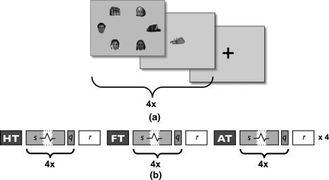
a: The layout of a task block in the free viewing experiment: A block consists of four stimuli, whose durations are determined pseudorandomly between 8 and 18 s, composed of house and face objects, each followed by a quiz item (3 s). A block starts with an instruction (10 s), indicating the task condition, and ends with a fixation cross (10 s). b: Schematic representation of the free viewing experiment. HT, FT, and AT denote the presentation of the instruction screens for House Task, Face Task, and All Task, respectively; s represents stimulus presentation (with varying duration); q represents the presentation of the quiz item; r represents a resting period with the presentation of a fixation cross.

Three different tasks could be given to the observer: “Look at faces” (Face Task, FT), “Look at houses” (House Task, HT), or “Free viewing” (All Task, AT). A task block started with an instruction screen (10 s), followed by four repetitions of stimulus screens (each with different stimuli and varying presentation time) and a quiz screen. A task block ended with a fixation cross (10 s) (Fig. 1b). Due to the varying duration of the presentation time of individual stimuli, the blocks also varied in their total duration. During the house task, subjects were quizzed only on house items. During the face task, only face items were tested. In the all task, subjects could be asked about the presence of both types of objects.

In total, we recorded eye movements for 32 stimuli per task condition per subject (2 (free viewing experiments) × 4 (stimuli per task block) × 4 (iterations of a task block)). Although observers could be instructed to look at specific items, the order in which they chose to do so was left entirely to the subject (and they could make errors). Hence, viewing behavior in all tasks was unrestricted.

Eye‐Tracking Analysis

Fixations were calculated based on the recorded gaze behavior using IViewX software (SMI, Teltow, Germany). A fixation duration threshold of 80 ms was used. Fixations having the same position and separated by a short blink were concatenated. Subsequently, using in‐house developed software, each fixation was labeled according to the inspected object and the task of the trial. The possible fixation labels are shown in Table I. To label fixations, six circular areas of interest (110 pixel radius) were defined and placed on the location of each object (objects covered ∼150 × 150 pixels each). In the remainder of the analysis, only fixations made during the presentation of a stimulus were taken into account. We excluded fixations falling outside the areas of interest. This removed ∼15% of the fixations made during the stimulus presentations. These were almost entirely fixations directed at the centre of the screen.

Table I.

Summary statistics of fixations used in the fMRI analysis (i.e., made toward an object during the presentation of a stimulus)

Task	Fixated object	Condition	Mean percentage (SD)	Total number of fixations
All	House	H‐AT	18.3 (±3.0)	4,059
House	House	H‐HT	25.4 (5.0)	5,691
Face	House	H‐FT	10.2 (4.0)	2,039
All	Face	F‐AT	16.2 (3.3)	3,496
House	Face	F‐HT	12.7 (5.1)	2,593
Face	Face	F‐FT	17.1 (4.8)	3,854
Total			99.9	21,732

Results are totals for all 20 subjects. Total in column Mean percentage does not sum up to 100% due to rounding errors.

Histograms and density histograms were constructed for all fixations grouped per fixation type. In addition, the same graphs were constructed for target fixations, where dwell times were concatenated for subsequent fixations at the same target type. To further investigate the temporal characteristics of the eye movement data, we created an autocorrelation plot of all eye movements for each task. Sequences of inspected object types were extracted and concatenated per task type. Autocorrelation values were calculated using a lag of 1–500 time points (i.e., 10 s).

FMRI Analysis

All fMRI analyses were performed using SPM5 (Wellcome Trust Centre for Neuroimaging, London, UK) in Matlab (Mathworks, Natick, MA). Preprocessing consisted of realignment to correct for subject movement, coregistration to align all functional data to subject's anatomical volume, normalization to convert all images to Montreal Neurological Institute (MNI) space, and spatial smoothing with a Gaussian kernel of 8 mm (full width at half maximum). No slice timing correction was applied.

Localizer Experiment

After convolution with the informed basis set [Friston et al., 1998a], standard univariate t‐tests were used to calculate differences between house and face conditions (contrast “face > house,” amplitude component only). These contrasts were fed into a second level random‐effect analysis using a one‐way ANOVA. The resulting T‐map of this statistical analysis was used to create regions‐of‐interest masks applied in the analysis of the free viewing experiment.

Free Viewing Experiment

We modeled all six categories of both face fixations (F‐FT, F‐HT, and F‐AT) and house fixations (H‐FT, H‐HT, and H‐AT), using the same analysis as in the localizer experiment. Standard univariate t‐tests were created for each component individually against baseline and resulted in three parameter estimates for each fixation category.

Estimation Efficiency

To assess the estimation efficiency of each design, we calculated the ratio between the biased efficiency and the optimal efficiency term, using the mean corrected design matrix after convolution and high‐pass filtering [Dale, 1999; Liu et al., 2001].

ROI Analysis

Four regions of interest were defined from the T‐maps of the localizer experiment, using MarsBar [Brett et al., 2002]. Left and right Fusiform Face Area (FFA) and bilateral Parahippocampal Place Area (PPA) were drawn using uncorrected P‐values of 0.01 (Fig. 5). The coordinates of all four areas were in accordance with the relevant literature [Grill‐Spector et al., 2004; Kanwisher et al., 1997] (centres in MNI coordinates are as follows: left FFA −40.4 x −50.1 y −19.4 z; right FFA 42.7 x −49 y −17.2 z; left PPA −24.4 x −49.3 y −9.23 z; and right PPA 26.6 x −47.1 y −10.6 z). Furthermore, a spherical region in the early visual cortex of each hemisphere was defined with a radius of 10 mm around the centre locations 28.0 x −71.0 y −16.0 z (right hemisphere) and −34.0 x −71.0 y −16.0 z (left hemisphere) (Supporting Information, Fig. 1).

Figure 5.

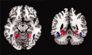
Axial (left) and coronal (right) views of regions of interest. Red indicates Parahippocampal Place Area (PPA) and blue denotes Fusiform Face Area (FFA). [Color figure can be viewed in the online issue, which is available at wileyonlinelibrary.com.]

Differences in the BOLD responses evoked by each fixation class were investigated by modeling their associated haemodynamic responses. At the single subject level, a model was defined using both the onsets and durations of fixations of all fixation categories. These models were estimated in SPM5 (Restricted Maximum Likelihood estimation) using the informed basis set (represented by an amplitude, derivative, and dispersed parameter) [Friston et al., 1998b]. For each individual observer within the six ROIs, we obtained the parameter estimates. Next, these individual parameter estimates were averaged across observers, resulting in three estimates per ROI per fixation category. Consequently, summing the three parameter estimates multiplied with their basis function (from the informed basis set) provided a haemodynamic response.

The procedure described above was repeated using a Fourier basis set with five components filtered with a Hanning window. For both basis sets, we assumed that the event‐related response started and ended at zero signal intensity. Furthermore, two F‐tests were performed for each ROI in SPM5 after applying the small volume correction in SPM with a False Discovery Rate correction of P < 0.05. First, an F‐test was performed to investigate a main effect of the task on haemodynamic responses. The second F‐test was performed to test for differences between house and face fixations. Finally, F‐tests were performed to investigate group differences of combined shape/amplitude response between each possible pairing of conditions for each ROI, small volume corrected at P < 0.001.

Multivariate Analysis

This second experiment entailed multivariate classification based on fixations. We extracted the BOLD voxelwise time course (32 s, 16 data points) following each fixation within the ROIs of unsmoothed fMRI data. These time courses (for each voxel) were concatenated into a single feature vector (hereinafter called “example”) and labeled according to the fixation class. Since fixations were generally shorter than the duration of a single volume, there were usually multiple fixations within the recording of one time point (i.e., volume). To overcome this problem, the labeling for an example was based on the class of the longest fixation during a TR. Next, we used support vector machines (LibSVM, [Chang and Lin, 2001]) within a Matlab environment (version 7.4) to calculate a high‐dimensional plane that separates the fixations based on the feature differences between the classes. A linear kernel was used, since we had relatively few examples and a large number of dimensions [Mourao‐Miranda et al., 2005].

Three classification analyses were performed. The first used labels of each fixation category, including task and inspected object. To investigate task and object inspected component separately, we performed similar classification analyses, where labeling was based only on either component.

For each classification analysis, we obtained a minimum of 10 and maximum of 25 examples for each condition. To determine the significance of the resulting classification performance, we compared it with classification performance from random permutations. Permutation testing was done by randomly permuting the class labels of the examples and measuring the classifier performance across 1,000 iterations to obtain chance levels and confidence intervals [Nichols and Holmes, 2001]. Significance levels of the true classification scores were determined by investigating the distribution of the permutation test, resulting in a P‐value for each classification score (Table II). All classifications were run within observer. To assure independence, training and test sets were obtained from separate free viewing experiments.

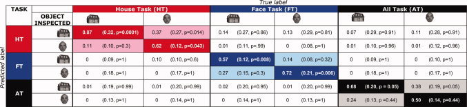
Table II.

Classification scores for longest fixations during a TR [Color table can be viewed in the online issue, which is available at wileyonlinelibrary.com.]

Correct scores are displayed on the diagonal. Chance levels are based on 1000 permutations (displayed between brackets). P‐values represent the fraction of permuted classifications that score higher than the correctly labeled dataset.

RESULTS

Fixation Distributions

Figure 2a shows the distributions of all fixation durations in each category. Compared with those made during instructed viewing (HT and FT), fixation durations for the “all” task (AT) were slightly shorter (confirmed by a two‐sample t‐test, P‐value: 2.2e⁻¹⁶). Figure 2b shows dwell times per fixation category. To calculate dwell time, consecutive fixations on the same type of object were concatenated. In addition, Figure 3 shows distributions of interfixation intervals per fixation category. Interfixation intervals were defined as the difference between onsets of two subsequent fixations within the same category. Figure 4 shows the autocorrelation of the eye movement signal, indicating that autocorrelation values of all three tasks are highly similar and nonzero.

Figure 2.

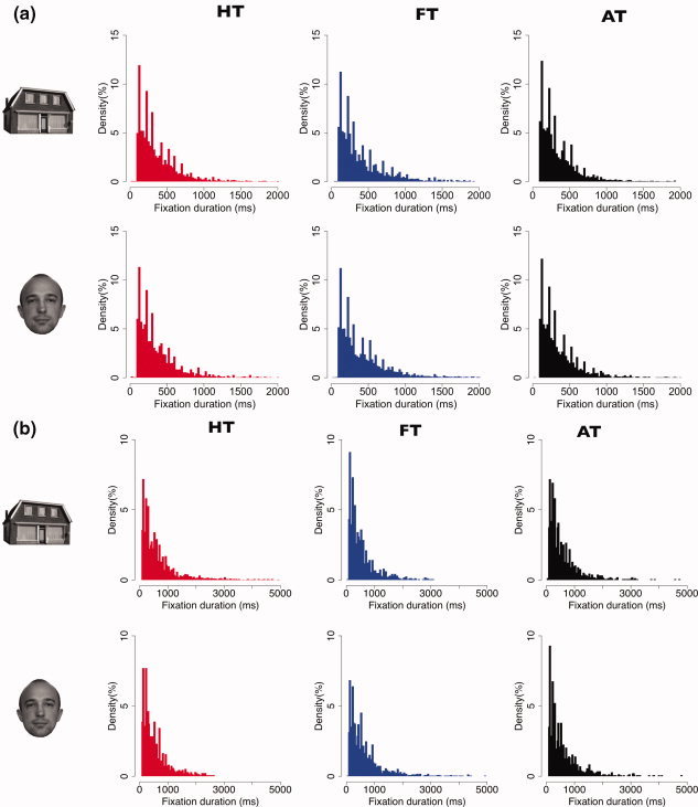
a: Density histograms indicating fixation durations per fixation category used in the fMRI analysis (bin size = 25 ms). HT, FT, and AT denote House Task, Face Task, and All Task, respectively. b: Density histograms indicating dwell times per fixation category used in the fMRI analysis (bin size = 25 ms). HT, FT, and AT denote House Task, Face Task, and All Task, respectively. [Color figure can be viewed in the online issue, which is available at wileyonlinelibrary.com.]

Figure 3.

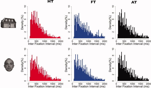
Density histograms indicating interfixation intervals per fixation category used in the fMRI analysis (bin size = 25 ms). HT, FT, and AT denote House Task, Face Task, and All Task, respectively. [Color figure can be viewed in the online issue, which is available at wileyonlinelibrary.com.]

Figure 4.

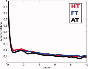
Autocorrelation plot of object inspected per task for lags up to 10 s. HT, FT, and AT denote House Task, Face Task, and All Task, respectively. [Color figure can be viewed in the online issue, which is available at wileyonlinelibrary.com.]

Localizer Experiment

Figure 5 shows the locations of the left and right PPA and FFA, as found on the group‐normalized brain using the localizer experiment. Together with the two control regions in the early visual cortex (Supporting Information), these areas were subsequently used as regions‐of‐interest to investigate fixation‐related brain activity.

Fixation‐Related Brain Activity

To make sure that the subjects performed the required tasks, we examined their scores on the Sternberg memory task. Average performance was 75% (±11% SD) correct for both the HT and FT and 40% (±11% SD) for the AT, which is not surprising given that the AT requires remembering double the number of items. We conclude that subjects performed the tasks appropriately. These scores were not used in the further fMRI analyses.

To investigate the pattern of activity within the three pairs of ROIs, we modeled the haemodynamic responses associated with each type of fixation. Figure 6 depicts average modeled responses for left and right FFA, PPA and the early visual cortex, and split according to ROI, task, and object inspected using the informed basis set (Fig. 3 in the Supporting Information shows results for the models estimated using the Fourier basis set with a Hanning window).

Figure 6.

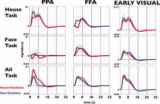
Modeled haemodynamic responses following house fixations (red) and face fixations (blue) in three task conditions for FFA, PPA, and early visual regions of interest (averaged across left and right hemispheres). Modeling is based on the informed basis set with three components (HRF, derivative, and the dispersed of the HRF). Dashed lines indicate standard error of the mean. [Color figure can be viewed in the online issue, which is available at wileyonlinelibrary.com.]

Figure 6 shows that BOLD activations differ most notably for the different ROIs. In particular in the PPA, but also in early visual cortex, the type of task shows a marked effect. Again in the PPA, relatively marked differences in modeled BOLD response can be noted for the two types of fixations (house or face fixation). These observations were confirmed by statistical tests that were performed independently for the ROIs in each hemisphere. An F‐test revealed a main effect of task in both left and right PPA (F(3,357) values: 84.5 (P < 0.001) and 136.8 (P‐value < 0.001), respectively) and left and right visual areas (F(3,357) values: 182.6 (P‐value < 0.001) and 191.9 (P‐value < 0.001), respectively), but not in the FFA. A main effect of fixation type was found in both left and right PPA (F(3,342) values: 44.0 and 69.9, respectively (P‐value < 0.001). No significant effect of fixation type was found in either FFA or the early visual regions. The estimation efficiency—averaged across subjects—was 0.16 (range 0.11–0.25).

Classification of Fixation Types

Using fixations as events, we found BOLD responses that differed to various extents depending on ROI, task, and type of fixated object. Hence, this suggests it may be possible to “read” the BOLD response following an individual fixation. Using SVMs, we therefore classified the BOLD responses following longest fixations, in order to determine the associated task and object inspected. Furthermore, in two separate experiments, we investigated the possibility of classifying based on task only and object inspected only. Table II shows the classification based on the combination of task and object inspected. These scores indicate that we can use the BOLD responses associated with fixations to classify with above chance performance task, and in some cases the inspected object. To make it easier to read the table, we have provided an example. Of all actual fixations made toward a house object during the house task (i.e., the first column from Table II), 87% were correctly classified (i.e., as a house fixation made during the house task). When we randomly permuted the labels for this same dataset, the score was 32%, thus indicating chance level performance. The P‐value (shown in brackets in each table cell) indicates the fraction of permuted classifications that scored higher than the correctly labeled dataset. In the house task, 11% of the house fixations were classified as face fixations; so, in these cases, only the task was correctly classified. Note that even in the All task (AT), we could still classify above chance that an observer was inspecting a house picture.

Tables III and IV show classifications that were restricted to either task (Table III) or fixation type (Table IV). Task classification showed a better performance compared with inspected object classification.

Table III.

Classification scores for task using longest fixations during a TR

Type	Score (%)	P‐value	Random permutation baseline (%)
House task (HT)	80	0.05	40
Face task (FT)	64.5	0.045	40
All task (AT)	89.5	0.04	26

Chance levels are based on 1,000 permutations (displayed between brackets). P‐values represent the fraction of permuted classifications that score higher than the correctly labeled dataset.

Table IV.

Classification scores for object inspected using longest fixations during a TR

Type	Score (%)	P‐value	Random permutation baseline (%)
House fixations	78.6	0.03	50
Face fixations	61.7	0.025	50

Chance levels are based on 1,000 permutations (displayed between brackets). P‐values represent the fraction of permuted classifications that score higher than the correctly labeled dataset.

DISCUSSION

The main finding of this study is that fixation‐based event‐related (FIBER) analysis of fMRI signals reveals meaningful spatiotemporal patterns of activation. We have shown that FIBER is feasible, despite the nonrandom properties and relatively brief duration of fixation events, and using relatively standard fMRI scan parameters. Therefore, the FIBER approach allows natural viewing behavior to be incorporated in the analysis of future fMRI experiments. A second finding is that this type of analysis can also reveal the context in which a fixation occurred (in our specific experiment, the task situation).

We have demonstrated the feasibility of FIBER in two ways. First, in two brain areas (PPA and early visual areas), we have shown that fMRI signals following fixations have a distinct task‐dependent shape and amplitude. In the PPA regions, the fMRI responses also differed for the type of object inspected. Second, using multivariate analysis to classify the longer duration fixations, we have shown that the BOLD response contains the information necessary to deduce the object inspected for individual fixations as well as their task context. We will now discuss these results and approaches in more detail.

The first question is, why does FIBER actually work? When participants perform a task, for example the house task, they repeatedly fixate houses. Their eyes probably dwell for a while on a particular house (Fig. 2a,b), even fixating different aspects of that stimulus and then move on to another house stimulus. Occasionally, they may glance at a face target. Consequently, participants spend long enough periods of time on distinct target types (median dwell time on type of object) to allow estimation of the brain response associated with task and object inspected. This can be quantified by calculating the “estimation efficiency” for the experiment [Dale, 1999; Liu et al., 2001]. For the first‐level models, the average estimation efficiency was 0.16, with a range (0.11–0.25). This is comparable to efficiencies for other, self‐paced, event‐related experiments previously performed at our institute (0.05–0.6) [Demenescu et al., 2009; Meppelink et al., 2009]. This quantification of the estimation efficiency thus confirms that FIBER analysis can work.

Fixation‐Related Brain Activity

To assess the feasibility of using FIBER, we first modeled haemodynamic responses for the PPA, FFA, and the early visual areas using the informed basis set (Fig. 6). We found that responses in the PPA and the early visual areas were significantly different for each task. So, even though participants gazed at the same type of objects, responses were different depending on the task. For the PPA, this could indicate that attention to houses (rather than faces) modulates its response [O'Craven et al., 1999]. The fact that this also occurs in the early visual cortex is more surprising and indicates that responses in this region do not simply reflect stimulus content.

Activation patterns in PPA and FFA do not simply reflect responses in the early visual cortex. For example, in the early visual cortex, responses did not differ for fixation category, whereas this was the case in the PPA (most prominent in the All Task). Hence, as the fixation‐related activity propagates from the early visual to higher order regions, specificity in the response increases. This confirms that fixation‐based event‐related responses reveal meaningful activation patterns. In summary, our analysis of fixation‐related brain activity reveals that responses associated with fixations can carry a unique BOLD “fingerprint,” i.e., they can be distinctive.

However, the specificity and distinctiveness of these responses varies per region and may even differ for different tasks within a region. Unlike those in the PPA, responses in the FFA were not significantly modulated by task or fixated object. This was somewhat unexpected. An explanation could be that the FFA location shows more variation between participants. The FFA mask was based on a second level analysis. It may therefore not capture the most sensitive region in each participant. Another explanation could be that the FFA is also responsive to face stimuli in the peripheral visual field. The stimuli in our study always contained faces. If the presence of a face in peripheral view were sufficient to activate the FFA to near its maximum level, this would reduce the attainable modulation.

We previously referred to the finding that each condition has a distinct response (this is shown in Fig. 6). Neither the autocorrelation plots nor the histograms of fixation durations and interfixation intervals showed a marked difference in temporal behavior for the fixations under these different conditions. Hence, the differences in the BOLD responses following fixations are not related to the eye movement dynamics. To assess whether the differences in response are a consequence of the HRF model used, responses were also modeled using a Fourier basis set (Fig. 3 in the Supporting Information). This confirmed the differences in the response of the PPA (Tables I and II in the Supporting Information) for the task conditions. In the PPA, responses following fixations on different objects within a task were also significantly different2. Hence, we conclude that the differences in the BOLD responses following fixations are not only related to the task but also to the object inspected.

There are a number of ways in which task‐related differences could affect fixation‐related responses. Extraction of information from the retinal image is only one aspect of the processing taking place during and following a fixation. For example, subsequent saccade planning also influences cortical activity and may influence the fixation‐associated response in a task‐dependent manner. For example in the house task, one expects subjects to use their peripheral vision to localize potential house targets. In the all task condition, this aspect is irrelevant and the participant can simply saccade to any object. In addition, the memory component of the delayed‐match‐to‐sample test, which obviously exceeds the duration of a fixation, could affect the BOLD response in a task‐dependent manner.

On the basis of earlier reports on the optimality of event timings for maximal detection and estimation in fMRI [Birn et al., 2002], we inferred that fixations would be suboptimal for rapid event‐related designs. Despite these suboptimal characteristics, we ascertained clear fixation‐related activations. In general, we found that the peak of the activation occurred at around 4 s postevent. While this is shorter than the more generally assumed peak at 5 to 6 s postevent, it closely matches earlier reports on reduced peak latencies in case of brief events in rapid event‐related designs [Hinrichs et al., 2000; Kim et al., 1997; Liu etal., 2000].

Classification of Fixations

Using multivariate pattern analysis (MVPA), we have shown that the nature of longer fixations can be decoded from the brain response. On the basis of the BOLD response following longer fixations, we could fairly successfully decode the object that observers gazed at during an individual fixation as well as the task context in which this occurred. Table IV shows that classification of both task and object inspected was successful (i.e., scores on the diagonal are well above chance). This behavior was expected, given the differences in results for the average modeled HRF (i.e., each fixation class was associated with a distinct HRF pattern). Still, this additional result is important, as the SVMs only have the data and not the modeled responses available for training and classification. Moreover, the successful decoding efforts support our idea that a fixation can be seen as a unit of information.

Hence, our work suggests that FIBER analysis of fMRI data is viable and is able to provide information about cortical processing in different contexts and with configurations of stimuli. At present, and with the standard scanning parameters used here, FIBER still has some limitations. We envision a number of options to improve on the present approach. First, FIBER analysis will presumably improve when applied in combination with an fMRI acquisition using higher temporal resolutions [Sabatinelli et al., 2009]. Second, for the current task and stimuli, FIBER appears to work better in some regions (PPA) than others (FFA, early visual cortex). Therefore, studies intending to apply the method may choose to first use FIBER in a localizer experiment to select regions‐of‐interest that distinguish between the given tasks or stimuli. The use of more specific localizers and individually determined ROIs may also help improve the sensitivity for differentiating fixation‐related responses. Likewise, in this study, we chose functionally defined regions over anatomically defined regions, expecting higher sensitivity.

CONCLUSIONS

We have shown that event‐related fMRI analysis based on fixations is viable, despite the less favorable temporal and statistical characteristics of fixations. The present experiment used standard scanning parameters, which resulted in temporal undersampling. Nevertheless, the average haemodynamic responses revealed distinct fixation‐related cortical activation patterns for each task. Furthermore, within specific regions, we could even significantly differentiate the responses for different objects inspected. Using multivariate pattern recognition, we have also shown that, at the level of individual fixations, cortical activation patterns can be used to classify the object inspected and the task context. Thus, by using FIBER analyses, paradigms can be envisaged that allow unrestrained, natural viewing behavior in fMRI research.

Supporting information

Additional Supporting Information may be found in the online version of this article.

Supporting Information

REFERENCES

- Birn RM, Saad ZS, Bandettini PA ( 2001): Spatial heterogeneity of the nonlinear dynamics in the FMRI BOLD response. Neuroimage 14: 817–826. [DOI] [PubMed] [Google Scholar]
- Birn RM, Cox RW, Bandettini PA ( 2002): Detection versus estimation in event‐related fMRI: Choosing the optimal stimulus timing. Neuroimage 15: 262–264. [DOI] [PubMed] [Google Scholar]
- Boynton GM, Engel SA, Glover GH, Heeger DJ ( 1996): Linear systems analysis of functional magnetic resonance imaging in human V1. J Neurosci 16: 4207–4221. [DOI] [PMC free article] [PubMed] [Google Scholar]
- Brainard DA ( 1997): The psychophysics toolbox. Spat Vis 10: 433–436. [PubMed] [Google Scholar]
- Brett M, Anton JL, Valabregue R, Poline JB ( 2002): Region of interest analysis using an SPM toolbox. In: 8th International Conference on Functional Mapping of the Human Brain, Vol. 16.
- Buckner RL ( 1998): Event‐related fMRI and the hemodynamic response. Hum Brain Mapp 6: 373–377. [DOI] [PMC free article] [PubMed] [Google Scholar]
- Burock MA, Buckner RL, Woldorff MG, Rosen BR, Dale AM ( 1998): Randomized event‐related experimental designs allow for extremely rapid presentation rates using functional MRI. Neuroreport 9: 3735–3739. [DOI] [PubMed] [Google Scholar]
- Chang H‐C, Lin CJ ( 2001): LIBSVM: A library for support vector machines.
- Cornelissen FW, Peters EM, Palmer J ( 2002): The eyelink toolbox: Eye tracking with MATLAB and the psychophysics toolbox. Behav Res Methods Instrum Comput 34: 613–617. [DOI] [PubMed] [Google Scholar]
- Dale AM ( 1999): Optimal experimental design for event‐related fMRI. Hum Brain Mapp 8: 109–114. [DOI] [PMC free article] [PubMed] [Google Scholar]
- Dale AM, Buckner RL ( 1997): Selective averaging of rapidly presented individual trials using fMRI. Hum Brain Mapp 5: 329–340. [DOI] [PubMed] [Google Scholar]
- Dalton KM, Nacewicz BM, Johnstone T, Schaefer HS, Gernsbacher MA, Goldsmith HH, Alexander AL, Davidson RJ ( 2005): Gaze fixation and the neural circuitry of face processing in autism. Nat Neurosci 8: 519–526. [DOI] [PMC free article] [PubMed] [Google Scholar]
- Demenescu LR, Kortekaas R, Renken R, van Tol MJ, van der Wee NJA, Veltman DJ, den Boer JA, Aleman A ( 2009): The Netherlands study of anxiety and depression: Amygdala response to facial expressions. Neuroimage 47: S183. [Google Scholar]
- Epstein R, Kanwisher N ( 1998): A cortical representation of the local visual environment. Nature 392: 598–601. [DOI] [PubMed] [Google Scholar]
- Friston KJ, Josephs O, Rees G, Turner R ( 1998a): Nonlinear event‐related responses in fMRI. Magn Reson Med 39: 41–52. [DOI] [PubMed] [Google Scholar]
- Friston KJ, Fletcher P, Josephs O, Holmes A, Rugg MD, Turner R ( 1998b): Event‐related fMRI: Characterizing differential responses. Neuroimage 7: 30–40. [DOI] [PubMed] [Google Scholar]
- Glover GH ( 1999): Deconvolution of impulse response in event‐related BOLD fMRI. Neuroimage 9: 416–429. [DOI] [PubMed] [Google Scholar]
- Grill‐Spector K, Knouf N, Kanwisher N ( 2004): The fusiform face area subserves face perception, not generic within‐category identification. Nat Neurosci 7: 555–562. [DOI] [PubMed] [Google Scholar]
- Haynes J‐D, Rees G ( 2006): Decoding mental states from brain activity in humans. Nat Rev Neurosci 7: 523–534. [DOI] [PubMed] [Google Scholar]
- Hinrichs H, Scholz M, Tempelmann C, Woldorff MG, Dale AM, Heinze HJ ( 2000): Deconvolution of event‐related fMRI responses in fast‐rate experimental designs: Tracking amplitude variations. J Cogn Neurosci 12 ( Suppl 2): 76–89. [DOI] [PubMed] [Google Scholar]
- Josephs O, Turner R, Friston K ( 1997): Event‐related fMRI. Hum Brain Mapp 5: 243–248. [DOI] [PubMed] [Google Scholar]
- Kanwisher N, McDermott J, Chun MM ( 1997): The fusiform face area: A module in human extrastriate cortex specialized for face perception. J Neurosci 17: 4302–4311. [DOI] [PMC free article] [PubMed] [Google Scholar]
- Kim S‐G, Richter W, Ugurbil K ( 1997): Limitations of temporal resolution in functional MRI. Magn Reson Med 37: 631–636. [DOI] [PubMed] [Google Scholar]
- Kriegeskorte N, Bandettini P ( 2007): Analyzing for information, not activation, to exploit high‐resolution fMRI. Neuroimage 38: 649–662. [DOI] [PMC free article] [PubMed] [Google Scholar]
- Liu H‐L, Pu Y, Nickerson LD, Liu Y, Fox PT, Goa J‐H ( 2000): Comparison of the temporal response in perfusion and BOLD‐based event‐related functional MRI. Magn Reson Med 43: 768–772. [DOI] [PubMed] [Google Scholar]
- Liu TT, Tong F, Buxton RB ( 2001): Detection power, estimation efficiency and predictability in event‐related fMRI. Neuroimage 13: 759–773. [DOI] [PubMed] [Google Scholar]
- Martinez‐Conde S, Macknik SL, Hubel DH ( 2004): The role of fixational eye movements in visual perception. Nat Rev Neurosci 5: 229–240. [DOI] [PubMed] [Google Scholar]
- Meppelink AM, de Jong BM, Renken R, Leenders KL, Cornelissen FW, van Laar T ( 2009): Impaired visual processing preceding image recognition in Parkinson's disease patients with visual hallucinations. Brain 132: 2980–2993. [DOI] [PubMed] [Google Scholar]
- Mourao‐Miranda J, Bokde ALW, Born C, Hampel H, Stetter M ( 2005): Classifying brain states and determining the discriminating activation patterns: Support vector machine on functional MRI data. Neuroimage 28: 980–995. [DOI] [PubMed] [Google Scholar]
- Nichols TE, Holmes AP ( 2001): Nonparametric permutation tests for functional neuroimaging: A primer with examples. Hum Brain Mapp 15: 1–25. [DOI] [PMC free article] [PubMed] [Google Scholar]
- O'Craven KM, Downing P, Kanwisher N ( 1999): fMRI evidence for objects as the units of attentional selection. Nature 401: 584–587. [DOI] [PubMed] [Google Scholar]
- Rosen BR, Buckner RL, Dale AM ( 1998): Event‐related functional MRI: Past, present, and future. Proc Natl Acad Sci USA 95: 773–780. [DOI] [PMC free article] [PubMed] [Google Scholar]
- Saad ZS, Ropella KM, DeYoe EA, Bandettini PA ( 2003): The spatial extent of the BOLD response. Neuroimage 19: 132–144. [DOI] [PubMed] [Google Scholar]
- Sabatinelli D, Lang PJ, Bradley MM, Costa VD, Keil A ( 2009): The timing of emotional discrimination in human amygdala and ventral visual cortex. J Neurosci 29: 14864–14868. [DOI] [PMC free article] [PubMed] [Google Scholar]
- Yarbus A ( 1967): Eye Movements and Vision. New York: Plenum Press. [Google Scholar]
Associated Data
This section collects any data citations, data availability statements, or supplementary materials included in this article.
Supplementary Materials