Variability of fMRI‐response patterns at different spatial observation scales

Abstract

Functional organization units of the cerebral cortex exist over a wide range of spatial scales, from local circuits to entire cortical areas. In the last decades, scale‐space representations of neuroimaging data suited to probe the multi‐scale nature of cortical functional organization have been introduced and methodologically elaborated. For this purpose, responses are statistically detected over a range of spatial scales using a family of Gaussian filters, with small filters being related to fine and large filters—to coarse spatial scales. The goal of the present study was to investigate the degree of variability of fMRI‐response patterns over a broad range of observation scales. To this aim, the same fMRI data set obtained from 18 subjects during a visuomotor task was analyzed with a range of filters from 4‐ to 16‐mm full width at half‐maximum (FWHM). We found substantial observation‐scale‐related variability. For example, using filter widths of 6‐ to 8‐mm FWHM, in the group‐level results, significant responses in the right secondary visual but not in the primary visual cortex were detected. However, when larger filters were used, the responses in the right primary visual cortex reached significance. Often, responses in probabilistically defined areas were significant when both small and large filters, but not intermediate filter widths were applied. This suggests that brain responses can be organized in local clusters of multiple distinct activation foci. Our findings illustrate the potential of multi‐scale fMRI analysis to reveal novel features in the spatial organization of human brain responses. Hum Brain Mapp, 2011. © 2011 Wiley‐Liss, Inc.

INTRODUCTION

Spatial patterns in images exist over a broad range of scales. To account for this property, images can be embedded into a family of derived images—the so‐called scale‐space representation—with spatial resolution as a parameter [Iijima, 1962; Koenderink, 1984; Witkin, 1983]. In image processing and computer vision research, the best‐studied scale‐space representation is the Gaussian scale‐space model derived through convolution of the original image with a family of Gaussian filters [Florack et al., 1992; Koenderink, 1984; Kuijper and Florack, 2003; Lindeberg, 1994]. The width of the Gaussian filter determines scale, with narrow and broad filters being related to scales with fine and coarse resolutions, respectively. Depending on the scale, different spatial patterns of an image may be enhanced. As illustrated in Figure 1, this is particularly important for analysis of noisy images, as, according to the matched filter theorem [Rosenfeld and Kak, 1982], a signal embedded in (white) noise is optimally detectable by smoothing with a filter whose size and shape match those of the signal. Scale selection implies a suitable selection of observation scales so that the relevant patterns in an image are represented [Lindeberg, 1999]. Appropriate scale selection is therefore crucial for obtaining meaningful and comprehensive image representations.

Figure 1.

Spatial smoothing effects on a noisy image with structure at different spatial scales. Three image components—(a) white noise (b) five Gaussian‐shaped signals of a small size (6‐pixel standard deviation), and (c) three Gaussian shaped signals with larger size (24‐pixel standard deviation)—were added to generate the original image in (d). This image was then smoothed with a broad and a narrow 2D Gaussian smoothing filter, with the filter widths matching the large (c) and small (b) signal, respectively, to generate the two smoothed versions of the image (e) and (f). All images are scaled to their individual maximum (corresponding to the yellow color). In line with the matched filter theorem [Rosenfeld and Kak, 1982] stating that a signal in white noise is optimally detected by smoothing with a filter whose size and shape match those of the signal, the large signal is well recovered using the matching, broad filter, corresponding to a coarse observation scale, and the small signal using the matching, narrow filter, corresponding to a finer observation scale. As illustrated, very different spatial structures may be revealed from the same image if it is represented at different spatial scales. [Color figure can be viewed in the online issue, which is available at wileyonlinelibrary.com.]

Functional images of the human brain obtained from positron emission tomography (PET) or functional magnetic resonance imaging (fMRI) that are broadly used to investigate human brain function also have the scale dimension. This topic in functional brain imaging was originally addressed in the work by [Poline and Mazoyer, 1994a, b]. However, scale‐space searches in PET or fMRI research are facing additional challenges, since the aim is not just to represent functional data on multiple spatial scales, as is often the objective in computer vision and image processing, but also to detect brain responses in a noisy background using statistical methods at multiple spatial scales. To this end, Gaussian smoothing with filters of different sizes are typically applied to functional datasets before statistical inference. However, due to the non‐linearity involved, statistical results derived from functional data at a coarser scale are not a smoothed version of the results obtained at finer scales. Therefore, statistical inference must be repeated for each version of functional data obtained by spatial filtering with filters of different sizes. These additional statistical tests resulting from search over scales must be accounted for in the control for false positive error rates under multiple test conditions. For this purpose, a number of methods for statistical scale‐space searches in neuroimaging data have been developed and refined over the last decades [Worsley et al., 1996].

Poline and Mazoyer demonstrated a better sensitivity to detect brain activation from PET imaging data using a multi‐filter approach considering multiple spatial scales as compared to a single‐filter approach [Crivello et al., 1995; Poline and Mazoyer, 1994a, b]. Siegmund and Worsley integrated scale‐space searches with Gaussian random field theory, giving appropriate rejection thresholds when testing for a signal with unknown location and scale using a spherical Gaussian kernel in a stationary Gaussian random field [Siegmund and Worsley, 1995]. A unified P‐value for local maxima in 4D scale‐space searches (three spatial dimensions and one extra dimension for scale) was presented [Worsley et al., 1996] and later extended to higher dimensions and to χ² random fields [Worsley, 2001]. Scale‐space searches were further generalized to rotating filters with a better detection power for ellipsoidally shaped brain responses [Shafie et al., 2003] and to cortical surface‐constrained analysis of fMRI data [Andrade et al., 2001]. When examining each scale separately, multiple clustered peaks may be blurred together and detected as a single wide peak at a larger scale [Worsley et al., 1996]. This issue has been addressed by analyzing the deep structure of scale‐space representations, i.e., of all scales simultaneously [Coulon et al., 1997; Lindeberg et al., 1999; Rosbacke et al., 2001], yielding multi‐scale hierarchical representations. Such representations can make the behavior of objects in the image through the scales explicit by providing a comprehensive tree structure of activated brain regions [Lindeberg et al., 1999]. Such a structure may, for instance, show how a cluster of sharp foci detected at a fine image resolution is merged into one activated area at a coarser resolution [Coulon et al., 2000].

In spite of this theoretical and methodological progress, scale‐space searches are rarely used in current functional brain imaging studies. Typically, functional imaging results are obtained using only one single Gaussian smoothing filter. According to a recent review of current fMRI studies, applied filter widths vary from 2‐ to 12‐mm full width at half‐maximum (FWHM) [Breckel, 2007]. In particular for fMRI data, few studies have investigated the effect of spatial smoothing filter width on statistical response maps. Worsley [2001] investigated data from a single subject over a broad range of scales and detected visual stimulation‐related fMRI responses at all scales. In another single‐subject study, higher Z‐scores for fMRI responses in cortical regions were found for narrow (6‐mm FWHM) as compared to broader (10‐ and 14‐mm FWHM) filters, while the opposite was found for subcortical responses [Friston et al., 1996]. Based on the results from a small group of six subjects, another fMRI study came to contrary conclusions, suggesting that narrow filters were more suitable for detecting subcortical and broad filters—for cortical responses [White et al., 2001]. Other studies have emphasized and clearly demonstrated the unwanted over‐smoothing effects on fMRI data in cases where high spatial resolution was important for data interpretation, both on a single‐subject level [Fransson et al., 2002; Geissler et al., 2005] and for group analysis of a sample of eight subjects [Fransson et al., 2002]. Thus, for single‐subject fMRI, only limited data is available on the degree of variability that may be encountered over a range of spatial scales. Moreover, to our knowledge, there is no such data for fMRI group analyses based on a larger sample of subjects.

Against this background, the major aim of the present study was to systematically investigate the degree of variability of fMRI‐response patterns over a broad range of observation scales, based on a larger sample of subjects than in previous studies. To this aim, fMRI data from a visuomotor and an auditory task in a larger sample of subjects than in the previous studies on filter size effects (18 subjects, see above) were analyzed. The approach of the present study was adopted from a recent study investigating scale‐space variability in voxel‐based morphometry (VBM) analyses of diffusion tensor MRI data [Jones et al., 2005]. In this latter study, 3‐D Gaussian filter width was varied from 0 to 16 mm, yielding results that supported completely different interpretations of the VBM data (the importance of the scale space problem for VBM analysis has been repeatedly emphasized also by [Ridgway et al., 2008; Van Hecke et al., 2009]). Taking a similar approach as in the study by Jones et al., we investigated the effect of observation scale on fMRI results, on both individual and group levels.

In contrast to previous studies on the effects of filter width on fMRI analyses, we based the assignment of response peaks to cortical anatomy on a probabilistic atlas system [Amunts et al., 1999, 2003; Choi et al., 2006; Eickhoff et al., 2005; Geyer et al., 1996; Schenker et al., 2008]. Probabilistic anatomical assignment of response peaks to cortical and subcortical structures is increasingly used in current fMRI studies, as it has the advantage of providing information about location and inter‐individual variability of brain areas in a standard reference space. This approach allows for assigning activation sites to histologically defined brain regions in a probabilistic fashion, even if these brain regions are not discernible in structural brain images. To quantify scale effects, we traced the t‐values of response peaks in probabilistically defined anatomical brain regions over a broad range of scales [Andrade et al., 2001]. Our findings demonstrate an observation‐scale‐related variability of response peak assignment to probabilistically defined cortical areas with a substantial impact on the functional interpretation. Thus, our study emphasizes the importance of multi‐scale method application for future fMRI research.

MATERIALS AND METHODS

Subjects

Eighteen healthy subjects participated in the experiment. None of the participants had a history of psychiatric or neurological diseases. According to the Edinburgh handedness questionnaire [Oldfield, 1971], all subjects were right‐handed (mean = 84.95%, range = 75–100%). The study was approved by the Ethics Committee of the University of Freiburg, Germany. Before participation, the subjects signed a written informed consent and they received a modest monetary compensation for participation.

Experimental Set‐Up and Procedure

During the fMRI experiment, 40 short pieces of piano music, each of a 24‐s duration, were presented to the subjects in a random order, using in‐house‐developed presentation software, via magnetic resonance compatible headphones (NordicNeuroLab, Bergen, Norway). After the presentation, the subjects rated each piece on a bipolar assessment scale along the dimensions of valence (ranging from −3 = very unpleasant to 3 = very pleasant) and arousal (ranging from −3 = very calming to 3 = very arousing) using an MRI‐compatible computer mouse, which allowed the subjects to move a white box to the left or the right along the visually presented scale by pressing the corresponding mouse buttons with the right hand. The selected level was marked by the white box, and the remaining six levels were indicated by black boxes. For each of both valence and arousal ratings, a time window of 6 s was available. The position of the white box at the end of the 6‐s period was taken as the subjects' final rating. All subjects were familiarized with this procedure before the fMRI experiment.

In the present study, we analyzed, separately, the responses in the visuomotor system related to the rating task and the responses in the auditory system related to the music stimuli. Further details and the results related to music processing can be found in [Ball et al., 2007; Mutschler, 2007]. These particular tasks were selected since validated a priori assumptions about the involved brain areas exist: for example, for visual stimulation, activation in the visual cortex can be expected, hand movement can be expected to activate the sensorimotor cortex and the processing of music can be expected to activate the auditory cortex. The expected activation areas cover the major portions of the cerebral cortex, i.e., the occipital, parietal, temporal, and frontal lobe, both on the medial wall and on the lateral convexity. This wide‐spread activation pattern was useful for the present study to assure that the found results are not specific to just one region of the human cerebral cortex.

Data Acquisition

Image acquisition started with a localizer scan and a reference scan for distortion correction followed by acquisition of the anatomical T1 whole‐brain data set (7‐min duration): subsequently, the fMRI experiment was conducted as described above with a total scanning time of 43 min.

Functional and structural images were acquired on a 3‐Tesla scanner (Siemens Magnetom Trio, Erlangen, Germany): structural T1‐weighted images were obtained using a MPRAGE sequence (resolution: 1 mm isotropic, matrix: 256 × 256 × 160, TR: 2,200 ms, TI: 1,000 ms, 12° flip angle). The functional images were obtained using a multi‐slice gradient echo planar imaging method (EPI). Each volume consisted of 44 sagittal slices (3‐mm isotropic resolution, matrix: 64 × 64, FOV 192 mm × 192 mm, TR 3,000 ms, TE 30 ms, 90° flip angle). The sagittal slice orientation resulted in significantly lower acoustic noise generated by the imaging gradients. In addition, this orientation in combination with the slice thickness of 3‐mm reduced signal loss in the amygdala region, thus allowing for a more reliable detection of activation [see also Ball et al., 2007]. An accurate registration of the functional and structural images was achieved by online correction of the EPI data for geometric distortions [Zaitsev et al., 2004]. The distortion field was derived from the local point spread function (PSF) in each voxel as determined in a 1‐min reference scan. Prior to distortion correction, the data were motion‐corrected by image realignment with the reference scan using a retrospective 3D algorithm based on the methods as described in [Thesen et al., 2000].

Pre‐Processing and Statistical fMRI Analysis

As mentioned above, motion and distortion correction were performed online during the reconstruction process. All functional images were normalized into the standard space of the Montreal Neurological Institute (MNI) template. Subsequently, 13 differently smoothed functional datasets were generated using 13 3D Gaussian kernels of different sizes, with kernel FWHM equally spaced in 1‐mm steps from 4 to 16 mm. Similar to the study by Jones et al. [2005], linear sampling along the scale dimension was used, because we were interested in the amount of variability that occurs at all scales in the range typically used in current fMRI studies [Jones et al., 2005, also see Introduction and Discussion sections].

For subsequent statistical analysis of the functional data, the timing information of the piano melodies and that of the evaluation periods for valence and arousal after each melody presentation were modeled with a box‐car function convolved with a canonical hemodynamic response function, resulting in three regressors, one—for the piano melodies and two—for valence and arousal ratings, respectively. A high‐pass filter with a cut‐off of 1/128 Hz was applied before parameter estimation. We performed preprocessing and data analysis using SPM5 (Wellcome Department of Cognitive Neurology, London, UK).

On the single‐subject level, fMRI responses related to the visuomotor task of the evaluation periods were calculated for all subjects using a one‐sample t test. Group‐level random effect statistics using a one‐sample t test were then computed to reveal significant responses over the total of 18 subjects. To assure that our results on observation‐scale‐related variability were valid across a wide range of levels of significance, we computed statistical parametric maps at three significance levels: P < 0.05, FWE‐corrected; P < 0.0001 and P < 0.05, both uncorrected. The results at this latter threshold were included to test whether findings of scales without significant responses were possibly due to just‐below‐threshold responses at the more conservative thresholds of P < 0.05 (FWE‐corrected) and P < 0.0001 (uncorrected).

For anatomical assignment, we used probabilistic anatomical maps [Toga et al., 2006]. Due to the visuomotor nature of the task, we determined the following anatomical regions of interest (ROIs) using the maximum probability map (MPM) algorithm proposed by [Eickhoff et al., 2005]: Areas 17 and 18 of the visual cortex, Areas 4a and 4p of the primary motor cortex, Area 6, i.e., the premotor cortex, Areas 1, 2, 3a, and 3b of the primary somatosensory cortex, and Areas 44 and 45 constituting Broca's area. The premotor ROI was further subdivided into the supplementary motor area (SMA), the dorsal, and the ventral premotor cortex (PMd and PMv). Because there are as of yet no probabilistic maps for these subregions of BA 6 available, we defined the SMA as the part of Area 6 where the MNI x‐coordinate was <10 mm, as the SMA in humans has been described as extending onto the lateral cerebral convexity as far as ∼10 mm [Marsden et al., 1996]. The remaining lateral part of Area 6 was subdivided by a plane at z = 50 mm, i.e., PMv was accordingly defined by z = 50 mm and PMd by z > 50 mm. The results of our study, however, did not critically depend on the exact position of this anatomical boundary, and very similar results were obtained when it was shifted within a range of ±5 mm. As anatomical ROIs for the auditory task, we defined the bilateral auditory cortex and BA44 and BA45.

As a next step of analysis, we traced the t values of response peaks over scales. To this end, we determined, for each scale, the maximal t value of all significant response peaks in each of the anatomical ROIs (see Supporting Information Fig. 1). This approach is particularly useful for the purposes of the present study because it reflects the information that is often reported in current fMRI studies (i.e., response peaks and their anatomical assignment). Therefore, changes in peak assignment may critically alter the functional interpretation of an fMRI study (see Discussion for examples). In addition, we also determined the number of significant peaks for each ROI and each smoothing step to identify ROIs where multiple sharp foci converged to a single wide peak at larger smoothing levels.

We performed an additional analysis using an alternative criterion to define anatomical ROIs as previously used in the fMRI literature. This analysis aimed to ensure that our results did not only hold for one specific ROI definition, but were, in fact, more general. The alternative ROI definition was based on the core regions of the probabilistically defined brain areas, requiring an anatomical assignment probability in which a voxel had to belong to a given area in at least 90% of the brains underlying the probabilistic anatomical maps. A similar approach was previously used by [Ball et al., 2007]. In addition to the threshold of 90%, we also tested other thresholds of 60, 70, and 80%, yielding very similar results. Thus, only the results for the 90% threshold are reported. For significant peaks in the anatomical core regions, the same analyses as described above for the ROIs defined using the MPM algorithm were carried out.

To test for the generality of our findings, in addition to the analysis of the visuomotor data sets as described above, we performed the same multi‐filter analysis for fMRI responses during the processing of the auditory stimuli presented to the subjects [see Mutschler et al., 2010 for further details].

RESULTS

In the following, the results from the visuomotor datasets are described. Both individual and group results obtained with different filter widths showed, overall, significant responses in the brain regions with known visual and sensorimotor functions. Results from the analysis of auditory‐related fMRI responses (see Supporting Information Fig. 2) are mentioned when they provide additional or different information. Examples of single‐subject data for different smoothing levels are shown in Figures 2, 3, 4. These examples illustrate the effect of different smoothing filter widths on fMRI‐response maps: for instance, multiple small activation foci can be seen in the left (i.e., contralateral to the side of hand movement) sensorimotor cortex including both primary motor and somatosensory cortices at smaller (<8‐mm FWHM) filter widths. At larger filter widths, however, this cluster of peaks gradually merged into a single wide peak (see Fig. 3).

Figure 2.

Dependence of voxelwise t values on filter width. In the center panel, visuomotor fMRI responses in an individual subject (S10) obtained with 7‐mm FWHM spatial smoothing (P < 10⁻⁵ uncorrected) are shown for an axial slice at the level of the primary motor hand area. For selected voxel positions, the t values of the statistical parametric maps are shown as a function of spatial filter width (FWHM) in the surrounding panels. In each panel, the peak of the t‐trace and the corresponding filter widths are indicated in red. Where the selected voxel position was a local maximum of the t‐map, the t‐trace is plotted in green, else, in black. Filter widths resulting in maximal t values at the selected voxel positions ranged from 3 mm (unfiltered data) in the left posterior parietal cortex (PPC) to 10 mm spatial smoothing in the left primary somatosensory cortex. Furthermore, some voxel positions such as in the right premotor cortex (PM) and the left PPC remained a local maximum across a wide range of resolutions. In other cases, local maxima remained stationary at a given voxel position only over a few filter levels, see the example from the left M1. [Color figure can be viewed in the online issue, which is available at wileyonlinelibrary.com.]

Figure 3.

Example of single‐subject visuomotor‐task‐related fMRI responses. Responses obtained in an individual subject (S10) with spatial smoothing filters ranging from 4‐ to 16‐mm FWHM, P < 10⁻⁵. Results on the top left are from analysis of the unsmoothed functional data at the original 3‐mm isotropic resolution. All results are shown for the same axial slice at the level of the primary motor hand area. Multiple small responses in the left (i.e., contralateral to the side of hand movement) sensorimotor cortex, including the primary motor and the somatosensory cortex, can be seen when using smaller (<8‐mm FWHM) filter widths, as exemplarily marked by a blue circle for the results obtained with 5‐mm FWHM filtering (top center). When applying larger filter widths, this cluster of peaks gradually merged and became a single wide peak. Additional responses at this axial level were found bilaterally in the region of the intrapariatal sulcus (green circles), the supplementary motor area (SMA, black circle), and the right dorsal premotor cortex (magenta circle). [Color figure can be viewed in the online issue, which is available at wileyonlinelibrary.com.]

Figure 4.

Single‐subject result examples. (a) Effects of filter width on response peak t‐values in regions of interest in visual and sensorimotor cortex, results for the left hemisphere of subject S7 (P < 0.0001). T‐values are color‐coded. If no significant peaks were detected for a given ROI and filter width, the corresponding bin is shown in gray. Compare Supporting Information Figure 1 for the procedure used to determine t‐values for ROIs/scales. (b) Number of significant peaks (“N.o.P.”) for each ROI and filter width. We determined the number of significant peaks for each ROI and each smoothing step to identify ROIs where multiple sharp foci found with small filters converged to a single wide peak at larger smoothing levels. The corresponding results for the right hemisphere of S7 are shown in (c) and (d), for S3 in (e)–(h). In different ROIs, the maximal t‐value was observed at different filter widths, for instance, at 4‐mm smoothing for the left BA 18 in S7, at 8 mm for the left BA 4a in S7, and at 12 mm for the right BA 18 in S7. In the latter case, significant responses were found for narrow filters up to 7 mm, resulting in multiple response peaks within the anatomical ROI, and again for broad filters of 12 mm and above, with only a single peak in the area, but not for intermediate filter widths. [Color figure can be viewed in the online issue, which is available at wileyonlinelibrary.com.]

To further characterize the effect of the different filter widths, we traced t values and the number of significant response peaks in anatomical ROIs of the visuomotor cortical network over scales (c.f. also Supporting Information Fig. 1). Results for ROIs both in the right and left hemispheres of subject S7 are shown in Figures 4a–d and for subject S3—in Figures 4e–h. As these examples show, the maximal t values for different anatomical ROIs were observed at different filter widths. For example, in S7, the maximal t value in BA 18 was found at a 4‐mm filter width, at 8‐mm filter width—in the left BA 4a, and at 12‐mm filter width—in the right BA 18. In the latter case, significant responses were found at narrow filter widths up to 7 mm, resulting in multiple response peaks within the anatomical ROI, and, again, at broad filter widths of 12 mm and above—with only a single peak in the ROI but not at intermediate filter widths.

These different behaviors of the t values in anatomical ROIs over scales on a single‐subject level are summarized for all subjects in Figure 5. We distinguished three groups of responses, based on the shape of the curve of t values as a function of scale. Although different groups could have been defined, these three groups were sufficient and well suited to illustrate the variability of the behavior of t values over scales. The three groups are: (1) t value traces with maximal values in the unsmoothed data or for narrow filters (4‐ and 5‐mm FWHM) shown in Figure 5a for results at a threshold of P < 10⁻⁵ and in Figure 5d, for FWE‐corrected results (P < 0.05); (2) t‐value traces with maximal values at intermediate filter widths (6‐ to 8‐mm FWHM); and (3) t‐traces with significant values both for narrow (defined as before) and broad (9‐mm and above FWHM) filters. Generally, it is assumed that FWE correction requires filtering with at least two times the functional voxel size [Friston et al., 1996], therefore the FWE‐corrected results in (Fig. 5d) have to be interpreted with caution and are only included for completeness. Interestingly, in none of the 18 individual datasets did we observe an instance where, for a given anatomical ROI, significant peaks were only found for broad filters (=9 mm), without any significant peak for narrow filters. Examples from each of the three groups were found in a wide range of cortical areas (Fig. 5, small insets in a–f). In the FWE‐corrected results obtained from analyzing the auditory datasets, however, for the left BA45 and the right BA44, significant responses were only found for filter width =10 mm FWHM (Supporting Information Fig. 3).

Figure 5.

Single‐subject result summary. For each anatomical ROI in each subject, the dependence of response peak t values on scale was determined as illustrated in Supporting Information Figure 1, resulting in a “t‐trace” for each ROI in each subject. These t‐traces were sorted into three groups as described below and a mean and standard error was calculated over all t‐traces. (a) shows the resulting mean t‐trace for the first group of t‐traces showing the maximal t‐values either for the unsmoothed data or for narrow filters (4‐ and 5‐mm FWHM) and no second maximum for broad filters. A total of 156 traces, corresponding to 77.6% of all traces detected at this threshold, fell into this group. The anatomical ROIs where these t‐traces were found are indicated by the pie chart (color legend at the bottom of the figure). In (b) the average trace is shown for all ROIs where t‐values where maximal at intermediate filter widths (6‐ to 8‐mm FWHM, this range is indicated by the light gray box). About 25 (12.4%) of all traces were of this type, which occurred in most of the investigated anatomical ROIs. (c) shows traces which had significant t‐values for narrow filters as in (a) and also for broad filters (9‐mm FWHM and above). This type of traces occurred 20 times (10.0%) of all detected traces in various brain regions. The minimal significance level for response peaks in (a)–(c) was P < 10⁻⁵, uncorrected (u.c.). In (d)–(f) the corresponding results are shown for P < 0.05, FWE‐corrected. [Color figure can be viewed in the online issue, which is available at wileyonlinelibrary.com.]

Group results for all 18 subjects at different statistical thresholds and filter widths are shown in Figures 6, 7, 8. As in the single‐subject analyses, clear responses in the expected visual and sensorimotor brain regions are evident, including visual, motor, and somatosensory cortices, as well as premotor and cerebellar regions. The same tracing procedure of t values in anatomical ROIs over filter widths as for the individual data (Figs. 4 and 5) was applied for the group response maps. Results for the ROIs in the left and right hemispheres are shown in Figures 7 and 8.

Figure 6.

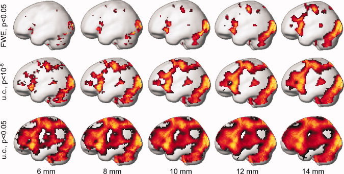
Group results (18 subjects) of the visuomotor task at different statistical thresholds (indicated on the left, u.c. = uncorrected) and filter widths (FWHM, indicated at the bottom of the figure) rendered on a standard brain surface of the left hemisphere. Each map of the t‐values was individually scaled to its maximum. [Color figure can be viewed in the online issue, which is available at wileyonlinelibrary.com.]

Figure 7.

Group results for the left hemisphere. (a) Effects of filter width on response‐peak t‐values and the number of significant peaks in the group results for probabilistically defined anatomical ROIs in the left hemisphere. Results obtained using an 8‐mm filter, i.e., the filter width most commonly used in group statistics in current fMRI studies [Breckel, 2007], are marked by a black box. All conventions as in Figure 4. (a,b): Results at a significance threshold of P < 0.05, FWE‐corrected (note that it is generally assumed that FWE correction requires filtering with at least two times the functional voxel size [Friston et al., 1996], thus the FWE‐corrected results for the unsmoothed data and filter widths of 4‐ and 5‐mm FWHM are only shown for completeness). (c) and (d): Results at a significance threshold of P < 10⁻⁵. (e) and (f): Results at a significance threshold of P < 0.05. [Color figure can be viewed in the online issue, which is available at wileyonlinelibrary.com.]

Figure 8.

Group results for the right hemisphere. (a) Effects of filter width on response‐peak t‐values and the number of significant peaks in the group results for probabilistically defined anatomical ROIs in the right hemisphere. All conventions as in Figure 7. (a,b): Results at a significance threshold of P < 0.05, FWE‐corrected. (c) and (d): Results at a significance threshold of P < 10⁻⁵. (e) and (f): Results at a significance threshold of P < 0.05. [Color figure can be viewed in the online issue, which is available at wileyonlinelibrary.com.]

In Figures 7 and 8, the results obtained using the often used 8‐mm filter width are outlined in black. In the FWE‐corrected results for the right‐ and left‐hemisphere ROIs, responses were bilaterally detected in the visual areas BA 17 and BA 18 and also—in the SMA of both hemispheres. In addition, responses in the left hemisphere were detected in the primary motor, somatosensory, and premotor areas. All these latter responses were, however, only detected using 7‐mm smoothing. Using an 8‐mm filter width, neither primary motor nor premotor responses were detected in the FWE‐corrected data. Similarly, the right primary visual cortex responses were not detected at 8‐mm smoothing (Fig. 8a), but they were detected with both narrower and broader filters (Fig. 8a,b). For narrow filters, multiple peaks were identified in the right BA 17 (Fig. 8b,d). Interestingly, the right BA 17 responses could not be recovered by lowering the statistical threshold to P < 0.05, uncorrected (Fig. 8e). A similar behavior was found in the left BA 44 (see Fig. 7), where no significant response was detected using a 7‐mm filter, even at the lowest investigated threshold (P < 0.05, Fig. 7e), but multiple peaks were found for narrower filters, and a highly significant response was evident when using broader filters.

Each of the three different types of t value traces over scales identified in the individual data sets (Figs. 4 and 5) was also present in the group data: (1) t‐value traces with maximal values in the unsmoothed data or for narrow filters (4‐ and 5‐mm FWHM) such as the left area 4p or the right BA 18; (2) t value traces with maximal values at intermediate filter widths (6‐ to 8‐mm FWHM) such as in the left SMA; and (3) t‐traces with significant values both for narrow and broad (9‐mm and above FWHM) filters, such as in the right BA 17. In addition, the left BA 17 showed increasing t values over the whole investigated range of filter widths, i.e., a type of t‐value dependence on filter width that was not observed in the individual data.

Finally, we performed an additional analysis using an alternative criterion for defining anatomical ROIs. The analyses were performed to assure that our results did not only hold for one specific ROI definition, but were more general. In our alternative definition, the ROI was restricted to the core regions of the probabilistically defined anatomical area with an anatomical assignment probability of at least 90% (see Methods). We found that the observation‐scale‐related variability was not abolished when using the anatomical core regions as ROIs for the analysis (see Fig. 9).

Figure 9.

Peak assignment to anatomical core regions of the primary and secondary visual cortex (FWE‐corrected, P < 0.05). In this analysis, we tested for observation‐scale‐related variability using an alternative criterion for definition of anatomical ROIs with assignment probability of at least 90%. In the inset, these core areas are shown on a coronal anatomical slice for the example of the primary visual (V1, green) and secondary visual (V2, red) cortex. The border areas of V1 and V2 with lower anatomical probabilities are, together, shown in black. The bar plot shows t values of all significant response peaks in V1 (green), V2 (red), and in the border region of V1 and V2 (black) in a stacked manner. [Color figure can be viewed in the online issue, which is available at wileyonlinelibrary.com.]

DISCUSSION

In the present study, we investigated scale‐related variability of the assignment of fMRI‐response peaks in a visuomotor task to cortical areas defined using a probabilistic cytoarchitectonically‐based atlas system, both for individual subjects and at a group level. According to the scale‐space framework [Iijima, 1962; Koenderink, 1984; Witkin, 1983], observation scale is determined by a spatial smoothing filter applied to imaging data. Our results clearly show that observation‐scale‐related variability can have a substantial impact on fMRI brain mapping results: depending on the observation scale, significant peaks in different constellations of cortical areas can be found. This is true for both single‐subject and group analyses, for different levels of significance (FWE‐corrected, as well as uncorrected results using both high and low statistical thresholds), for different definitions of anatomical regions of interest (ROIs), and for both small (e.g., filters below 8‐mm FWHM, Figs. 7 and 8) and large filters.

Previous studies have compared single‐filter and multi‐filter analyses, in particular for PET imaging data, in terms of their sensitivity to detect activated brain regions [e.g., Poline and Mazoyer, 1994b]. In contrast, the aim of the present study was to document the amount of variability that ensues from single‐filter analysis with different filter widths. This approach was adopted from the study by [Jones et al., 2005], who investigated observation‐scale‐related variability for VBM analyses of diffusion tensor data. Because of the different aims, there are two major methodological differences between the present study or the previous study by [Jones et al., 2005] and studies using scale search for brain responses [Crivello et al., 1995]. First, in scale search for brain responses using multi‐filter analysis, multiple statistical tests are performed for different spatial scales, these multiple tests need to be taken into account to control the false‐positive rate. To this aim, scale‐space searches have been integrated with Gaussian random field theory [Shafie et al., 2003; Siegmund and Worsley, 1995; Worsley, 2001; Worsley et al., 1996, 1997]. In contrast, in the present study, we performed correction for multiple tests only for the spatial but not for the scale domain because we aimed not to actually perform a scale search, but rather investigate the differences between typical single‐scale fMRI analyses when performed at different spatial scales, i.e., using different filter widths. Second, for scale‐space searches, logarithmic sampling of the scale dimension is optimal [Siegmund and Worsley, 1995]. In the present study, we used linearly‐spaced filter widths in order to cover the range of filters commonly used in current fMRI studies.

Generally, there are several reasons motivating spatial smoothing of fMRI data: to improve the signal‐to‐noise ratio (SNR); to fulfill Gaussian field theory requirements (i.e., to ensure that the statistical parametric maps are reasonable lattice representations of underlying continuous Gaussian fields); and to increase the overlap of individual activations in group‐level statistics [Lowe and Sorenson, 1997; Worsley et al., 1996]. The filter widths typically applied in fMRI studies range from 2‐ to 12‐mm FWHM [Breckel, 2007]. However, there are examples of fMRI studies using filters in the 12‐ to 15‐mm range [Birbaumer et al., 2005; Schlosser et al., 1998; Tyler et al., 2003; Tyler et al., 2004]. We therefore included large filter widths up to 16‐mm FWHM in the present study. The most commonly used filter width in a sample of fMRI studies was 8‐mm FWHM (used in 34.4% of studies), followed by 6‐mm FWHM (used in 23.0% of studies), while 7 mm smoothing was rarely used, i.e., only in 4.9% of studies [Breckel, 2007]. In the same study, filter widths were investigated in terms of their ratio to the voxel size of the functional data, to which the filter was applied. About 45.9% of studies used a filter width that equaled twice the voxel size of the functional data, possibly following [Friston et al., 1996] statement that the least degree of smoothing large enough to ensure the validity of the statistical inference in family‐wise error correction is twice the voxel size of the functional images.

On the basis of the results of the present study, we suggest that, in addition to the above‐mentioned statistical considerations, scale selection for fMRI studies should take into account the possibility of substantial observation‐scale‐related variability of response‐peak assignment to anatomical regions of interest. Thus, one anatomical region of interest in the present study was the primary motor cortex consisting of two subareas, Areas 4a and 4p [Geyer et al., 1996]. Previous fMRI studies assigning response peaks to the probabilistically defined Areas 4a and 4p used filter widths of 4 mm [Wilson et al., 2004], 6 mm [Sharma et al., 2008], 7 mm × 7 mm × 10 mm [Loubinoux et al., 2007], and “8–10 mm” [Binkofski et al., 2002]. Within this range of filter widths, we found different results with respect to the question in which of these two areas responses were detectable: at a statistical threshold of P < 10⁻⁵, significant peaks in the Area 4p were present for a 4‐mm filter width and in the unsmoothed data, while significant peaks in the Area 4a were present for 5‐ to 7‐mm filter widths (Fig. 7c). Thus, in this example, contradictory conclusions about the involvement of Areas 4a and 4p might have been drawn, depending on the filter width used. A similar effect was also observed in the group results where, for small filter widths, responses were found in both the right primary and secondary visual areas (BA 17 and BA 18) and in the right SMA. Using the commonly applied 8‐mm filter width, however, no significant BA 17 responses were detected, even at a low statistical threshold. BA 17 responses reappeared for large filter widths (Fig. 8a). A third, similar example was found in the left BA 44, where no responses were detectable at 7‐mm smoothing, even at a low threshold, but there were highly significant response peaks in this area both with smaller and larger filter widths (see Fig. 7). These examples illustrate that the response pattern observed in an fMRI study when using peak assignment to probabilistically‐defined anatomical areas may substantially change as a function of filter width. Such changes in the observed response pattern may lead to profoundly different functional interpretations, which points to the necessity for multi‐filter analyses. In the study on VBM analysis, [Jones et al., 2005] came to a similar conclusion. They varied filter widths from 0 to 16 mm and observed that the change of this parameter strongly influenced the results. Thus, for small‐to‐medium filter widths, significant patient‐control differences occurred in the cerebral cortex, whereas for large filter widths they were found in the cerebellum.

Interestingly, in the visuomotor data sets analyzed in this study, we did not observe any instance where, for a given anatomical ROI, significant peaks were only found for broad filters (in the FWE‐corrected visuomotor dataset), without any significant peak for narrow filters. Analysis of the auditory datasets in the present study revealed cases where, for FWE‐corrected data, significant responses could be only revealed with filter sizes =10 mm FWHM (Supporting Information Fig. 3). Therefore, there appears to be no general guarantee that restricting analyses to smaller filters will reveal all responses present in fMRI data.

The mechanisms underlying such variability may be understood through a deep‐structure analysis, as in the work by Lindeberg et al. based on gray‐level blobs parameterizing the extent of activated brain regions at each scale level [Lindeberg et al., 1999]. In this concept, the generic “blob” events in scale space are (a) annihilation, i.e., activation vanishes as scale is increased, (b) merging of multiple blobs into a single blob, (c) splitting of a single blob into multiple blobs, and (d) creation of a new blob, not present at smaller scales [Lindeberg et al., 1999]. Such scale‐space events may also explain the scale‐related variability observed in the present study. For instance, the aforementioned scale‐related variability effects in Areas 4a/4p might be explained by annihilation and creation effects in the Area 4p and 4a, respectively. Alternatively, shifts in peak location may have contributed to the observed variability of the results. Deep‐structure analyses, as by [Lindeberg et al., 1999], are a way to further investigate these different scenarios and, hence, would be an important subject for future research.

A notable aspect of the present results are the apparent discrepancies between the individual and group results, e.g., in the case of BA17 (Fig. 4 vs. Figs. 7 and 8). Alongside with the effects arising from noise spatial structure, the size and shape of fMRI responses can be expected to be the dominant factor that determines the effects of filter size on the t‐values of fMRI responses in the individual results. Inter‐individual anatomical variability is an additional factor that influences group results and refers to the size and shape of responses as well as to their exact location. A larger inter‐individual variability of response locations would require larger filter sizes to achieve spatial overlap of the individual responses. Thus, inter‐individual variability may explain the divergent results on the group level, as compared to the individual level observed in this study.

The results of the present study were obtained by assigning response peaks to probabilistically defined anatomical brain areas. A similar variability is likely to occur with other atlas systems—this would be a topic for further research. Another important further step would be to investigate observation‐scale‐related variability in studies that use not peak assignments but average responses from anatomical ROIs [e.g., Ball et al., 2007]. Furthermore, it might also be of interest to investigate to what extent the findings on scale effects in the present study generalize to other tasks and to differences between experimental conditions. Scale effects in the present study were found across a wide range of different cortical areas. We anticipate that similar effects will be also observed in other task conditions. In respect to differential contrast, it is possible that if responses in one condition were spatially more localized than in the other, the outcome of the differential contrast might critically depend on the observation scale. In an extreme case, one condition might show increased responses compared to another condition at one scale, and the other way round at another scale. Similarly, in studies comparing patient samples to healthy controls, the outcome might be scale‐dependent if the spatial extent of brain responses is influenced by pathology. A prominent example where the size of cortical representations is modulated by pathological processes and therapeutic interventions is the effect of brain lesions and that of rehabilitation training on motor representations [e.g., Eisner‐Janowicz et al., 2008; Traversa et al., 1997].

Scale‐space searches in functional brain imaging data may also allow to infer information about the extent and shape of brain responses [Poline and Mazoyer, 1994b; Shafie et al., 2003; Worsley, 2001; Worsley et al., 1996], as well as about the spatial structure of brain response maps obtained with the help of deep structure analysis [Lindeberg et al., 1999]. In the present study, both in individual and group results, we found examples where responses in probabilistically defined areas were significant when both small and large filters, but not intermediate filter widths were applied (Fig. 5c,f). This finding might be explained by the presence of local clusters of distinct cortical responses. In this case, responses are well‐detectable using either small filters that match individual small foci within a cluster, or large filters covering the entire cluster. At some intermediate scales, however, the size of the filter would match neither the fine activations nor the result of their merges. Such an effect might lead to wrong results—or absence of results—with single‐scale studies. Similarly, visual stimulation‐related fMRI responses have been previously detected over a broad range of scales by Worsley et al. This was interpreted as a presence of a cluster with sharp foci embedded in a “penumbra” of lesser activation [Worsley, 2001]. Alternatively, analyses with small filter widths might be biased toward signals from draining veins [Nencka and Rowe, 2007; Turner, 2002], as narrow filters of only few‐mm FWHMs could be expected to match the similar diameter of draining veins better, as compared to broad filters. It is therefore unclear whether our results are due to a spatial organization principle of brain responses or, alternatively, they are influenced by vascular effects. We anticipate that further research into this direction might particularly profit from restricting scale‐space searches to the cortical surface as proposed by [Andrade et al., 2001] using cortically constrained 2D filters to avoid partial volume effects with the adjacent white matter or draining veins. Such analyses might eventually reveal novel spatial organization principles of neuronal activity in the human cerebral cortex.

Practical Consequences

By demonstrating substantial observation‐scale‐related variability of fMRI response maps, our findings strongly emphasize the importance of multi‐scale methods as suggested and elaborated in a series of previous studies [Coulon et al., 2000; Lindeberg et al., 1999; Poline and Mazoyer, 1994a, b; Worsley, 2001; Worsley et al., 1996, 1997]. Alongside with previous work on scale‐space analyses, our study may encourage the implementation of methods for scale‐space searches and of reliable multiple comparison methods for scale‐space analyses in existing fMRI software packages. Such a valuable addition would facilitate widespread application of these methods by the fMRI community. Owing to theoretical groundwork laid during the last decades, such an implementation is likely to face no substantial obstacles other than the time and effort required.

Our findings indicate that the range of useful filter widths to be considered for scale selection in fMRI brain mapping appears to be broader than previously assumed. In many cases, large filter widths resulted in maximal t values within anatomical ROIs in the present study. Our results indicate that it is generally useful to check whether results obtained with a single filter size also hold with other filter sizes. In practice, the range of useful filter sizes may be limited by the spatial scale of the anatomical target structures of a study—such as to small filters for investigation of small subcortical nuclei. For analysis of cortical responses, it might be especially useful to combine scale‐space approaches with cortically constrained analyses/filtering [Andrade et al., 2001; Chung et al., 2005; Operto et al., 2008]. 3D filters merge gray and white matter voxels—a particularly important problem using larger 3D filters. Therefore, cortically constrained filtering can be expected to be practically useful to gain the full advantage of scale‐space searches for exploring the spatial structure of activity in the cerebral cortex.

Supporting information

Additional Supporting Information may be found in the online version of this article.

Supplementary Figure 1: To determine the behavior of t‐values over scales, i.e. filter sizes, the following procedure was used as illustrated in the figure where an anatomical region of interest (ROI) is schematically displayed with significant responses peaks symbolized by asterices. For each filter size, then the maximum of the t‐values corresponding to the significant peaks in the ROI was determined and these values were then rendered in a color coded way. Supplementary Figure 2: Dependence of voxelwise t‐values on filter width for the responses in the auditory cortex regions obtained during presentation of short piano pieces as auditory stimuli. Conventions as in Fig. 2 of the main manuscript. Supplementary Figure 3: Group results for the left hemisphere. Effects of filter width on response‐peak t‐values and the number of significant peaks in the group results of the music‐related responses for probabilistically defined anatomical ROIs in the left hemisphere. Conventions as in Fig. 7 of the main manuscript.

REFERENCES

- Amunts K, Schleicher A, Burgel U, Mohlberg H, Uylings HB, Zilles K ( 1999): Broca's region revisited: Cytoarchitecture and intersubject variability. J Comp Neurol 412: 319–341. [DOI] [PubMed] [Google Scholar]
- Amunts K, Schleicher A, Ditterich A, Zilles K ( 2003): Broca's region: Cytoarchitectonic asymmetry and developmental changes. J Comp Neurol 465: 72–89. [DOI] [PubMed] [Google Scholar]
- Andrade A, Ferath K, Mangin D, Bihan D, Poline JB ( 2001): Scale space searches in cortical surface analysis of fMRI data. Neuroimage 13: 1290. [Google Scholar]
- Ball T, Rahm B, Eickhoff SB, Schulze‐Bonhage A, Speck O, Mutschler I ( 2007): Response properties of human amygdala subregions: Evidence based on functional MRI combined with probabilistic anatomical maps. PLoS One 2: e307. [DOI] [PMC free article] [PubMed] [Google Scholar]
- Binkofski F, Fink GR, Geyer S, Buccino G, Gruber O, Shah NJ, Taylor JG, Seitz RJ, Zilles K, Freund HJ ( 2002): Neural activity in human primary motor cortex areas 4a and 4p is modulated differentially by attention to action. J Neurophysiol 88: 514–519. [DOI] [PubMed] [Google Scholar]
- Birbaumer N, Veit R, Lotze M, Erb M, Hermann C, Grodd W, Flor H ( 2005): Deficient fear conditioning in psychopathy: A functional magnetic resonance imaging study. Arch Gen Psychiatry 62: 799–805. [DOI] [PubMed] [Google Scholar]
- Breckel T ( 2007): Scale‐Space Variability of Visuomotor Functional MRI Responses. Freiburg: Albert‐Ludwigs‐Universität. [Google Scholar]
- Choi HJ, Zilles K, Mohlberg H, Schleicher A, Fink GR, Armstrong E, Amunts K ( 2006): Cytoarchitectonic identification and probabilistic mapping of two distinct areas within the anterior ventral bank of the human intraparietal sulcus. J Comp Neurol 495: 53–69. [DOI] [PMC free article] [PubMed] [Google Scholar]
- Chung MK, Robbins SM, Dalton KM, Davidson RJ, Alexander AL, Evans AC ( 2005): Cortical thickness analysis in autism with heat kernel smoothing. Neuroimage 25: 1256–1265. [DOI] [PubMed] [Google Scholar]
- Coulon O, Bloch I, Froulin V, Mangin J‐F ( 1997): Multiscale measures in linear scale‐space for characterizing cerebral functional activations in 3D PET difference In: Romney B, Florack L, Koenderink JJ, Viergever M, editors. ScaleSpace'97, LNCS vol. 1252, Utrecht: Springer‐Verlag; pp 188–199. [Google Scholar]
- Coulon O, Mangin JF, Poline JB, Zilbovicius M, Roumenov D, Samson Y, Frouin V, Bloch I ( 2000): Structural group analysis of functional activation maps. Neuroimage 11: 767–782. [DOI] [PubMed] [Google Scholar]
- Crivello F, Tzourio N, Poline JB, Woods RP, Mazziotta JC, Mazoyer B ( 1995): Intersubject variability in functional neuroanatomy of silent verb generation: Assessment by a new activation detection algorithm based on amplitude and size information. Neuroimage 2: 253–263. [DOI] [PubMed] [Google Scholar]
- Eickhoff SB, Stephan KE, Mohlberg H, Grefkes C, Fink GR, Amunts K, Zilles K ( 2005): A new SPM toolbox for combining probabilistic cytoarchitectonic maps and functional imaging data. Neuroimage 25: 1325–1335. [DOI] [PubMed] [Google Scholar]
- Eisner‐Janowicz I, Barbay S, Hoover E, Stowe AM, Frost SB, Plautz EJ, Nudo RJ ( 2008): Early and late changes in the distal forelimb representation of the supplementary motor area after injury to frontal motor areas in the squirrel monkey. J Neurophysiol 100: 1498–1512. [DOI] [PMC free article] [PubMed] [Google Scholar]
- Florack L, ter Haar Romney BM, Koenderink JJ ( 1992): Scale‐space and the differential structure of images. Image Vis Comput 10: 376–388. [Google Scholar]
- Fransson P, Merboldt KD, Petersson KM, Ingvar M, Frahm J ( 2002): On the effects of spatial filtering—A comparative fMRI study of episodic memory encoding at high and low resolution. Neuroimage 16: 977–984. [DOI] [PubMed] [Google Scholar]
- Friston KJ, Holmes A, Poline JB, Price CJ, Frith CD ( 1996): Detecting activations in PET and fMRI: Levels of inference and power. Neuroimage 4: 223–235. [DOI] [PubMed] [Google Scholar]
- Geissler A, Lanzenberger R, Barth M, Tahamtan AR, Milakara D, Gartus A, Beisteiner R ( 2005): Influence of fMRI smoothing procedures on replicability of fine scale motor localization. Neuroimage 24: 323–331. [DOI] [PubMed] [Google Scholar]
- Geyer S, Ledberg A, Schleicher A, Kinomura S, Schormann T, Burgel U, Klingberg T, Larsson J, Zilles K, Roland PE ( 1996): Two different areas within the primary motor cortex of man. Nature 382: 805–807. [DOI] [PubMed] [Google Scholar]
- Iijima T ( 1962): Basic theory of pattern normalization (for the case of a typical one dimensional pattern). Bull Electrotechn Lab (in Japanese) 26: 368–388. [Google Scholar]
- Jones DK, Symms MR, Cercignani M, Howard RJ ( 2005): The effect of filter size on VBM analyses of DT‐MRI data. Neuroimage 26: 546–554. [DOI] [PubMed] [Google Scholar]
- Koenderink JJ ( 1984): The structure of images. Biol Cybern 50: 363–370. [DOI] [PubMed] [Google Scholar]
- Kuijper A, Florack LJ ( 2003): The hierarchical structure of images. IEEE Trans Image Process 12: 1067–1079. [DOI] [PubMed] [Google Scholar]
- Lindeberg T ( 1994): Scale‐Space Theory in Computer Vision. Dordrecht: Kluwer Academic Publishers. [Google Scholar]
- Lindeberg T ( 1999): Automatic Scale Selection as a Pre‐Processing Stage for Interpreting the Visual World In: Chetverikov D. and Sziranyi T, editors. Proc. FSPIPA, vol. 130, Budapest: Schriftenreihen der Österreichischen Computer Gesellschaft; p 9–23. [Google Scholar]
- Lindeberg T, Lidberg P, Roland PE ( 1999): Analysis of brain activation patterns using a 3‐D scale‐space primal sketch. Hum Brain Mapp 7: 166–194. [DOI] [PMC free article] [PubMed] [Google Scholar]
- Loubinoux I, Dechaumont‐Palacin S, Castel‐Lacanal E, De BX, Marque P, Pariente J, Albucher JF, Berry I, Chollet F ( 2007): Prognostic value of FMRI in recovery of hand function in subcortical stroke patients. Cereb Cortex 17: 2980–2987. [DOI] [PubMed] [Google Scholar]
- Lowe MJ, Sorenson JA ( 1997): Spatially filtering functional magnetic resonance imaging data. Magn Reson Med 37: 723–729. [DOI] [PubMed] [Google Scholar]
- Marsden CD, Deecke L, Freund HJ, Hallett M, Passingham RE, Shibasaki H, Tanji J, Wiesendanger M ( 1996): The functions of the supplementary motor area. Summary of a workshop. Adv Neurol 70: 477–487. [PubMed] [Google Scholar]
- Mutschler I ( 2007): The role of the human amygdala and insular cortex in emotional processing: Investigationsusing functional MRI combined with probabilistic anatomical maps. Digital dissertation. Eberhard Karls Universität Tübingen: http://nbn-resolving.de/urn:nbn:de:bsz:21-opus-29817.
- Mutschler I, Wieckhorst B, Speck O, Schulze‐Bonhage A, Hennig J, Seifritz E, Ball T ( 2010): Time scales of auditory habituation in the amygdala and cerebral cortex. Cereb Cortex 20: 2531–2539. [DOI] [PubMed] [Google Scholar]
- Nencka AS, Rowe DB ( 2007): Reducing the unwanted draining vein BOLD contribution in fMRI with statistical post‐processing methods. Neuroimage 37: 177–188. [DOI] [PubMed] [Google Scholar]
- Oldfield RC ( 1971): The assessment and analysis of handedness: The Edinburgh inventory. Neuropsychologia 9: 97–113. [DOI] [PubMed] [Google Scholar]
- Operto G, Clouchoux C, Bulot R, Anton JL, Coulon O ( 2008): Surface‐based structural group analysis of fMRI data. Med Image Comput Comput Assist Interv 11: 959–966. [DOI] [PubMed] [Google Scholar]
- Poline JB, Mazoyer BM ( 1994a): Analysis of individual brain activation maps using hierarchical description and multiscale detection. IEEE Trans Med Imaging 13: 702–710. [DOI] [PubMed] [Google Scholar]
- Poline JB, Mazoyer BM ( 1994b): Enhanced detection in brain activation maps using a multifiltering approach. J Cereb Blood Flow Metab 14: 639–642. [DOI] [PubMed] [Google Scholar]
- Ridgway GR, Henley SM, Rohrer JD, Scahill RI, Warren JD, Fox NC ( 2008): Ten simple rules for reporting voxel‐based morphometry studies. Neuroimage 40: 1429–1435. [DOI] [PubMed] [Google Scholar]
- Rosbacke M, Lindeberg T, Bjorkman E, Roland PE ( 2001): Evaluation of using absolute versus relative base level when analyzing brain activation images using the scale‐space primal sketch. Med Image Anal 5: 89–110. [DOI] [PubMed] [Google Scholar]
- Rosenfeld A Kak AC ( 1982): Digital Picture Processing. Orlando: Academic Press. [Google Scholar]
- Schenker NM, Buxhoeveden DP, Blackmon WL, Amunts K, Zilles K, Semendeferi K ( 2008): A comparative quantitative analysis of cytoarchitecture and minicolumnar organization in Broca's area in humans and great apes. J Comp Neurol 510: 117–128. [DOI] [PubMed] [Google Scholar]
- Schlosser R, Hutchinson M, Joseffer S, Rusinek H, Saarimaki A, Stevenson J, Dewey SL, Brodie JD ( 1998): Functional magnetic resonance imaging of human brain activity in a verbal fluency task. J Neurol Neurosurg Psychiatry 64: 492–498. [DOI] [PMC free article] [PubMed] [Google Scholar]
- Shafie K, Sigal B, Siegmund DO, Worsley KJ ( 2003): Rotation space random fields with an application to fMRI data. Ann Stat 31: 1732–1771. [Google Scholar]
- Sharma N, Jones PS, Carpenter TA, Baron JC ( 2008): Mapping the involvement of BA 4a and 4p during Motor Imagery. Neuroimage 41: 92–99. [DOI] [PubMed] [Google Scholar]
- Siegmund DO, Worsley KJ ( 1995): Testing for a signal with unknown location and scale in a stationary gaussian random field. Ann Stat 23: 608–639. [Google Scholar]
- Thesen S, Heid O, Mueller E, Schad LR ( 2000): Prospective acquisition correction for head motion with image‐based tracking for real‐time fMRI. Magn Reson Med 44: 457–465. [DOI] [PubMed] [Google Scholar]
- Toga AW, Thompson PM, Mori S, Amunts K, Zilles K ( 2006): Towards multimodal atlases of the human brain. Nat Rev Neurosci 7: 952–966. [DOI] [PMC free article] [PubMed] [Google Scholar]
- Traversa R, Cicinelli P, Bassi A, Rossini PM, Bernardi G ( 1997): Mapping of motor cortical reorganization after stroke. A brain stimulation study with focal magnetic pulses. Stroke 28: 110–117. [DOI] [PubMed] [Google Scholar]
- Turner R ( 2002): How much cortex can a vein drain? Downstream dilution of activation‐related cerebral blood oxygenation changes. Neuroimage 16: 1062–1067. [DOI] [PubMed] [Google Scholar]
- Tyler LK, Stamatakis EA, Dick E, Bright P, Fletcher P, Moss H ( 2003): Objects and their actions: Evidence for a neurally distributed semantic system. Neuroimage 18: 542–557. [DOI] [PubMed] [Google Scholar]
- Tyler LK, Bright P, Fletcher P, Stamatakis EA ( 2004): Neural processing of nouns and verbs: The role of inflectional morphology. Neuropsychologia 42: 512–523. [DOI] [PubMed] [Google Scholar]
- Van Hecke W, Sijbers J, De Backer S, Poot D, Parizel PM, Leemans A ( 2009): On the construction of a ground truth framework for evaluating voxel‐based diffusion tensor MRI analysis methods. Neuroimage 46: 692–707. [DOI] [PubMed] [Google Scholar]
- White T, O'Leary D, Magnotta V, Arndt S, Flaum M, Andreasen NC ( 2001): Anatomic and functional variability: The effects of filter size in group fMRI data analysis. Neuroimage 13: 577–588. [DOI] [PubMed] [Google Scholar]
- Wilson SM, Saygin AP, Sereno MI, Iacoboni M ( 2004): Listening to speech activates motor areas involved in speech production. Nat Neurosci 7: 701–702. [DOI] [PubMed] [Google Scholar]
- Witkin AP ( 1983): Scale‐Space Filtering. Proc. 8th Int. Joint Conf. Art. Intell., Karlsruhe, Germany. pp 1019–1022.
- Worsley KJ ( 2001): Testing for signals with unknown location and scale in a ÷2 random field, with an application to fMRI. Adv Appl Prob 33: 773–793. [Google Scholar]
- Worsley KJ, Marrett S, Neelin P, Evans AC ( 1996): Searching scale space for activation in PET images. Hum Brain Mapp 4: 74–90. [DOI] [PubMed] [Google Scholar]
- Worsley KJ, Wolforth M, Evans AC ( 1997): Scale space searches for a periodic signal in fMRI data with spatially varying hemodynamic response. Conference paper. Proceedings of BrainMap'95: http://www.math.mcgill.ca/keith/sanant/sanant.pdf.
- Zaitsev M, Hennig J, Speck O ( 2004): Point spread function mapping with parallel imaging techniques and high acceleration factors: Fast, robust, and flexible method for echo‐planar imaging distortion correction. Magn Reson Med 52: 1156–1166. [DOI] [PubMed] [Google Scholar]
Associated Data
This section collects any data citations, data availability statements, or supplementary materials included in this article.
Supplementary Materials