A mutual information‐based metric for evaluation of fMRI data‐processing approaches

Abstract

We propose a novel approach for evaluating the performance of activation detection in real (experimental) datasets using a new mutual information (MI)‐based metric and compare its sensitivity to several existing performance metrics in both simulated and real datasets. The proposed approach is based on measuring the approximate MI between the fMRI time‐series of a validation dataset and a calculated activation map (thresholded label map or continuous map) from an independent training dataset. The MI metric is used to measure the amount of information preserved during the extraction of an activation map from experimentally related fMRI time‐series. The processing method that preserves maximal information between the maps and related time‐series is proposed to be superior. The results on simulation datasets for multiple analysis models are consistent with the results of ROC curves, but are shown to have lower information content than for real datasets, limiting their generalizability. In real datasets for group analyses using the general linear model (GLM; FSL4 and SPM5), we show that MI values are (1) larger for groups of 15 versus 10 subjects and (2) more sensitive measures than reproducibility (for continuous maps) or Jaccard overlap metrics (for thresholded maps). We also show that (1) for an increasing fraction of nominally active voxels, both MI and false discovery rate (FDR) increase, and (2) at a fixed FDR, GLM using FSL4 tends to extract more voxels and more information than SPM5 using the default processing techniques in each package. Hum Brain Mapp, 2011. © 2010 Wiley‐Liss, Inc.

INTRODUCTION

In functional magnetic resonance imaging (fMRI), the images undergo statistical analysis to localize sources of activation within the brain. Many analysis techniques are available to generate a statistical parametric map (SPM), which shows the significance (existence) of task‐dependent blood‐oxygen‐level‐dependent (BOLD) changes in each voxel of the brain. Different methods generate different maps requiring that their performance be measured to choose the optimal processing strategy.

A standard tool for evaluating the performance of activation detection methods is the receiver‐operating characteristic (ROC) curve, which can be estimated using a simulated fMRI dataset where truly active voxels are known. However, simulated datasets may not reflect all aspects of real datasets and therefore produce analysis results that are biased. Hence, performance measurement using real‐world datasets may be preferable to the standard ROC.

Several such methods estimate a reliability metric by measuring the agreement between SPMs from independent repetitions of an fMRI experiment. Strother et al. [ 1997] and Tegeler et al. [ 1999] propose a single summary metric of whole‐brain pattern reproducibility for pairs of SPMs from independent datasets. Machielsen et al. [ 2000] measured the reliability of a visual encoding task based on the ratio of overlapping detected areas. McGonigle et al. [ 2000] compared the detected areas calculated from a single session, fixed‐effect analysis and mixed‐effect analysis and showed that for single session analysis of repeated sessions erroneous conclusions are possible. Genovese et al. [ 1997] and Maitra et al. [ 2002] estimate a pseudo‐ROC curve and a reliability map from SPMs of repeated trials of an fMRI experiment, based on a multinomial model of individual voxels (see also Gullapalli et al. [ 2005]). Chen and Small [ 2007] estimated pseudo‐ROC curves of multiple linear regression analysis applied to the datasets of stroke patients and healthy participants. The pseudocurve approach is implemented by obtaining a test statistic and thresholding it at different levels. Maitra [ 2009] reformulated the problem to eliminate the thresholding requirement.

Reliability of fMRI results is also measured using the intraclass correlation coefficient (ICC) of a number of SPMs [Raemaekers et al., 2007; Shrout and Fleiss, 1979]. Friedman et al. [ 2008] estimated between‐site reliability of an fMRI experiment using ICC. Sprecht et al. [ 2003] used a voxelwise ICC, correlation coefficient of contrast t‐values for pairs of activation maps, and the ratio of overlapping detected areas to assess the reliability of a functional imaging study. Wei et al. [ 2004] calculated the within‐subject ICC and between‐subject ICC for some regions of interest and compared them.

In addition to reliability measures for continuous SPMs, there are measures for voxel‐label maps produced by thresholding an SPM and labeling voxels as active or nonactive. Le and Hu [ 1997] performed a reliability assessment of binary maps using the “Kappa” statistic [Cohen, 1960]. Other measures of common agreement are the simple matching coefficient, the Jaccard coefficient [JC; Jaccard, 1901], and the Dice coefficient [DC; Dice, 1945]. DC has been commonly used for evaluation in functional neuroimaging [Raemaekers et al., 2007; Rombouts et al., 1998] and has been shown to be asymptotically related to the kappa statistic [Frackowiak et al., 2004; Zijdenbos et al., 2002]. DC tends to overstate the degree of overlap, which is given directly by JC as the ratio of intersection/union of thresholded voxels, with DC = 2JC/(JC + 1) [Shattuck et al., 2001]. A generalization of the JC is proposed by Maitra [ 2010] to summarize the reliability of multiple fMRI studies. For a comprehensive review of reliability metrics of binary maps, see Colwell and Coddington [ 1994] and Ruddell et al. [ 2007]. For measurement of reliability in general medical informatics studies, see Hripcsak and Heitjanb [ 2002].

All the abovementioned evaluation techniques measure common agreement between the SPMs or label maps calculated from independent datasets of the same task. The processing method that generates more similar SPMs will generate a larger area under its pseudo‐ROC curve or a larger reproducibility/reliability metric using the test–retest approach. These methods are unable to detect a consistent, model‐dependent bias because they assume that fMRI analysis techniques are making only random, independent errors across independent datasets. For example, a method that always declares some voxels as active independent of the input dataset will have maximum reliability but very low accuracy. While an extreme example, all models will have some, possibly spatially dependent bias that will remain undetected in finite samples using parameter estimation.

Other evaluation approaches provide the relative ranks of the analysis techniques under evaluation. Williams' index [Williams, 1976] uses a user‐defined similarity measure (e.g., JC, DC, kappa, ICC, etc.) to compare label or continuous maps. The analysis techniques are ranked by their degrees of similarity to other methods. The method more similar to the other methods gets the best rank. Multidimensional scaling [MDS; Borg and Groenen, 2005; Bouix et al., 2007; Cox and Cox, 1994] is a visualization technique that shows the relative distance of several analysis techniques as well as their reliabilities on a 2D graph. The distance is measured by any of the similarity measures mentioned above. STAPLE is a technique developed by Warfield et al. [ 2004] to measure the relative quality of multilabel maps from different analysis techniques with a reference standard through an expectation maximization framework. The methods are ranked by their similarity to the estimated reference. To calculate the reference, STAPLE assumes different analysis techniques make independent errors, which is not necessarily true. Generally, if a method outperforms others and uniquely detects a correct brain region, this method might not be rated the best. Therefore, an evaluation approach that provides an individual metric for each method might be more useful (see Bouix et al. [ 2007] for a comparison of Williams' index, STAPLE, and MDS).

Another category of evaluation methods measure the prediction or generalization error of both labeled and unlabeled datasets using a model [Hansen et al., 1999; LaConte et al., 2005; Mørch et al., 1997; Strother et al., 2002]. These evaluation methods divide a dataset into training and test sets and fit a model to the training set. Some hyperparameters of the fitted training model are then tuned to best predict the known scan labels or the probability density of the test dataset. The label prediction error depends on how the training set model parameters generalize to the test set. These measures may or may not reflect the quality of preprocessing approaches that remove artifacts and noise from the datasets [Chen et al., 2006; LaConte et al., 2003; Strother et al., 2004; Zhang et al., 2008].

The NPAIRS method [Kjems et al., 2002; Strother et al., 2002; Zhang et al., 2008] uses both reproducibility and prediction metrics for quantitative evaluation of neuroimage analysis techniques by simultaneously measuring test–retest spatial pattern reproducibility and temporal prediction. They argue that the prediction versus reproducibility curve can capture the bias‐variance trade off of a model. This approach has been extended, to include a second‐level canonical variates analysis (CVA) for comparing single‐subject processing pipelines [LaConte et al., 2003; Zhang et al., 2009], and to allow comparison of non‐linear BOLD hemodynamic models estimated in a Bayesian framework using Markov Chain Monte Carlo techniques with a Kullback‐Leibler measure to estimate reproducibility [Jacobsen et al., 2008].

We propose a new performance evaluation approach for analysis techniques that analytically links the spatial SPM and experimentally related temporal structures across independent datasets (i.e, crossvalidation training and test sets) with a single mutual information (MI) metric. MI generalizes the concept of a relationship between two random variables from only linear Gaussian relationships captured by a correlation coefficient to arbitrary nonlinear associations between Gaussian and non‐Gaussian variables. In the Appendix we show the relationship between Shannon entropy, which measures the amount of uncertainty or lack of information of a variable [see Eq. (A1)], and MI. Using this relationship involving the uncertainty in random variables x and y, MI may be described as the amount of uncertainty in x that is removed, or the information gained about x, by knowing y, or vice‐versa (see the first paragraph under Methods section to know about the bold formatting for variables mentioned in this sentence). Our approach evaluates fMRI pipelines by assuming that the data analysis goal is to produce a label map, or a continuous SPM, with a quantifiable relationship to the clustering/ordering of voxel‐based time‐series. This relationship is quite likely to involve a nonlinear dependence between non‐Gaussian variables requiring the use of MI. This new MI technique may be viewed as creating a formal analytic link between the prediction (experimental temporal domain) and reproducibility (spatial agreement) metrics of the NPAIRS approach.

METHODS

In the following text and equations, bold variables (e.g., y, s, c) are random vectors (or variables) and normal variables with subscript i (e.g., y _i, s _i, c _i) are the time‐series or the calculated statistic of voxel i.

Theory

Assume a fMRI dataset consists of p scans of N intracerebral voxels with the notation y _i for a p‐dimensional vector of the time‐series of voxel i (1 ≤ i ≤ N) throughout the article. A fMRI processing approach (f) compresses the time‐series of voxel i (y _i) into a statistic [s _i = f(y _i)], which can be thresholded using a function (g) to generate a binary label [c _i = g(s _i)] showing whether the voxel i is detected as active (c _i = 1) or nonactive (c _i = 0). The binary map (c _i) typically depends on the threshold value we choose in function g. This threshold value depends on the distribution and dynamic range of the statistic (s _i), which might be different for different analysis techniques. Therefore, instead of a threshold value, we use the relative number of voxels declared active γ = to show the dependence of the binary map on the chosen threshold. We assume that the time‐series of each voxel is an observation of a random vector y, the estimated statistics of each voxel is an observation of a random variable s, and the estimated voxels' labels are observations of a random variable c with P{c = 1} = γ where distributions are unknown and may vary across voxels. If at least two independent repetitions of an experiment (e.g., repeat runs within a scanning session, repeat sessions for a subject, or multiple subjects) that are spatially aligned are available (this is extended to more than two datasets later in the article), we call one of them the training dataset (y ^t) and the other the validation dataset (y ^v). Therefore, using information inequality, one can write [Cover and Thomas, 1991]

(1)

where I(.,.) is any measure of information between two random variables or vectors. We calculate the MI between a continuous random variable s ^t and a random vector y ^v based on the Kullback–Leibler divergence between the joint probability density function P(s ^t, y ^v) and the product of their marginal probability density functions P(s ^t)P(y ^v):

(2)

The MI between a binary random variable c ^t and random vector y ^v may also be calculated based on the Kullback–Leibler divergence between the joint probability density function P(c ^t, y ^v) and the product of their marginal probability density functions P(c ^t)P(y ^v), which is defined as follows:

(3)

If the goal is to evaluate a processing method that provides a continuous map, we can use MI_CONTINUOUS = I(s ^t, y ^v) as a measure of performance. Below we describe how we do this by measuring how much generalizable information of the similarity ordering of training time‐series data y ^t is preserved in the interval ordering of voxels in the SPM s ^t. In the case that the goal is to evaluate analysis techniques that provide a label for each voxel, we can use MI_BINARY = I(c ^t, y ^v). We do this by measuring how well the labels (c ^t) reflect separate clusters in the independent temporal data (y ^v). For most analysis techniques, f generates a continuous SPM that may be transformed to a label map by thresholding the SPM. MI_BINARY measures the match between the thresholded voxel clusters from the SPM and the related separating boundary between temporal clusters in the validation set. Furthermore, we may plot I(c ^t, y ^v) = versus γ to choose an optimal threshold setting, which is a normalized variable that does not depend on the dynamic range of the SPM.

Estimating the MI Metric

In fMRI experiments, more than 100 scans (i.e., p time samples > 100) in each run are often acquired. Computing MI in such a high‐dimensional space is infeasible because it is difficult to compute the integral in a moderate‐dimensional continuous space based on limited numbers of samples [(x _i,y _i), i = 1,…,N]. Here x _i can be a binary label (c _i) or a statistic (s _i) and y _i is the time‐series of the validation dataset. Therefore, a dimension reduction algorithm is required before even approximate estimation of the MI. Our goal here is not accurate estimation of the true MI as it is unlikely that this is possible given such high‐dimensional temporal spaces. However, we show that a sensitive approximation to MI changes may be obtained using the techniques outlined below.

There are many approaches in the literature for the estimation of MI that are applicable to our problem [Blinnikov and Moessner, 1998; Cellucci et al., 2005; Darbellay and Vajda, 1999; Daub et al., 2004; Khan et al., 2007; Moon et al., 1995; Paninski, 2003]. In fMRI datasets, usually a small number of voxels are active, located in the tails of the probability density functions (pdf) of x, y, and (x,y). Therefore, a MI estimation method must reliably estimate the tails in the pdf(s) where only a few observations (active voxels) are available. Kraskov et al. [ 2004] have proposed an algorithm for MI estimation based on k‐nearest neighbor pdf estimation that is known to perform reliably in the pdf locations where only a few observations (i.e., active voxels) are available. By using some assumptions about fMRI time‐series, we have modified the Kraskov et al. [ 2004] algorithm to combine dimension reduction and MI estimation into one step. We briefly discuss the proposed method below with further details in the Appendix.

Assume X and Y are two subspaces, and the MI between their two random vectors (or variables) x and y is desired using distance measures defined as d _x(x _i,x _j) and d _y(y _i,y _j). Here, x _i and x _j are two observations of x in X and y _i and y _j are two observations of y in Y. The space Z is defined as Z = (X, Y) and the distance measure in Z is defined as

(4)

Here, theoretically, any distance metrics can be used for d _x and d _y, but only a few may be useful for approximate estimation of MI.

For every voxel i, rank d _z(z _i, z _j) from smallest to largest. Then denote ε_z(i) as the distance from z _i to its kth neighbor where the kth neighbor is defined as the voxel with the kth smallest d _z(z _i, z _j) value in the list. In the k‐nearest‐neighbor‐based estimation algorithm for MI, we count the number n _x(i) of points x _j whose distances from x _i are strictly less than ε_z(i), and similarly for y instead of x as illustrated in Figure 1. The estimate for MI is then

(5)

where N is the number of observations (time‐series) indexed by i and ψ is the digamma function, ψ(α)= Γ(α)⁻¹ dΓ(α)/dα. It satisfies the recursion ψ(α + 1) = ψ(α) + 1/α and ψ(1) = −C, where C ≈ 0.5772156 is the Euler–Mascheroni constant [Davis, 1972]. The performance of Eq. (5) for estimating MI was systematically studied by Kraskov et al. [ 2004]. This algorithm estimates the Shannon entropy of x, y, and (x, y) and then estimates MI by calculating the sum of the estimated Shannon entropy of x and y followed by subtracting the estimated Shannon entropy of (x, y) (see Appendix for a brief review of the algorithm with related pseudocode).

Figure 1.

Assessing the neighborhood size and the estimation of n _x(i) and n _y(i) in the k‐nearest neighbor‐based MI algorithm for k = 1. Left panel: The distance of the voxel i from other voxels in both validation time‐series space (d _y(y _i,y _j)) and training SPM space (d _x(x _i,x _j)) is calculated. The distance in the joint space (d _z) is defined as the maximum of the distance in the time‐series space (d _y) and the distance in the SPM statistic space (d _x). For voxel i rank d _z from smallest to largest. Then denote ε_z(i) as the distance from z _i to its kth neighbor where the kth neighbor is defined as the voxel with the kth smallest d _z(z _i,z _j) value in the list. The voxel l is the first nearest voxel to the voxel i, and for k = 1, its distance from the voxel i defines the neighborhood size; therefore, ε_z(i) = 1.7. Right panel: n _x(i) is defined as the number of voxels whose distances from voxel i in statistic space (X) is equal to or less than ε_z(i), which is n _x(i) = 3 in this example. n _y(i) is the number of voxels whose distances from voxel i in time‐series space (Y) is equal to or less thanε_z(i), which is n _y(i) = 5 in this example. For each voxel (i = 1, …, N), its kth nearest voxel is found, ε_z(i)is estimated, and using the calculated values of n _x(i) and n _y(i) the MI between the validation time‐series and SPM is estimated (see main text and Appendix for details).

As shown in Eqs. (4) and (5), the MI estimator only depends on the relative distance of the observations in X and Y space. As the X space (x _i is the estimated statistic or label for voxel i) is a one‐dimensional space, we use d _x(x _i, x _j) = |x _i − x _j| (|x| stands for the absolute value of x).

With careful choice of the distance metric in the Y space, we may combine the dimension reduction and MI estimation in one step. In the original algorithm proposed by Kraskov et al. [ 2004], the max norm is used as a distance function in time‐series space (Y) , where t is the index for the dimensions of (Y)^t. Using the max norm in time‐series space, the search space for the k nearest‐neighbor of the voxel i is the p‐dimensional time‐series and the one‐dimensional SPM space. Therefore, the estimated distance of voxel i from its k‐nearest neighbors in the joint space (ε_z(i)) will not be robust and MI estimation will have a very large variance in such a high‐dimensional space (see Results). Instead, we assume that the connection between the time‐series of voxels can be based on the idea from the literature for time‐series clustering that active voxels will tend to have larger correlations with other active voxels compared to nonactive voxels. Therefore, a correlation coefficient‐based distance function is used to define the similarity between time‐series of different voxels. 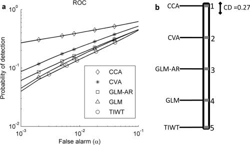A correlation‐based metric can be used to form a hyperbolic distance measure , where ρ_ij is the correlation coefficient between two time‐series (y _i, y _j). This distance measure has been shown to be robust to noise in fMRI applications [Golay et al., 1998; Gomez‐Laberge et al., 2008]. The hyperbolic distance measure reduces the dimensions of the kth nearest neighbor search space to two dimensions while ignoring possible nonlinear connections between the voxels. To calculate ρ_ij, we used those segments of the time‐series where the subject was performing the task of interest together with its adjacent fixation segments. This removed the effects of other tasks.

Figure 1 shows the MI estimation algorithm for k = 1 in the 2D joint space of validation time‐series distance and training SPM distance. The k‐nearest neighbor of voxel i is evaluated in the 2D space instead of a p + 1‐dimension space. The MI increases when n _x(i) and n _y(i) are minimum [see Eq. (5)]. If voxels have the same neighbors in the validation time‐series space and training SPM space, MI increases, and if they have different neighbors in the validation time‐series and training SPM spaces, the MI will decrease.

If several validation (sessions) fMRI datasets (1, …, Q) are available (i.e., y ${}^{\text{v}{}_{\text{1}}}$,…,y ${}^{\text{v}{}_{\mathit{\text{Q}}}}$), we first calculate the correlation coefficient between time‐series in a single dataset and then calculate the average correlation coefficient over the Q validation datasets . Therefore, the hyperbolic distance measure becomes . This averaging helps decrease the variance of MI estimation and consequently increases the sensitivity of the MI metric.

Computing and Testing MI Versus Other Performance Metrics

Assume that M independent datasets of an fMRI experiment are available, denoted by random vectors y ⁽¹⁾,…,y ^(M). The datasets are preprocessed including motion correction and registration to a common atlas. The goal is to evaluate a processing method, f or g, that maps T training datasets (1 ≤ T < M) to a single second‐level SPM (s ^t = f(y ${}^{\text{t}{}_{\text{1}}}$,…,y ${}^{\text{t}{}_{\mathit{\text{T}}}}$)) or a label map (c ^t = g(s ^t)), using Q = M − T validation datasets. We can calculate the evaluation measure M!/T!Q! times using a crossvalidation framework. Each time, we calculate a map from T of the datasets using the processing method under evaluation and compute its MI with the remaining Q validation datasets.

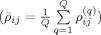
The values of Q and T depend on the problem. For evaluation of single subject analysis, T = 1, and for evaluation of group analysis methods, the number of training datasets is usually set large enough to produce a robust estimate of the activation map. Using a large number of validation datasets (Q) decreases the MI estimation variance but increases the computational cost. We used a leave‐one out crossvalidation approach, where for each of M splits we chose a new one of the M subjects for validation and used the other T = (M − 1) subjects for training. The diagram of the computational steps for evaluation of the MI metric for two datasets is shown in Figure 2 with pseudo‐code outlining the calculation steps in the Appendix.

Figure 2.

A block diagram of the computational steps for evaluation of the MI performance metric. Available independent datasets of an fMRI experiment (y ⁽¹⁾,…,y ^(M)) are preprocessed and then split into two crossvalidation groups for training and validation. Using the training datasets a SPM, s^t, or a label map, c^t, is estimated. The MI between this estimated map and the validation datasets' time‐series is then calculated as an evaluation metric for the analysis technique applied to the training set. The fixed parameters d _y and d _x are distance metrics, respectively, between the validation datasets' high‐dimensional time‐series and the lower dimensional SPM/label map spaces, that allow the MI to be calculated. They are used together with a value of k in a k‐nearest‐neighbor‐based estimate of the MI (see text).

To evaluate the performance of the proposed metric, we compare it with two common measures, asymmetric‐split reproducibility (r) and the JC. The asymmetric‐split reproducibility is defined as the correlation coefficient between the SPMs calculated using T training datasets and the average of the first‐level SPMs of Q ≪ T validation datasets. This measure is similar to the reproducibility metric proposed by Strother et al. [ 1997, 2002] and ICC_WITHIN used by Raemaekers et al. [ 2007] using split‐half resampling (i.e., T = Q). Our proposed MI metric represents a more general measure between spatial maps and time‐series that can be applied to a general crossvalidation data split, with T ≫ Q. How such asymmetric splits relate to split‐half measures (e.g., as used in NPAIRS) and other possible crossvalidation splits is an important one that we are currently investigating.

We use JC to measure the reliability of binary maps calculated by thresholding the two SPMs acquired from T training datasets and from the average of the first‐level SPMs of Q validation datasets. The threshold is chosen such that the relative number of detected active voxels to the total number of intracerebral voxels is γ. JC is the relative number of voxels declared active in both binary maps to the number of voxels detected in at least one binary map. Below, we compare the MI and JC metrics using the same γ.

Simulated fMRI Data

Thirty pairs of simulated fMRI datasets were constructed to evaluate the MI measure and compare its results with those of ROC curves. For each pair, one is used as the training and the other as the validation dataset. The time‐series of the simulated datasets have 128 time points and represent the intensities of a volume with 64 × 64 × 20 voxels versus time. Each time‐series is contaminated with Gaussian noise with the first‐order autoregressive [AR(1)] correlation structure, generated as white Gaussian noise with σ² = 10 filtered by an AR filter with a randomly chosen pole (a) between [0.1, 0.9]. In addition, white Gaussian noise with a variance of 1 was added to the time‐series of each voxel.

The task follows a block design that includes eight blocks, and each block consists of eight active states to eight rest states and the activation level varies between 0.5 and 2 for a maximum possible signal‐to‐noise ratio of about 0.6. The presumed hemodynamic response [Knuth et al., 2001] is given by

(6)

where τ ∈ [0.05,0.21] and σ ∈ [3,7] are randomly chosen for each active voxel [Hossein‐Zadeh et al., 2003a]. The presumed hemodynamic response is convolved with the block‐design box‐car function and then added to the time‐series to create the active voxels with TR = 3. The total number of intracerebral voxels is ∼20,480 of which 1,400 voxels are active voxels, all with amplitudes (activation levels) greater than 0.5.

Real fMRI Data

Data were from an experiment designed to examine cognitive function across several domains [Grady et al., in press]. The stimuli were band‐pass‐filtered visual white noise patches with different center frequencies. During the scans, there were blocks of five conditions: (1) fixation (FIX); (2) simple reaction time to stimulus detection (RT); (3) perceptual matching (PMT); (4) attentional cueing (ATT); and (5) memory (delayed match‐to‐sample, DMS). Four runs were acquired for each subject using a block design with eight alternating task‐fixation conditions (FIX) per run (20 scans/task‐period alternating with 10 scans/fixation‐period, TR = 2 s). Each task occurred twice in each run. We have used one, PMT, to demonstrate the initial utility of the MI metric and then used all four tasks to compare general linear model (GLM) analysis methods. In the RT task, a single stimulus appeared for 1,000 ms in one of three locations at the bottom of the display (left, central, or right), and participants pressed one of three buttons to indicate the location where the stimulus appeared. There were 12 trials in each RT block. In PMT, a sample stimulus appeared centrally in the upper portion of the screen along with three choice stimuli located in the lower part of the screen (for 4,000 ms). The task was to indicate which of the three choice stimuli matched the sample. Six such trials occurred in each PMT block. The ATT task consisted of a sample stimulus appearing for 1,500 ms at the center of the upper part of the screen. After an ISI of 500 ms, an arrow pointing either to the right or to the left was presented for 1,500 ms in the lower part of the screen. After another 500‐ms interval, two stimuli appeared in the right and left locations for 3,000 ms. The task was to attend only to the cued location and press one of two buttons to indicate whether or not the cued target stimulus matched the sample. There were four trials in each ATT block. Finally, in the DMS task, a sample stimulus was presented for 1,500 ms at the center of the upper portion of the screen followed by a delay of 2,500 ms (blank screen). Then, three choice stimuli were presented for 3,000 ms in the lower portion of the screen and the participants had to press one of three buttons to indicate which of the three stimuli matched the previously seen sample. There were four trials in each DMS block. In all tasks, the intertrial interval was 2,000 ms. We report results using the data from the 19 young subjects (21–30 years) that were studied.

Images were acquired with a Siemens Trio 3T magnet. A T1‐weighted anatomical volume using SPGR (TE = 2.6 ms, TR = 2,000 ms, FOV = 256 mm, slice thickness = 1 mm) was also acquired for coregistration with the functional images. T2* functional images (TE = 30 ms, TR = 2,000 ms, flip angle = 70°, FOV = 200 mm) were obtained using EPI acquisition. Each functional sequence consisted of 28 5‐mm‐thick axial slices, positioned to image the whole brain.

Preprocessing

We created an unbiased, nonlinear average anatomical image [Kovacevic et al., 2005], the Common Template. Functional data was slice‐time‐corrected using AFNI (http://afni.nimh.nih.gov/afni) and motion‐corrected using AIR [http://bishopw.loni.ucla.edu/AIR5/; Woods et al., 1998]. For each run, the mean functional volume after motion correction was registered with each subject's structural volume using a rigid body transformation. Transform concatenations were performed: from the initial volume to the reference volume within each run, from the mean‐run volume to the structural volume, and from the structural into the Common Template space. These concatenated transforms were applied to register the data using a direct nonlinear transform from each initial fMRI volume into the Common Template space with a voxel size of 4 mm³. Finally, spatial smoothing was performed on the registered data using a 3‐D spatial Gaussian filter with full width half maximum (FWHM) = 7 mm.

RESULTS

Simulation Data

To evaluate our proposed method and its consistency with ROC curves, we used the thirty training simulation datasets to compare different processing approaches. We derived the average ROC curves over thirty simulated training datasets for canonical correlation analysis [CCA; Friman et al., 2001] with a 3 × 3 neighborhood, the GLM with a white Gaussian noise model [Friston et al., 1995], GLM with an autoregressive noise model [GLM‐AR; Bullmore et al., 2001], CVA [Neilsen et al., 1998; Strother et al., 1997], a time‐invariant wavelet transform (TIWT) method using Daubechies wavelet with four vanishing moments [Hossein‐Zadeh et al., 2003b]. The CVA used a singular value decomposition (SVD) to reduce the simulated data dimension by calculating the CVA on the first 10 SVD components. Since we did not intend to compare optimized versions of the abovementioned methods, we did not tune their parameters for their best performance.

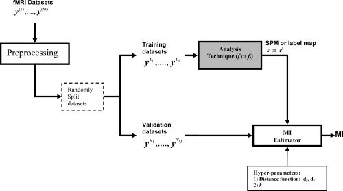
For each statistical method, the relative number of truly detected voxels (probability of detection) and falsely detected voxels (false alarms) are calculated after thresholding their SPMs. The plot of estimated probability of true‐positive detections versus false‐positive alarms for different thresholds provides empirical ROC curves for each analysis technique. The average ROC curves over thirty training datasets for the five statistical analysis methods are shown in Figure 3a. For this simulation, none of the models perform particularly well with a maximum detection rate of 0.4 achieved by the two multivariate techniques for a false‐alarm rate of 0.1. The partial areas under the ROC curves (ROC_PA) for false alarms between 0 and 0.1 were calculated for each of the five analysis techniques on the thirty simulated training datasets.

Figure 3.

(a) The average ROC curves for different analysis methods applied to the simulated datasets. The methods are CCA, CVA, GLM‐AR, GLM with a white Gaussian noise model, and TIWT. The partial areas under ROC curves (0 < false alarm < 0.1) of CCA, CVA, GLM‐AR, GLM, and TIWT are 0.0525, 0.0386, 0.0325, 0.0318, and 0.0312, respectively. (b) Mean ranks of CCA, CVA, GLM‐AR, GLM, and TIWT measured by the partial area under ROC curve for 0 < false alarm < 0.1 over 30 simulated datasets. A CD diagram based on a nonparametric Friedman difference test by ranks is shown in the right panel. The CD range (α = 0.05) for significant rank differences allowing for multiple comparisons is marked next to the best‐performing technique with rank = 1, i.e., CCA.

We used a nonparametric Friedman test to explore whether there are significant differences between the ROC_PA values across analysis techniques [Friedman test; treatment = single‐subject analysis techniques, samples = the partial area under the ROC curves; Conover, 1999]. The test shows that different methods result in significantly different ROC_PA (p < 0.001). As the null‐hypothesis of no analysis technique differences is rejected, we proceed with the Nemenyi test [Demsar, 2006; Nemenyi, 1963] to pairwise compare the methods to each other. The ROC_PA of two methods is significantly different if the corresponding average ranks differ by at least a critical difference [CD; Demsar, 2006; Nemenyi, 1963)]. The mean rank of each analysis technique is shown in Figure 3b. Rank 1 corresponds to the largest ROC_PA. The CD for α = 0.05 is shown to the right of rank 1, and all the analysis techniques have significantly different performance with average ranks greater than the CD apart.

For each of the five single‐subject analysis techniques, we calculated 30 values of MI from the 30 pairs of training and validation simulated datasets. In Figure 4, the MI with k = 20 (see below) is estimated based on the MI method for binary labeled data [i.e., g(f(y ^t))] as a function of a range of SPM thresholds (γ) and for the continuous MI metric. In Figure 4a, the median of MI_BINARY is plotted versus γ in the simulated datasets. The plots rank models identically to the ROC curves for false alarms less than ∼0.05 (see Fig. 3). Both multivariate methods, CCA and CVA, have better MI values than the univariate techniques for γ < 0.3, and their MI_BINARY curves peak near γ = 0.075, close to the actual ratio of active voxels in the simulated datasets (1,400/20,480 = 0.068). The MI_CONTINUOUS values of each processing method are shown in Figure 4b and are rank ordered identically to the ROC results (see Fig. 3), and the MI_BINARY results in Figure 4a. This shows that MI is consistent with ROC curves for both label maps and continuous maps for k = 20.

Figure 4.

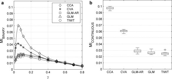
(a) The median of MI_BINARY calculated for and plotted against the fraction of positive SPM values, γ, for different single‐subject analysis techniques (see Fig. 3) applied to the simulated datasets. (b) MI_CONTINUOUS for different single‐subject techniques (see Fig. 3) applied to the simulated datasets. The rankings of the analysis techniques acquired by MI_BINARY and MI_CONTINUOUS and shown above are consistent with their true rankings acquired by ROC curves as shown in Figure 3 (for statistical tests of analysis rankings, see Fig. 5).

Figure 5a shows the mean rank of each analysis technique acquired using MI_CONTINUOUS for k = 1, 20, 100, 500. The null‐hypothesis of no significant difference between the techniques is rejected in each case (p < 0.001), and so we proceeded with pairwise comparisons of the five single‐subject analysis techniques. Rank 1 corresponds to the largest MI value, and the CD for α = 0.05 is shown as a black line above the Rank 1 result. For k = 1, MI_CONTINUOUS cannot detect any significant difference between CCA and CVA or between GLM‐AR, GLM, and TIWT (CD = 1.36). Using k = 20, MI_CONTINUOUS detects significant differences between all five analysis techniques (CD = 0.42). For k = 1, 20, and 100, the average rankings of the analysis techniques are consistent with the ROC curves, but for k = 100 MI_CONTINUOUS cannot differentiate between GLM‐AR and GLM (CD = 0.78). For k = 500, which includes more than 1/3 of the total number of active voxels, the rankings are not consistent with the ROC curves, and many pairwise comparisons are not significantly different. The minimum CD occurs for k = 20, showing that MI_CONTINUOUS has maximum sensitivity around k ≈ 20 in this simulated dataset.

Figure 5.

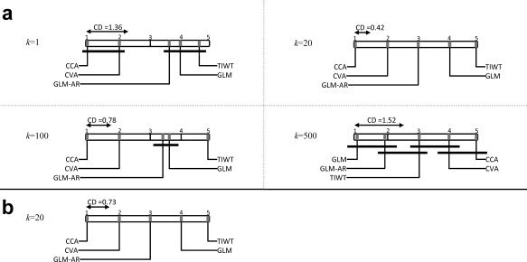
CD diagrams of mean rankings based on a nonparametric Friedman difference test by ranks for analysis of the simulated dataset with (a) CCA, CVA, GLM‐AR, GLM and TIWT measured by MI_CONTINOUS for neighborhood values of k = 1, 20, 100, and 500 (see Fig. 2) and (b) CCA, CVA, GLM‐AR, GLM, and TIWT measured by MI_BINARY (γ = 0.1) for k = 20. The CD range within which ranks are not significantly different (α = 0.05) allowing for multiple comparisons is illustrated as a line segment starting at Rank 1 above each diagram. Rank 1 corresponds to the best‐performing analysis with the highest average MI measurement. MI metrics for (a) k = 1, 20, 100 and (b) k = 20 are consistent with the partial area under the ROC curves (see Fig. 3). All analysis techniques are ranked as significantly different only for k = 20 with MI_CONTINOUS and MI_BINARY.

These results in Figure 5a illustrate the bias‐variance trade‐off in estimation of the MI_CONTINUOUS metric. If we assume that the time‐series of each active voxel is similar to that of a small number of neighborhood voxels and choose a small value for the neighborhood size (k), we will have high variance in estimation of the metric but the bias of estimation will be relatively low. This means that the ranking of the methods will be consistent with the true rankings on average, but the MI metric may be too noisy to significantly differentiate between similar methods (see Fig. 5a for k = 1). For large neighborhood sizes, the variance of the MI metric will be low but with a high bias in ranking of the analysis techniques producing average rankings that may not be consistent with the true performance represented by the ROC curves (see Fig. 5a for k = 500).

In Figure 5b, the mean rank of each analysis technique acquired using MI_BINARY (γ = 0.1) for k = 20 is shown. MI_BINARY ranks techniques identically to the ROC results (see Fig. 3) and detects that all five analysis techniques are significantly different. As we get reasonable sensitivity for k = 20 in our simulation datasets, we have used the same k for real fMRI data in this article. Ideally k should be optimized in a validation resampling step and then MI tested for that value of k using independent test data. However, this is not currently computationally feasible in our laboratory with typical real fMRI datasets.

To show the difference between the modified MI estimator and the original MI estimation proposed by Kraskov et al. [ 2004], we use their MI estimation code (available at http://www.klab.caltech.edu/~kraskov/MILCA/) without any dimension reduction and apply it to the simulated datasets (k = 20). As above, we use a nonparametric Friedman test to test whether the MI metric from Kraskov can detect any significant difference between the five analysis techniques. The omnibus test is not rejected (p = 0.36) indicating that MI estimation in such a high‐dimensional space with Kraskov's max norm has a large variance.

Real fMRI Data

We used the software packages SPM5 [http://www.fil.ion.ucl.ac.uk/spm/; Friston et al., 2007] and FSL4.0 [http://www.fmrib.ox.ac.uk/fsl/; Smith et al., 2004] to analyze the datasets. The software packages SPM5 and FSL4.0 are GLM‐based methods that use different methods for estimation of the noise covariance matrix and calculation of the effective degrees of freedom used for statistical inference in the first‐level analysis. In the second level, SPM5 is an OLS estimator when only one task contrast at a time is used, which is the case in this article. The OLS estimator in FSL4.0 was used to run the second‐level analysis (FSL‐OLS).

The design matrix for GLM‐based methods (SPM5, FSL4.0) includes a hemodynamic response modeled by two gamma functions and their derivatives. The gamma functions implemented inside each software package with their default settings for the parameters are used. We used the implemented high‐pass filters in the respective SPM5 and FSL packages with a cut‐off frequency of 0.01 Hz to remove low‐frequency fluctuations, trends, and voxel time‐series means. Performance differences between FSL‐OLS and SPM5 could result from differences in noise parameter estimation, high‐pass filtering, hemodynamic response model, etc. We used the MI metric to deliberately compare the whole processing pipeline in SPM5 and FSL‐OLS with their default settings. We believe the comparison of default settings is useful for the field because it represents a common mode of operation for many papers produced with the two packages under the assumption that the developers have chosen semioptimal default parameter settings.

We randomly split the datasets 16 times into training sets with 10 or 15 subjects and validation sets with 1 subject, producing 16 estimated MI values for each of the two training set sizes. The validation subject for 10 and 15 training subjects is the same for each split but different between splits. In addition, the same splits are used to acquire Jaccard and reproducibility metrics. This allows us to perform a pairwise Student's t‐test and compare the sensitivity of the MI, reproducibility, and Jaccard metrics. The detected active areas (|z| > 1.96) in two slices of PMT contrasts using FSL‐OLS and SPM5 for 10 and 15 training subjects are shown in Figure 6.

Figure 6.

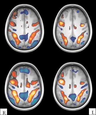
Positively and negatively thresholded voxels (|z| > 1.96) for the perceptual matching task versus fixation analyzed with FSL‐OLS (left column) and SPM5 (right column) of 10 subjects (the first row) and 15 subjects (the second row).

We estimated the MI_CONTINUOUS and MI_BINARY for FSL‐OLS and SPM5 applied to the 10 and 15 training subjects for PMT versus Fixation contrasts. Note that the same preprocessing steps such as motion correction, smoothing, and high‐pass filtering are performed on both the training and validation datasets. The MI metrics were estimated using those segments of validation time‐series where the subjects were performing the PMT and adjacent Fixation tasks to remove the effects of other tasks.

The SPMs acquired using 15 compared to 10 subjects are expected to have more power and higher MI metrics. We used this to test the effect of the number of subjects in the training set (T) on the MI metrics (MI_CONTINUOUS and MI_BINARY), asymmetric‐split reproducibility (r), and JC. The metric that is most sensitive to increasing the group size may be rated as a better metric. Figure 7 shows the performance of FSL‐OLS and SPM5 for T = 10 and T = 15 measured with MI_CONTINUOUS, asymmetric‐split reproducibility (r), MI_BINARY, and JC. For all four metrics and their plots (Fig. 7a–d), the medians of the box–whisker distributions are seen to rise with increasing numbers of subjects showing that increasing the group size increases the performance of the analysis techniques.

Figure 7.

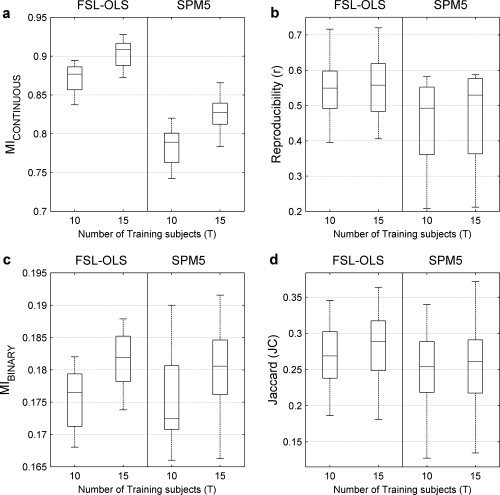
Results from analysis of the perceptual matching task versus fixation analyzed with FSL‐OLS (left column) and SPM5 (right column) in each panel for training groups of T = 10 and T = 15 young subjects: (a) MI_CONTINUOUS; (b) asymmetric‐reproducibility (r) (see text); (c) MI_BINARY for the fraction of positive SPM values, γ = 0.1; (d) the Jaccard metric (JC). The line in the middle of each box–whisker plot is the sample median. All measures use the same leave‐one‐out crossvalidation scheme (see text). MI_CONTINUOUS and MI_BINARY are more sensitive than asymmetric reproducibility and the Jaccard metric in differentiating between T = 10 and T = 15.

Comparing Figure 7a and Figure 7b, the nonoverlapping distributions of the MI_CONTINUOUS measure are seen to be more sensitive to differences between methods and the group size than the largely overlapping distributions of the asymmetric‐split reproducibility correlation coefficients. In Figure 7c,d, for each model with γ = 0.1, the MI_BINARY metric distributions have somewhat less overlap and more separated medians than the Jaccard metric distributions with increasing group size. In addition, when comparing MI_CONTINUOUS in Figure 7a with MI_BINARY in Figure 7c, we see that for the same analysis technique thresholding with γ = 0.1 loses information. Furthermore, both MI metrics and to some extent the asymmetric‐split reproducibility values reflect a tendency for FSL‐OLS to more efficiently extract information from the data for a given percentile activation threshold.

To quantitatively evaluate these apparent sensitivity differences, we used a pairwise Student's t‐test to test for significant metric differences between the training groups of T = 10 and T = 15 subjects. Table I reports the pairwise t‐test statistics, which are calculated separately for FSL‐OLS and SPM5. Based on the magnitude of the estimated t‐tests, there is evidence that the MI_CONTINUOUS measures are significantly more sensitive than the asymmetric reproducibility and Jaccard measures. The MI_BINARY (γ = 0.1) is somewhat more sensitive than Reproducibility and Jaccard for FSL‐OLS, but it is less sensitive for SPM5.

Table I.

t Statistics and significance levels for different MI metrics, asymmetric reproducibility (r), and the Jaccard metric (JC)

	MICONTINUOUS	MIBINARY (γ = 0.1)	Reproducibility (r)	Jaccard (γ = 0.1)
FSL‐OLS	15.37**	4.53**	3.38*	3.03*
SPM5	12.02**	2.56	3.32*	3.95**

For subjects performing the perceptual matching task and SPMs from FSL‐OLS and SPM5, a pairwise Student's t‐test is used to determine the significance of the difference between the Training groups of subjects for T = 10 and T = 15 (see Fig, 7).

^* p < 0.05 corrected for multiple comparisons;

^** p < 0.01 corrected for multiple comparisons.

In Figure 8a, the MI_BINARY measured from FSL‐OLS and SPM5 for 10 and 15 training subjects is shown versus γ. In Figure 8b, MI_BINARY for 0.05 < γ < 0.125 is shown. SPM5 outperforms FSL‐OLS for γ < 0.1 for both T = 10 and T = 15, but FSL‐OLS has a superior performance with higher γs. Therefore, depending on the fraction of activated voxels identified by a particular false discovery rate (FDR; see Table II), detection performance may be more dependent on the choice of GLM model than a 50% increase in the number of subjects. In Table II, we report the relative number of detected voxels (γ) and MI_BINARY for FSL‐OLS and SPM5, for T = 10 and T = 15 and for three values of FDR, 0.005, 0.01 and 0.05. With FDR = 0.005, FSL‐OLS for T = 10 identifies the same fraction of active voxels (γ = 0.1) as SPM5 with T = 15. For an increasing fraction of nominally active voxels, MI and FDR are related for all models and training set sizes, and at a fixed FDR, GLM using FSL‐OLS extracts more voxels and more information (i.e., MI_BINARY) than SPM5 in both group sizes. Furthermore, at a fixed FDR, the increased fraction of activated voxels for T = 15 versus T = 10 is associated with greater information extraction for T = 15 with either GLM technique as expected.

Figure 8.

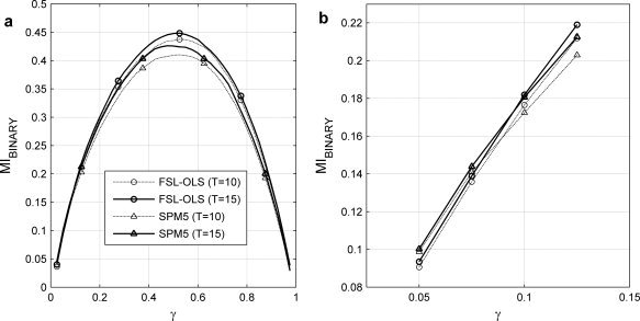
MI_BINARY results from analysis of the perceptual matching task versus fixation analyzed with FSL‐OLS and SPM5 for training set groups of T = 10 and T = 15 subjects as a function of (a) the fraction of SPM values, γ from 0.0 to 1.0, and (b) for 0.05 < γ < 0.125. SPM5 performs better than FSL‐OLS for γ ≤ 0.1 in both group sizes, but FSL‐OLS has better performance with higher γs.

Table II.

The fraction of all voxels declared active (γ) and MI_BINARY for different FDR levels using FSL‐OLS and SPM5 applied to training groups of 10 and 15 young subjects

	Analysis technique	FDR
		0.005	0.01	0.05
T = 10	FSL‐OLS
	γ	0.10	0.13	0.23
	MIBINARY	0.22	0.26	0.37
	SPM5
	γ	0.06	0.08	0.13
	MIBINARY	0.16	0.18	0.25
T = 15	FSL‐OLS
	γ	0.20	0.23	0.31
	MIBINARY	0.34	0.37	0.43
	SPM5
	γ	0.10	0.12	0.19
	MIBINARY	0.22	0.24	0.33

In real datasets, the peaks of the MI_BINARY curves are near γ = 0.5, indicating that the most separable clusters in time‐series space are created for γ ≈ 0.5. This optimal threshold fraction is very different from the simulated dataset where the multivariate peaks are around 0.075 with univariate peak thresholds closer to 0.1. This difference between real and simulated datasets may be due to the simulated data having only positive BOLD changes (Task mode). In the real fMRI datasets, there are both strong positive and negative (Default mode) BOLD changes that create two strong clusters in time‐series space. Also, in the real datasets, the separation of the time‐series into different clusters has been increased by applying spatial smoothing. Finally, the MI metrics for real datasets are much larger than MI metrics for simulated datasets. This demonstrates that real datasets are more information‐rich than simple simulated datasets such as those used here.

Figure 9 shows the performance of FSL‐OLS and SPM5 for all four tasks (ATT, DMS, PMT, and RT) versus Fixation measured by MI_CONTINUOUS. To calculate the MI metric for a specific task, we used those segments of validation subjects' time‐series when the subjects were performing the task or in the Fixation state. This removes the effects of the other tasks in evaluation of an analysis technique for a specific task contrast. As shown in Figure 9, FSL‐OLS with its default settings performs better than SPM5 with its default settings for all task contrasts. However, we did not tune the parameters inside each software package for their best performance, and for other setting of the parameters, their relative performance might change.

Figure 9.

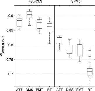
The performance of FSL‐OLS and SPM5 measured by MI_CONTINUOUS. FSL‐OLS performs better than SPM5 for all task contrasts.

DISCUSSION

This article introduces an evaluation method based on MI to assess fMRI analysis techniques without knowing the ground truth. To our knowledge, this is the first technique for measuring analysis performance in fMRI that compares SPMs from any model against independent time‐series, without requiring any of the modeling assumptions that generated the SPM. This is an extension of standard prediction and reproducibility metrics, which use the same modeling framework and assumptions to both generate a reliable SPM and predict a related label structure in an independent time‐series (e.g., the NPAIRS framework). We have shown that these MI metrics may be significantly more sensitive than other modeling performance measures such as asymmetric‐split reproducibility and the Jaccard (or DICE) overlap statistic.

In addition, MI also provides a new measure of information extraction that may be used to identify nominally activated voxels for comparison with thresholding procedures such as FDR. Furthermore, removing the need to know a label structure in the independent, validation time‐series opens up a broad class of experiments. With the MI metrics a SPM can be generated using any analysis model in one experiment and then tested for its relative expression, on an MI scale, in time‐series from arbitrary related or unrelated experiments, e.g., to rank activation pattern and network expression across different tasks.

To calculate the MI between a spatial SPM and independent time‐series from the same or different experiments, we used a method based on k‐nearest neighbors. This method appears to perform well even when only weak signals exist, such as in simulations with only a small number of active voxels or in relatively small groups of subjects. The parameter k and the SPM‐ and time‐series distance measures used to estimate MI are parameters that allow SPMs to be linked to arbitrary, independent time‐series: (1) for MI_BINARY by determining the form of the separating boundary between two time‐series clusters of active and non‐active voxels defined by the thresholded SPM or (2) for MI_CONTINUOUS by comparing the interval ranking of the distance between voxel pairs in the SPM to the distance between the corresponding voxel pairs in the time‐series.

MI metrics share the advantage with NPAIRS prediction and reproducibility metrics of depending on both generalizable spatial and temporal consistency evaluated in a crossvalidation framework, which distinguishes them from other performance metrics as outlined in the Introduction. Such approaches go some way to ensuring better generalization of fMRI results and can provide evidence of the generalization through replication needed to develop “strong inferences” [Platt, 1964] and avoid circular analysis [Kriegeskorte et al., 2009].

However, there are still some fMRI artifacts that may be spatially reproducible with somewhat consistent temporal structure in different repetitions of an fMRI experiment, particularly in single‐subject analysis [e.g., Fig. 1, Chen et al., 2006]. Such spatially reproducible artifacts may create spurious clusters in time‐series space and cause an error in ranking the methods, even in a spatiotemporal crossvalidation framework. Therefore, when comparing analysis techniques, it is important that careful attention is paid to removal of such artifacts (e.g., some motion‐related effects, other low‐frequency temporal trends, potential white‐matter bias, etc.) from both training and validation datasets using similar preprocessing pipelines.

Our results show that the MI metric for binary maps is always smaller than the MI metric for continuous maps. This confirms the fact that information is lost via thresholding procedures, which are removing more than simple random noise voxels. This loss is clearly seen in the simulated datasets where MI_BINARY < MI_CONTINUOUS, but both metrics rank the analysis techniques in the same order as ROC curves. Furthermore, MI metrics for simulated datasets and MI_BINARY < MI_CONTINUOUS differences (see Fig. 4) are much smaller than those seen in real fMRI datasets (Figs. 7 and 8). These results show that our simple simulated dataset does not capture the structure of real fMRI datasets, and therefore comparing analysis techniques using such simulations is likely to be biased. This is one of the primary motivations for developing data‐driven performance metrics such as MI. Furthermore, the two MI metrics could be used to test the similarity of any particular simulation to any real dataset.

We also used the MI‐based metrics to compare the implemented OLS methods in SPM5 and FSL together with their respective high‐pass filtering approaches and other default parameter settings. These GLM‐based software packages use different models for temporal noise whitening of fMRI time‐series and different temporal filtering approaches; as a result, they create different SPMs from the same data. In our data, based particularly on measures of MI_CONTINUOUS (Figs. 7a and 9) and MI_BINARY at a fixed FDR, there is strong evidence that the FSL processes may significantly outperform those of SPM5. However, based on MI_BINARY (Fig. 8b), the SPM5 processes may outperform FSL for peak, active voxel fractions that are approximately defined by γ < 0.1 and underperform against FSL processes for γ > 0.1. We are currently testing both of these preliminary results across multiple datasets as a function of age and extending them to include a comparison with NPAIRS metrics and associated multivariate analysis techniques. Overall, these results and the relationship between FDR and MI_BINARY seen in Table II suggest that FDR and related absolute statistical thresholds based on controlling Type 1 errors may be poor approaches to understanding the information content of SPMs and information extraction with thresholding.

CONCLUSION

In this article, we have introduced a powerful new measure based on the MI between spatial activation patterns and independent fMRI time‐series for evaluating the performance of fMRI data analysis techniques without ground truth. This technique generalizes the use of a single modeling framework, which underlies the temporal prediction and spatial reproducibility metrics within the NPAIRS framework. This allows a SPM from a particular model to be compared with any arbitrary independent time‐series without knowing its experimental design structure (e.g., condition labels). We show that our MI metric is consistent with ROC measures in simulations and more sensitive than reproducibility or Jaccard metrics for detecting improved activation maps in real datasets.

The Shannon entropy of a continuous random variable (or vector) x measures the amount of uncertainty or lack of information in that variable and is defined as , where P(x) is the probability density function of x. The MI between two random variables (or vectors) x and y defined in Eq. (2) may be expressed in terms of Shannon entropy as follows [Cover and Thomas, 1991]:

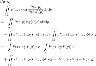(A1)

The same relation between the MI and Shannon entropy exists when x is a binary random variable. In Kraskov et al. [ 2004], the Shannon entropy terms in Eq. (A1) is estimated based on a k‐nearest neighbor based algorithm as follows:

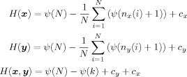(A2)

where c _x and c _y are two terms that depend on the observation x _i and y _i for i = 1, …, N. n _x(i), n _y(i), and ψ(.) are defined in “Estimating the MI Metric” subsection. By substituting the estimated entropy of x and y, and the joint entropy (x,y) from Eq. (A2) into Eq. (A1) the terms c _x and c _y are canceled out and the estimation of MI based on a k‐nearest neighbor approximation as defined in Eq. (6) is obtained.

The pseudocode for our modified k‐nearest neighbor‐based MI algorithm is as follows (see Fig. 1):

• 1 I ← ψ(k) + ψ(N)
• 2
  For i = 1 to N

  • a
    Calculate the distance between the voxel i and the remaining N − 1 voxels in SPM space
  • b
    Calculate the distance between the voxel i and the remaining N − 1 voxels in time‐series space
  • c
    Calculate the distance between the voxel i and the remaining N − 1 voxels in the joint space
  • d
    Sort the N − 1 voxels from the nearest to the farthest based on their distance in joint space
  • e
    Find the kth nearest voxel from the ranked list in (d). Its distance in joint space defines the neighborhood size (ε_z(i)).
  • f
    Count the number of voxels j such that d _x(x _i, x _j) ≤ ε_z(i) (n _x(i))
  • g
    Count the number of voxels j such that d _y(y _i, y _j) ≤ ε_z(i) (n _y(i)).
  • h
    I ← I − (ψ(n _x(i) + 1) + ψ(n _y(i) + 1))/N
• 3End for

REFERENCES

- Blinnikov S, Moessner R ( 1998): Expansions for nearly Gaussian distributions. Astron Astrophys Suppl Ser 130: 193–205. [Google Scholar]
- Borg I, Groenen PJF ( 2005): Modern Multidimensional Scaling: Theory and Applications. London: Springer; xxi, 614 p. [Google Scholar]
- Bouix S, Martin‐Fernandez M, Ungar L, Nakamura M, Koo M‐S, McCarley RW, Shenton ME ( 2007): On evaluating brain tissue classifiers without a ground truth. Neuroimage 36: 1207–1224. [DOI] [PMC free article] [PubMed] [Google Scholar]
- Bullmore E, Long C, Suckling J, Fadili J, Calvert G, Zelaya F, Carpenter T, Brammer M ( 2001): Colored noise and computational inference in neurophysiological (fMRI) time series analysis: Resampling methods in time and wavelet domains. Hum Brain Mapp 12: 61–68. [DOI] [PMC free article] [PubMed] [Google Scholar]
- Cellucci CJ, Albano AM, Rapp PE ( 2005): Statistical validation of mutual information calculations: Comparison of alternative numerical algorithms. Phys Rev E 71: 066208. [DOI] [PubMed] [Google Scholar]
- Chen EE, Small SL ( 2007): Test–retest reliability in fMRI of language: Group and task effects. Brain Lang 102: 176–185. [DOI] [PMC free article] [PubMed] [Google Scholar]
- Chen X, Pereira F, Lee W, Strother S, Mitchell T ( 2006): Exploring predictive and reproducible modeling with the single‐subject FIAC dataset. Hum Brain Mapp 27: 452–461. [DOI] [PMC free article] [PubMed] [Google Scholar]
- Cohen J ( 1960): A coefficient of agreement for nominal scales. Educ Psychol Meas 20: 37–46. [Google Scholar]
- Colwell RK, Coddington JA ( 1994): Estimating terrestrial biodiversity through extrapolation. Philos Trans R Soc Lond B Biol Sci 345: 101–118. [DOI] [PubMed] [Google Scholar]
- Conover WJ ( 1999): Practical Nonparametric Statistics. New York: Wiley; pp 269–427. [Google Scholar]
- Cover TM, Thomas JA ( 1991): Elements of Information Theory. New York: Wiley; p 32. [Google Scholar]
- Cox TF, Cox MAA ( 1994): Multidimensional Scaling. London: Chapman & Hall; x, 213 p. [Google Scholar]
- Darbellay GA, Vajda I ( 1999): Estimation of the information by an adaptive partitioning of the observation. IEEE Trans Inf Theory 45: 1315–1321. [Google Scholar]
- Daub CO, Steuer R, Selbig J, Kloska S ( 2004): Estimating mutual information using B‐spline functions—An improved similarity measure for analysing gene expression data. BMC Bioinformatics 5: 118. [DOI] [PMC free article] [PubMed] [Google Scholar]
- Davis PJ ( 1972): Gamma function and related functions In: Abramowitz M, Stegun IA, editors. Handbook of Mathematical Functions: With Formulas, Graphs, and Mathematical Tables. New York: Dover; pp 258–259. [Google Scholar]
- Demsar J ( 2006): Statistical comparisons of classifiers over multiple data sets. J Mach Lear Res 7: 1–30. [Google Scholar]
- Dice LR ( 1945): Measures of the amount of ecologic association between species. Ecology 26: 297–302. [Google Scholar]
- Frackowiak RSJ, Ashburner JT, Penny WD, Zeki S ( 2004): Spatial normalization using basis functions In: Friston KJ, Frith CD, Dolan RJ, Price CJ, editors. Human Brain Function, 2nd ed. San Diego, CA: Academic Press; pp 655–672. [Google Scholar]
- Friedman L, Stern H, Brown GG, Mathalon DH, Turner J, Glover GH, Gollub RL, Lauriello J, Lim KO, Cannon T, Greve DN, Bockholt HJ, Belger A, Mueller B, Doty MJ, He J, Wells W, Smyth P, Pieper S, Kim S, Kubicki M, Vangel M, Potkin SG ( 2008): Test–retest and between‐site reliability in a multicenter fMRI study. Hum Brain Mapp 29: 958–972. [DOI] [PMC free article] [PubMed] [Google Scholar]
- Friman O, Cedefamn J, Lundberg P, Borga M, Knutsson H ( 2001): Detection of neural activity in fMRI using canonical correlation analysis. Magn Reson Med 45: 323–330. [DOI] [PubMed] [Google Scholar]
- Friston K, Holmes A, Worsley K, Poline J‐P, Frith C, Frackowiak R ( 1995): Statistical parametric maps in functional neuroimaging: A general linear approach. Hum Brain Mapp 2: 189–210. [Google Scholar]
- Friston KJ, Ashburner JT, Kiebel S, Nichols TE, Penny WD, editors ( 2007): Statistical Parametric Mapping: The Analysis of Functional Brain Images, 1st ed. Boston: Academic Press; pp 101–211. [Google Scholar]
- Genovese CR, Noll DC, Eddy WF ( 1997): Estimating test–retest reliability in functional MR imaging I: Statistical methodology. Magn Reson Med 38: 497–507. [DOI] [PubMed] [Google Scholar]
- Golay X, Kollias S, Stoll G, Meier D, Valavanis A, Boesiger P ( 1998): A new correlation‐based fuzzy logic clustering algorithm for FMRI. Magn Reson Med 40: 249–260. [DOI] [PubMed] [Google Scholar]
- Gomez‐Laberge C, Adler A, Cameron I, Nguyen TT, Hogan MMJ ( 2008): Selection criteria for the analysis of data‐driven clusters in cerebral fMRI. IEEE Trans Biomed Eng 55: 2372–2380. [DOI] [PubMed] [Google Scholar]
- Grady CL, Protzner A, Kovacevic N, Strother SC, Afshin‐Pour B, Wojtowicz M, Anderson J, Churchill N, McIntosh AR: A multivariate analysis of age‐related differences in the default mode and task positive networks across multiple cognitive domains. Cereb Cortex (in press). [DOI] [PMC free article] [PubMed] [Google Scholar]
- Gullapalli RP, Maitra R, Roys S, Smith G, Alon G, Greenspan J ( 2005): Reliability estimation of grouped functional imaging data using penalized maximum likelihood. Magn Reson Med 53: 1126–1134. [DOI] [PubMed] [Google Scholar]
- Hansen LK, Larsen J, Nielsen FA, Strother SC, Rostrup E, Savoy R, Svarer C, Paulson OB ( 1999): Generalizable patterns in neuroimaging: How many principal components? Neuroimage 9: 534–544. [DOI] [PubMed] [Google Scholar]
- Hossein‐Zadeh GA, Ardekani BA, Soltanian‐Zadeh H ( 2003a): A signal subspace approach for modeling the hemodynamic response function in fMRI. Magn Reson Imaging 21: 835–843. [DOI] [PubMed] [Google Scholar]
- Hossein‐Zadeh GA, Soltanian‐Zadeh H, Ardekani BA ( 2003b): Multiresolution fMRI activation detection using translation invariant wavelet transform and statistical analysis based on resampling. IEEE Trans Med Imaging 22: 302–314. [DOI] [PubMed] [Google Scholar]
- Hripcsak G, Heitjanb DF ( 2002): Measuring agreement in medical informatics reliability studies. J Biomed Inform 35: 99–110. [DOI] [PubMed] [Google Scholar]
- Jaccard P ( 1901): Etude comparative de la distribution florale dans une portion des Alpes et des Jura. Bull Soc Vaudoise Sci Nat 37: 547–579. [Google Scholar]
- Jacobsen DJ, Hansen LK, Madsen KH ( 2008): Bayesian model comparison in nonlinear BOLD fMRI hemodynamics. Neural Comput 20: 738–755. [DOI] [PubMed] [Google Scholar]
- Khan S, Bandyopadhyay S, Ganguly AR, Saigal S, Erickson DJ, Protopopescu V, Ostrouchov G ( 2007): Relative performance of mutual information estimation methods for quantifying the dependence among short and noisy data. Phys Rev E 76: 026209. [DOI] [PubMed] [Google Scholar]
- Kjems U, Hansen LK, Anderson J, Frutiger S, Muley S, Sidtis J, Rottenberg D, Strother SC ( 2002): The quantitative evaluation of functional neuroimaging experiments: Mutual information learning curves. Neuroimage 15: 772–786. [DOI] [PubMed] [Google Scholar]
- Knuth KH, Ardekani BA, Helpern JA ( 2001): Bayesian estimation of a parameterized hemodynamic response function in an event‐related fMRI experiment. Poster presented at the proceedings of International Society for Magnetic Resonance in Medicine (ISMRM) 2001, Ninth Scientific Meeting, Berkeley, CA, No. 1732.
- Kovacevic N, Henderson JT, Chan E, Lifshitz N, Bishop J, Evans AC, Henkelman RM, Chen XJ ( 2005): A three‐dimensional MRI atlas of the mouse brain with estimates of the average and variability. Cereb Cortex 15: 639–645. [DOI] [PubMed] [Google Scholar]
- Kraskov A, Stögbauer H, Grassberger P ( 2004): Estimating mutual information. Phys Rev E 69: 066138. [DOI] [PubMed] [Google Scholar]
- Kriegeskorte N, Simmons WK, Bellgowan PS, Baker CI ( 2009): Circular analysis in systems neuroscience: The dangers of double dipping. Nat Neurosci 12: 535–540. [DOI] [PMC free article] [PubMed] [Google Scholar]
- LaConte S, Anderson J, Muley S, Ashe J, Frutiger S, Rehm K, Hansen LK, Yacoub E, Hu X, Rottenberg D, Strother S ( 2003): The evaluation of preprocessing choices in single‐subject BOLD fMRI using NPAIRS performance metrics. Neuroimage 18: 10–27. [DOI] [PubMed] [Google Scholar]
- LaConte S, Strother S, Cherkassky V, Anderson J, Hu X ( 2005): Support vector machines for temporal classification of block design fMRI data. Neuroimage 26: 317–329. [DOI] [PubMed] [Google Scholar]
- Le TH, Hu X ( 1997): Methods for assessing accuracy and reliability in functional MRI. NMR Biomed 10( 4/5): 160–164. [DOI] [PubMed] [Google Scholar]
- Machielsen WC, Rombouts SA, Barkhof F, Scheltens P, Witter MP ( 2000): fMRI of visual encoding: Reproducibility of activation. Hum Brain Mapp 9: 156–164. [DOI] [PMC free article] [PubMed] [Google Scholar]
- Maitra R ( 2009): Assessing certainty of activation or inactivation in test–retest fMRI studies. Neuroimage 47: 88–97. [DOI] [PubMed] [Google Scholar]
- Maitra R ( 2010): A re‐defined and generalized percent‐overlap‐of‐activation measure for studies of fMRI reproducibility and its use in identifying outlier activation maps. Neuroimage 50: 124–135. [DOI] [PubMed] [Google Scholar]
- Maitra R, Roys SR, Gullapalli RP ( 2002): Test–retest reliability estimation of functional MRI data. Magn Reson Med 48: 62–70. [DOI] [PubMed] [Google Scholar]
- McGonigle DJ, Howseman AM, Athwal BS, Friston KJ, Frackowiak RSJ, Holmes AP ( 2000): Variability in fMRI: An examination of intersession differences. Neuroimage 11: 708–734. [DOI] [PubMed] [Google Scholar]
- Moon Y‐I, Rajagopalan B, Lall U ( 1995): Estimation of mutual information using kernel density estimators. Phys Rev E 52: 2318–2321. [DOI] [PubMed] [Google Scholar]
- Mørch N, Hansen LK, Strother SC, Svarer C, Rottenberg DA, Lautrup B, Savoy R, Paulson OB ( 1997): Nonlinear versus linear models in functional neuroimaging: Learning curves and generalization crossover In: Duncan J, Gindi G, editors. Information Processing in Medical Imaging. New York: Springer; pp 259–270. [Google Scholar]
- Neilsen F, Hansen LK, Strother SC ( 1998): Canonical ridge analysis with ridge parameter optimization. Neuroimage 7: S758. [Google Scholar]
- Nemenyi P ( 1963): Distribution‐free multiple comparisons. Ph.D. thesis, Princeton University.
- Paninski L ( 2003): Estimation of entropy and mutual information. Neural Comput 15: 1191–1253. [Google Scholar]
- Platt JR ( 1964): Strong inference. Science 146: 347–353. [DOI] [PubMed] [Google Scholar]
- Raemaekers M, Vink M, Zandbelt B, van Wezel RJ, Kahn RS, Ramsey NF ( 2007): Test–retest reliability of fMRI activation during prosaccades and antisaccades. Neuroimage 36: 532–542. [DOI] [PubMed] [Google Scholar]
- Rombouts SA, Barkhof F, Hoogenraad FG, Sprenger M, Scheltens P ( 1998): Within‐subject reproducibility of visual activation patterns with functional magnetic resonance imaging using multislice echo planar imaging. Magn Reson Imaging 16: 105–113. [DOI] [PubMed] [Google Scholar]
- Ruddell SJS, Twiss SD, Pomeroy PP ( 2007): Measuring opportunity for sociality: Quantifying social stability in a colonially breeding phocid. Anim Behav 74: 1357–1368. [Google Scholar]
- Shattuck DW, Sandor‐Leahy SR, Schaper KA, Rottenberg DA, Leahy RM ( 2001): Magnetic resonance image tissue classification using a partial volume model. Neuroimage 13: 856–876. [DOI] [PubMed] [Google Scholar]
- Shrout PE, Fleiss JL ( 1979): Intraclass correlations: Uses in assessing rater reliability. Psychol Bull 420–428. [DOI] [PubMed] [Google Scholar]
- Smith SM, Jenkinson M, Woolrich MW, Beckmann CF, Behrens TEJ, Johansen‐Berg H, Bannister PR, Luca MD, Drobnjak I, Flitney DE, Niazy RK, Saunders J, Vickers J, Zhang Y, De Stefano N, Brady JM, Matthews PM ( 2004): Advances in functional and structural MR image analysis and implementation as FSL. Neuroimage 23: S208–S219. [DOI] [PubMed] [Google Scholar]
- Sprecht K, Willmes K, Shah NJ, Jäncke L ( 2003): Assessment of reliability in functional imaging studies. J Magn Reson Imaging 17: 463–471. [DOI] [PubMed] [Google Scholar]
- Strother SC, Lange N, Anderson JR, Schaper KA, Rehm K, Hansen LK, Rottenberg DA ( 1997): Activation pattern reproducibility: Measuring the effects of group size and data analysis models. Hum Brain Mapp 5: 312–316. [DOI] [PubMed] [Google Scholar]
- Strother SC, Anderson J, Hansen LK, Kjems U, Kustra R, Sidtis J, Frutiger S, Muley S, LaConte S, Rottenberg D ( 2002): The quantitative evaluation of functional neuroimaging experiments: The NPAIRS data analysis framework. Neuroimage 15: 747–771. [DOI] [PubMed] [Google Scholar]
- Strother S, Conte SL, Hansen LK, Anderson J, Zhang J, Pulapura S, Rottenberg D ( 2004): Optimizing the fMRI data‐processing pipeline using prediction and reproducibility performance metrics: I. A preliminary group analysis. Neuroimage 23( Suppl 1): S196–S207. [DOI] [PubMed] [Google Scholar]
- Tegeler C, Strother S, Anderson J, Kim S ( 1999): Reproducibility of BOLD‐based functional MRI obtained at 4 T. Hum Brain Mapp 7: 267–283. [DOI] [PMC free article] [PubMed] [Google Scholar]
- Warfield SK, Zou KH, Wells WM ( 2004): Simultaneous truth and performance level estimation (STAPLE): An algorithm for the validation of image segmentations. IEEE Trans Med Imaging 23: 903–921. [DOI] [PMC free article] [PubMed] [Google Scholar]
- Wei X, Yoo SS, Dickey CC, Zou KH, Guttman CR, Panych LP ( 2004): Functional MRI of auditory verbal working memory: Long‐term reproducibility analysis. Neuroimage 21: 1000–1008. [DOI] [PubMed] [Google Scholar]
- Williams GW ( 1976): Comparing the joint agreement of several raters with another rater. Biometrics 32: 619–627. [PubMed] [Google Scholar]
- Woods RP, Grafton ST, Holmes CJ, Cherry SR, Mazziotta JC ( 1998): Automated image registration: I. General methods and intrasubject, intramodality validation. J Comput Assist Tomogr 22: 139–152. [DOI] [PubMed] [Google Scholar]
- Zhang J, Liang L, Anderson JR, Gatewood L, Rottenberg DA, Strother SC ( 2008): Evaluation and comparison of GLM‐ and CVA‐based fMRI processing pipelines with Java‐based fMRI processing pipeline evaluation system. Neuroimage 41: 1242–1252. [DOI] [PMC free article] [PubMed] [Google Scholar]
- Zhang J, Anderson J, Liang L, Pulapura SK, Gatewood L, Rottenberg DA, Strother SC ( 2009): Evaluation and optimization of fMRI single‐subject processing pipelines with NPAIRS and second‐level CVA. Magn Reson Imaging 27: 264–278. [DOI] [PubMed] [Google Scholar]
- Zijdenbos AP, Forghani R, Evans AC ( 2002): Automatic “pipeline” analysis of 3‐D MRI data for clinical trials: Application to multiple sclerosis. IEEE Trans Med Imaging 21: 1280–1291. [DOI] [PubMed] [Google Scholar]