Seeing different objects in different ways: Measuring ventral visual tuning to sensory and semantic features with dynamically adaptive imaging

Abstract

A key challenge of object recognition is achieving a balance between selectivity for relevant features and invariance to irrelevant ones. Computational and cognitive models predict that optimal selectivity for features will differ by object, and here we investigate whether this is reflected in visual representations in the human ventral stream. We describe a new real‐time neuroimaging method, dynamically adaptive imaging (DAI), that enabled measurement of neural selectivity along multiple feature dimensions in the neighborhood of single referent objects. The neural response evoked by a referent was compared to that evoked by 91 naturalistic objects using multi‐voxel pattern analysis. Iteratively, the objects evoking the most similar responses were selected and presented again, to converge upon a subset that characterizes the referent's “neural neighborhood.” This was used to derive the feature selectivity of the response. For three different referents, we found strikingly different selectivity, both in individual features and in the balance of tuning to sensory versus semantic features. Additional analyses placed a lower bound on the number of distinct activation patterns present. The results suggest that either the degree of specificity available for object representation in the ventral stream varies by class, or that different objects evoke different processing strategies. Hum Brain Mapp, 2012. © 2011 Wiley Periodicals, Inc.

INTRODUCTION

In the last decade, it has become clear that the fMRI technique of “multi‐voxel pattern analysis” (MVPA) can be a great asset in understanding the representation of visual objects within the ventral stream. A classic brain imaging analysis focuses on whether a broad region of cortex is activated during a task. In contrast, MVPA examines what information is present in the distributed patterns of activity within brain regions. In an influential MVPA study, Haxby et al. [2001] found that viewing different classes of object evokes distinct patterns of distributed activity in ventral regions. Although the patterns were idiosyncratic from subject‐to‐subject, there was a consistent relationship between the class of object presented and the pattern within a subject. MVPA thus allows more finely differentiated mental states to be distinguished from brain activity than had previously been possible.

Haxby et al.'s object classes differed in many sensory and semantic features, and so it was not possible to determine which particular features drove the differences they observed in activity patterns. Later, MVPA studies have aimed to distinguish what specific features of objects are represented. For example, by manipulating abstracted computer‐generated stimuli [Drucker and Aguirre,2009; Op de Beeck et al.,2008] it has been shown that some ventral regions encode object shape. Using a broad set of 92 naturalistic objects, Kriegeskorte et al. [2008] showed that both sensory and semantic features are represented. To do this, for every possible pair of objects, they calculated a measure of the similarity of the pair of fMRI activity patterns evoked in a ventral region‐of‐interest (ROI). Aggregating across all possible pairs, they were able to show that objects that were more similar in their sensory or semantic features typically evoked more similar patterns of activity.

However, studies that aggregate across a large set of stimuli, cannot address whether tuning to specific features is homogeneous across the representational space. Was, for example, semantic class extracted for all objects or just for a subset? Conversely, were sensory features represented equally for all objects? That tuning may differ in the neighborhoods of different objects is suggested by models of human object recognition [Taylor et al.,2007] and categorization [Lawson and Powell,2011]. It is also predicted by machine recognition models [Ullman et al.,2002] in which the image fragments used to detect objects are optimized by class, to be invariant to within‐class variability yet sufficiently specific. For example, color invariance may be observed for the class of roses, but selectivity for yellow hues may be observed for the class of lemons. The current study empirically tests this prediction by measuring whether the strength of representation of different types of sensory and semantic feature differs by object in human ventral visual cortex.

The ability to generalize from abstracted stimuli to complex, naturalistic stimuli requires the influence of each feature on the neural response to be independent of the other features. Conversely, evidence from electrophysiology in monkeys [Rolls and Tovee,1995] and humans [Quiroga et al.,2005], neuroimaging [Barense et al.,2011], and computational models [Ullman et al.,2002] demonstrates multidimensional selectivity to conjunctions of features. Given the possibility that tuning is complex and potentially disrupted by abstraction, in the current study we used naturalistic stimuli.

To quantify selectivity to multiple features in the representational neighborhood of single objects we used a novel real‐time fMRI method. In conventional imaging, subsets of stimuli are pre‐specified and the measurement outcome is the neural pattern evoked by each. In contrast, in dynamically adaptive imaging similarity search (DAI‐SS, Fig. 1a) this mapping is reversed and the neural response is used to select a subset of stimuli. This allowed detailed characterization of particular neighborhoods in the representational space. More generally, our adaptive real‐time method provides a solution to the challenge of dealing with the vast number of mental states that can be distinguished using MVPA while keeping neuroimaging experiments to a tractable length.

Figure 1.

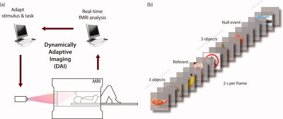
A schematic of DAI (a) and the timeline of the stimuli presented to volunteers (b). [Color figure can be viewed in the online issue, which is available at wileyonlinelibrary.com.]

METHODS

Overview of Method

For each fMRI acquisition, a referent object was chosen. DAI‐SS was then used to characterize what features of this referent object were most strongly encoded in the pattern of BOLD activity in a ventral ROI (Fig. 2). To do this, the pattern of response evoked by the referent stimulus was compared to that evoked by the other objects using online MVPA. Initially, 91 objects were presented sequentially in random order, interleaved with occasional referents and null events (Fig. 1b). Those evoking the most similar activity pattern to the referent were then presented again, and this procedure repeated. After five iterations it converged upon a “neural neighborhood” (NN) of the 10 items that evoked the most similar response. This NN could then be used to characterize feature selectivity in the neighborhood of the respective referent object. If, for example, the color of the referent object is strongly represented within its pattern of activity, then the NN of objects evoking a similar pattern of activity will comprise those that share the referent's color.

Figure 2.

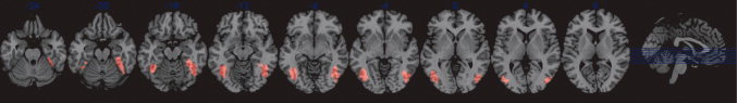
The ventral visual region used for adaptive imaging. [Color figure can be viewed in the online issue, which is available at wileyonlinelibrary.com.]

Choice of Referents

We measured feature selectivity in the neighborhoods of three different referents. First, to validate the procedure, we used a face referent. Our ROI included a portion of the fusiform gyrus (although it skirts FFA), and we expected the NN to show selectivity for faces, a semantic feature [Kanwisher et al.,1997]. We present one main and two supplementary analyses using this face referent, to provide a measure of consistency. A second referent, a zucchini, was chosen as it fell on the opposite side of the representational space in Kriegeskorte et al.'s [2008] study. The third experiment generalized to a different stimulus set, and used a bird (owl) as a referent, which was complex and animate, but not dominated by a face.

Participants

All participants were healthy young adults (age‐range: 18–35) with normal or corrected‐to‐normal vision. Thirteen participants (four men) performed acquisitions for the face referent, 10 (four men) for the zucchini referents, and 12 (two men) for the owl referent. Two additional experiments using a face referent are reported in the supplementary materials to allow the reader to evaluate the degree of consistency of feature tuning as measured with the DAI‐SS procedure. These each contained 20 participants.

Stimuli

Visual stimuli were presented using DirectX on a Windows PC running VB.net 2008 Express Edition, back‐projected onto a screen behind the participants' head and viewed through a mirror. Images were presented in the centre of the screen, scaled to fill an invisible square bounding box of around 3° of visual angle, for 2 s, followed by a fixation cross for 2 s. Three stimuli were presented sequentially, followed by a referent, another three stimuli and a null trial comprising a blank gray screen for 4 s (Fig. 1b).

For the experiments that used the face and zucchini referents, the stimuli were 92 pictures of objects from Kriegeskorte et al. [2008], presented on a mid‐gray background. This set was designed by Kriegeskorte et al. to be approximately half (52%) animate (here self‐propelling living objects, including faces, human bodies, and animals) with the remainder inanimate (artificial objects and static natural objects, e.g., a tree). The alternative picture set used for the owl referent comprised 385 pictures taken from Acres et al. [2007], presented on a white background. They were approximately half (48%) living (no human faces or body parts but many kinds of animal) and half non‐living objects. Four non‐overlapping sets of 91 objects were distributed across the participants. In each acquisition, the set of objects was searched to find those that evoked the most similar pattern of neural activity to the referent.

Task

For the face and zucchini referents, participants were asked to remain still and watch the stimuli, and were told their movements and brain activation were being assessed in real time. For the owl referent, a simple task was used to encourage the maintenance of attention—participants were asked to press one of two buttons to indicate whether the picture on the screen was “round” versus “long and thin.”

MRI Acquisition

All scanning was performed using a Siemens 3T Tim Trio at the MRC CBU in Cambridge, UK. Functional magnetic resonance imaging (fMRI) acquisitions used EPI (TR = 1 s, TE = 30 ms, FA = 78°) with a matrix size of 64 × 64 and in‐plane voxel size of 3 × 3 mm. There were 16 slices with a rectangular profile that were 3 mm thick and separated by 0.75 mm. They were oriented to tip down anteriorly, and cover both V1 and the inferior surface of the occipital and temporal lobe. Each began with 18 dummy scans during which a countdown was shown to the volunteer. An MPRAGE sequence (TR = 2.25 s, TE = 2.98 ms, FA = 9°) was used to acquire an anatomical image of matrix size 240 × 256 × 160 with a voxel size of (1 mm)³. Structural and functional data analyses were done in real‐time.

ROI

The ROI was defined using a functional localizer that identified object‐selective cortex [Malach et al.,1995] in an independent study with 15 participants (Lorina Naci, PhD dissertation, University of Cambridge). The ROI was derived by contrasting the BOLD response evoked by masked objects to that evoked by a baseline comprising the masks alone. Colored images of familiar objects and 3D abstract sculptures were presented briefly (17 ms), interposed between a forward mask (67 ms) and a backward mask (133 ms). The masks for each object were derived from phase‐scrambling the image of that object. In the baseline trials, instead of an object, an empty white display was presented interposed between two masks. The BOLD data for this localizer were thresholded at P < 0.001 uncorrected. The ROI encompassed ventro‐lateral occipital regions and extended anteriorally into a lateral fusiform region of inferior temporal cortex (Fig. 2).

DAI‐SS

An evolutionary algorithm was used in which objects were iteratively selected in multiple “generations.” Each run of adaptive imaging was broken into five generations. In the first generation, all 91 stimuli were presented once in a random order, interleaved with the referent and null trials as described above. At the end of the generation, there was then a 24 s gap in which a message “There follows a short pause...” was shown until 4 s before the recommencement of the next generation of object images. During this time, real‐time MVPA analysis was performed to identify the objects that evoked the most similar pattern of neural activity to the referent. The MVPA method used Spearman correlation to compare the spatial pattern of the parameter estimates in the ROI for the referent with that for each of the other objects. Like others [Haxby et al.,2001; Kriegeksorte et al.,2008] we have found the distance metric of correlation to be effective for MVPA. In the second generation, the 24 most similar items (i.e., highest correlation values) were presented, and the procedure was iterated. The generation sizes were 91, 24, 20, 16, and 13 objects. The number of generations and their size was optimized by simulations prior to the experiments.

Real‐Time Neuroimaging Analysis

Real‐time analysis software was written using Matlab 2006b and components from SPM 5, and is freely available with an open‐source license. It was run on a stand‐alone RedHat Enterprise 4 Linux workstation. The real‐time analysis system implements image pre‐processing and statistical modeling, as well as DAI in which the ongoing fMRI results are used to contingently modify the stimulus list.

In the real‐time system, an event handler triggered the appropriate actions as fMRI data arrived. When an anatomical image was received, it was converted from DICOM to NIFTI and normalized to the MNI template. This was used to derive the back‐normalization from standard space where the ROI was specified, to the individual subject's brain. On receipt of an EPI, this ROI was re‐sliced to the native space of the EPI, for use in subsequent analysis. The EPI images were motion‐corrected and high‐pass filtered (cutoff 128 s).

At the end of each generation, the data from the ROI were extracted and modeled using linear regression. Each of the 92 object regressors was formed from 2‐s‐long boxcars starting at the onset of each presentation of that object, convolved with the canonical hemodynamic response as defined by SPM. To remove noise, additional “spikes and moves” regressors were included to model out scans that relative to the previous scan had abrupt movements (>0.5 mm of translation or >1 degree of rotation along any of the x, y, and z axes) or changes in global signal (sum of squared difference between images is more than 1.5% of the globals squared). We have found this strategy to be more effective for fMRI studies in which the volume acquired is small (as here, with only 16 slices). If a big portion of the small volume is functionally responsive, BOLD activity due to the paradigm can influence the motion estimation. In this circumstance, using a traditional strategy of modeling out all effects that correlate with the realignment parameters removes valuable signal. In contrast, BOLD activity alone cannot trigger the introduction of spikes and moves regressors, making this method more robust.

As the parameter estimates of the object and referent were calculated across all generations acquired to that point in the imaging run, it was possible for objects not to be selected for one generation, but then re‐enter in the next generation. Following the final generation, the 10 most similar items were selected as the “neural neighborhood” (NN) of the referent.

Offline Analysis of Consistency and Feature Tuning

To test for the consistency of the NNs across participants, a permutation test was performed. This examined whether some items were selected for the NN more frequently than would be expected by chance. To model the data under the null hypothesis, in each permutation 10 items were selected at random without replacement from 91. We created separate simulations for each participant (N = 13 or N = 12) and generated a group level measure by identifying the 10 items that occurred most frequently across the simulated participant data. As a summary statistic, we calculated the mean occurrence frequency of these ten items. This was repeated 40,000 times to obtain a distribution of the statistic. The same statistic was calculated for the actual experimental data and compared to the distribution to obtain the P value of this value occurring by chance under the null hypothesis.

The sensory features extracted from each image are illustrated in Figure 4 and listed in Table I. In addition to these feature values that were derived for individual images, a measure of the pairwise similarity of the shape of the referent to each image was calculated using a Gabor jet model similar to that used by Kim et al. [2009]. Following down‐sampling to an ∼60 × 60 pixel grid, each image was fit with a set of multi‐scale Gabor jets centered on each point in a 9 × 9 grid spanning the image. Each jet comprised Gabor functions (extending to 3 s.d. of their envelope) at eight orientations and across five logarithmically spaced wavelengths (pi/8 to pi/2), giving 40 Gabors per grid point. The Gabor model was fit to each image using linear regression, and the pairwise dissimilarity between images defined as the sum of the squared difference of their Gabor coefficients, normalized through division by the product of the magnitudes of the Gabors of each of the images.

Figure 4.

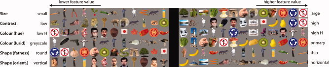
Sensory features illustrated with stimuli from set containing the face and vegetable referents. The lowest‐ and highest‐valued 12 objects are shown for each feature dimension. [Color figure can be viewed in the online issue, which is available at wileyonlinelibrary.com.]

Table I.

Derivation of perceptual features

Feature	Derivation
Size	Number of pixels
Contrast	Mean of sum of squared difference of each color channel from background color
Color (hue)	H value of mean color in HSV space
Color (lurid)	Mean of standard deviation across RGB for each pixel
Shape (thin)	Ratio of eigenvectors from Cartesian coordinates of occupied pixels
Shape (horizontal)	Thinness multiplied by orientation transformed into upper right quadrant (0 = horizontal, pi/2 = vertical)

Calculations performed on all pixels that were not the background color.

The semantic features for each picture set reflected their main sub‐categories with more emphasis on the types of objects used as referents (a face, zucchini, and an owl). For the set of objects from Kriegeskorte et al. [2008] we used their distinction into nearly equal animate versus inanimate groups and then classified by human, face, fruit, or vegetable. For the Acres et al. [2007] set, we used their classification into nearly equal living versus non‐living groups, and of the former into categories prominent in the set: bird; mammal‐amphibian; and other animal groups. There were human bodies and faces in Kriegeskorte et al. [2008] but not Acres et al. [2007].

For each acquisition, across the set of 91 objects (excluding the referent) the features were standardized to a z score. In each experiment, for each subject we took a mean of each feature across the 10 items in the NN. If object selection were random, the expected value of the mean of every feature across the NN would be zero. Statistics were calculated using a one‐sample t test across subjects.

We also tested whether the features for which selection was found in the NN of a given referent had more extreme values in that referent. To do this, we identified two groups of features—those for which selection was found (from the one‐sample t tests in the last paragraph) and those that were not. We then compared the magnitude of the referent's feature values between these two groups using a two‐sample t test.

Relating Groups of Features to NN Using a Classifier

We used a linear‐discriminant classifier to assess the effectiveness with which a set of features describing an object could be used to predict whether that object would make it into the NN. For each referent, a classifier was trained to discriminate objects that were selected for the NN from those that were not, on the basis of their feature vectors. A leave‐one‐out strategy across subjects was used, with training performed on all but one subject and the classifier's performance was then tested on the remaining subject. To quantify the importance of different kinds of information in determining a NN, three feature sets were used: (1) all of the features; (2) only the sensory features; and (3) only the semantic features. A repeated‐measures ANOVA with factors “subset type” (all/sensory/semantic) and “referent” (face/zucchini/owl) was then used to assess the classification performance.

Model‐Free Feature Analysis

Principle Component Analysis was used to identify the components that underlay the spatial patterns across the 92 objects. To provide the input data for this, a new GLM was set up using SPM to model just the responses to the first generation of adaptive imaging (i.e., a single presentation of each object). This was done for the two sessions that used the Kriegeskorte et al. [2008] stimuli, with the face and zucchini referent. Following PCA on the beta maps for each object, the distribution of the magnitudes of the resulting components was examined for a “knee” inflection point, to provide an estimate of the dimensionality of the data.

To identify whether the principal components of the activation patterns originated neurally or were imaging artefacts, we applied a linear‐discriminant classifier to quantify whether the patterns varied in a way consistent with the object being shown to the participant. To do this, in all subjects for which we had multiple sessions (N = 12 with 3 sessions, N = 1 with 2 sessions) we performed a nested leave‐one‐out procedure across sessions and objects. In each iteration, a single session was allocated for testing and the remainder used to train a classifier. A single target object was chosen. The classifier was trained to distinguish from the activation pattern evoked by an object whether it was the target or a non‐target. Performance was evaluated using signal detection theory on recognition performance for the test block: we quantified hits (classifier identified as target a correct object) and false alarms (classifier identified as target an incorrect object), averaged these across all sessions in a subject, and then calculated d‐prime. This procedure was repeated with each of the objects chosen as the target in turn, and an average taken across objects for each subject. Statistics were then performed across subjects. This analysis was repeated first for just patterns formed from the first principle component, then the first two components, and so on, to obtain a measure of single‐object classification performance as a function of the number of components. The growth in classification performance with the number of components was quantitatively investigated. To increase SNR on what would be expected to be a noisy measurement, we averaged the d‐prime scores in groups of 6 (i.e., components 1–6, 7–12, 13–18, 19–24) and performed t tests between successive groups with subject as a random factor.

RESULTS

First, a human face was used as a referent (N = 12). DAI‐SS converged upon a NN that was consistent across participants (Fig. 3a), with some objects selected more frequently than chance (on average each object in the top 10 was found in the NN of 4.6/12 participants, permutation test, P < 0.0001) and others rejected more frequently than by chance (mean frequency of bottom half of objects 0.17/12, P < 0.0001). To identify what drove the selection of the items that comprised the NN, we quantified sensory and semantic features of each object, and standardized each feature to give zero mean and unit standard deviation across the objects in the initial stimulus set. Randomly selecting from this set would yield feature values that were distributed around zero. In contrast, in the NN, non‐zero values were observed along several feature dimensions, indicating selectivity (Fig. 5a, statistics from one‐sample t tests on graph and in Table II), most strongly along a number of semantic feature dimensions. In an additional analysis, in which face stimuli were excluded, tuning to animacy persisted, indicating tuning did not merely reflect a face‐selective response (Table II, right column). In summary, as predicted, there was strong tuning to faces.

Figure 3.

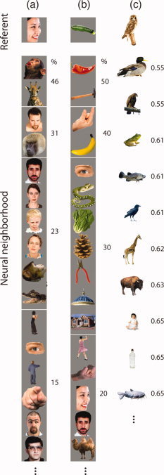
The neural neighborhoods (NNs) of the face (a), vegetable (b), and bird (c) referents. In columns (a) and (b), the items are ranked in order of the % of participants for which the item was found in the NN (top = most frequent). This measure could not be used for the bird referent as different stimuli were used across participants, and instead in column (c), we ranked the items by the similarity of the neural response they evoked to the referent (most similar is top item with low score on dissimilarity metric, see Methods). Note columns (a) and (c) are dominated by living objects. [Color figure can be viewed in the online issue, which is available at wileyonlinelibrary.com.]

Figure 5.

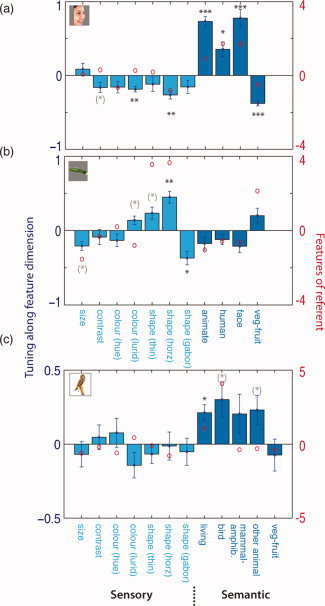
The features of the NNs following DAI Similarity Search (DAI‐SS) for the face (a), vegetable (b), and owl (c) referents (Mean ± one standard error). The asterisks denote the results of t tests for feature selectivity across subjects. Asterisks in black denote P values Bonferroni corrected by the number of features tested (*P < 0.05, **P < 0.01, ***P < 0.001), and those in gray the uncorrected significance (see also statistics in Tables II and III). The red circles show the feature values for each referent. [Color figure can be viewed in the online issue, which is available at wileyonlinelibrary.com.]

Table II.

Features of face and zucchini referents and their NNs

Feature	Face similarity (N = 13)			P a	Zucchini similarity (N = 10)			P a	Face versus zucchini
	Referent	NN mean	t (12)		Referent	NN mean	t (9)		t (21)	P a
Size	0.06	0.08	1.06		−1.57	−0.21	−3.53	(<0.01)	2.79	(<0.02)
Contrast	0.30	−0.16	−2.36	(<0.05)	0.31	−0.09	−0.84		−0.63
Color (hue)	−0.66	−0.16	−2.02		0.22	−0.13	−1.56		−0.23
Color (lurid)	0.27	−0.19	−4.86	<0.005	−0.81	0.14	2.48	(<0.05)	−4.96	0.001
Shape (thin)	0.19	−0.12	−1.23		3.88	0.23	2.83	(<0.02)	−2.67	(<0.02)
Shape (horizontal)	−0.83	−0.26	−4.71	<0.005	4.00	0.45	5.65	<0.005	−7.57	0.0001
Shape (gabor jet)	NAb	−0.16	−1.76		NAb	−0.37	−4.09	<0.05	1.66
Animate	0.96	0.73	11.6	<0.0001	0.60	−0.17	−1.93		8.50	0.0001
Human	1.71	0.35	3.60	<0.05	0.60	−0.12	−1.71		3.70	0.05
Face	1.71	0.78	6.63	<0.001	2.24	−0.21	−2.56	(<0.05)	6.48	0.0001
Veg–fruit	−0.46	0.38	−10.9	<0.0001	−1.74	0.20	2.03		−6.09	0.0001

^a P values in upright font are Bonferroni corrected for number of comparisons. P values in italics and parenthesis are uncorrected.

^bThe gabor‐jet measure is one of pairwise similarity between the referent and each object, and so does not have a meaningful value in isolation.

We then investigated why the NN for this referent reflected selection for particular features. Was it because the cortical region is tuned for some features but invariant to others, or was it determined by how the referent's features differed from other objects in the initial set? We compared the magnitude of the referent feature values for dimensions for which the NN was or was not selective. There was no significant difference, suggesting selection reflected neural tuning to specific features [t (9) = −1.03, ns].

With any new technique, it is reassuring to see replication. It is also informative in the current experiment to establish how sensitive the measurement of feature tuning is to the exact subset of stimuli, the configuration of the stimuli and the specific task. In two supplementary experiments, we repeated the DAI‐SS procedure for the face referent, but with new groups of volunteers and substantial differences in the stimulus set, stimulus configuration, and the task (Supplementary Methods). Despite these changes, similar feature tuning was obtained (Fig. S1), demonstrating the replicability and generalizability of the method.

Tuning Differs By Object Neighborhood

As discussed above, previous models have suggested that feature tuning should differ in the neighborhood of different objects. To test this, we ran DAI‐SS with another referent, a vegetable (N = 10), chosen as it evoked a highly distinct neural pattern in Kriegeskorte et al. [2008]. Again, consistency was found in the NN (Fig. 3b) across individuals (on average each object in top 10 occurred in 3.6/10 participants, P < 0.01 in permutation test; objects in bottom half in 0.19/10, P < 0.005). The NN reflected selectivity for several features, but along different dimensions to the face referent (Fig. 5b, Table II). As before, the distinctiveness of the referent's features was not related to the likelihood of them characterizing the NN [t (9) = 1.28, ns]. Directly comparing it with the face referent revealed NNs with different feature selectivities (see Table II, right column).

DAI‐SS was then run for a third referent, a bird (N = 12). We generalized to a stimulus set that was even broader and varied across participants [Acres et al.,2007]. The NN is shown in Figure 3c, and feature tuning in Figure 5c and Table III. The general consistency measure used for the other two referents could not be used because of the variation in stimulus set across participants but a separate measure was obtained from the classifier described later. The DAI‐SS procedure was effective for this new stimulus set, comprising 384 objects. Different patterns of feature tuning were found for this referent compared to the other two referents. The distinctiveness of the referent's features was again unrelated to the likelihood of them characterizing the NN [t (10) = −0.24, ns].

Table III.

Features of bird referent and its NN

Feature	Referent	NN mean	t (11)	P a
Size	−0.61	−0.07	−0.81
Contrast	−0.20	0.05	−1.67
Color (hue)	−0.59	0.08	0.78
Color (lurid)	0.44	−0.14	−1.67
Shape (thin)	−0.11	−0.07	−1.07
Shape (horizontal)	−0.80	−0.01	−0.13
Shape (gabor)	NAb	−0.05	−0.55
Living	1.05	0.21	3.96	<0.05
Bird	4.08	0.30	2.51	(<0.05)
Mammal/amphib.	−0.38	0.20	1.54
Other animal	−0.32	0.23	2.36	(<0.05)
Veg–fruit	−0.40	−0.073	−0.68

^a P values in upright font are Bonferroni corrected for number of comparisons. P values in italics and parenthesis are uncorrected.

^bThe gabor‐jet measure is one of pairwise similarity between the referent and each object, and so does not have a meaningful value in isolation.

Additional Supporting Information may be found in the online version of this article.

Relating Groups of Features to NN Using a Classifier

The classifier was able to relate the features to the NN reliably, but based on different balances of sensory and semantic features for the different referents (Fig. 6). A mixed‐effects ANOVA for the two referents (face, zucchini) probed with the same objects using a within‐subject factor of feature subset type (perceptual or semantic) and a between‐subjects factor of referent showed a subset by referent interaction [F (1, 21) = 17.3, P < 0.001] and a main effect of subset [F (1, 21) = 4.53, P < 0.05], but no main effect of referent [F (1, 21) = 3.56, ns]. A more general ANOVA including all three referents (face, zucchini, or owl) similarly yielded a subset by referent interaction [F (2, 32) = 6.90, P < 0.005], an effect of subset [F (2, 32) = 8.98, P < 0.005], and no effect of referent [F (1, 32) = 3.03, ns]. The robust subset by referent interactions show that sensory and semantic features contributed to different extents to the neural tuning around the different referents.

Figure 6.

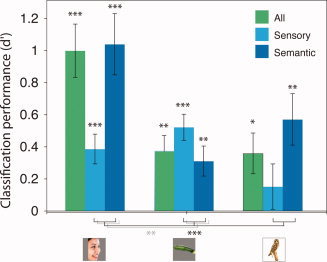
The performance of a linear‐discriminant classifier in predicting each referent's NN from different subsets of features. [Color figure can be viewed in the online issue, which is available at wileyonlinelibrary.com.]

Model‐Free Feature Analysis

We found no single feature that could account for tuning across referents. However, some feature not included in our analysis might more simply explain the results. To address this, we conducted further analyses that were agnostic about which features the region encodes, but focused upon how many. The patterns of neural response evoked by each of the 92 objects were entered into a Principal Components Analysis (PCA) to find the key modes of spatial variation. The scree plot (Fig. 7) shows the magnitude of each of the components. The inflection in this plot can be taken as an estimate of the dimensionality of the data, and suggests at least 20–25 distinct activation patterns, perhaps corresponding to at least 20–25 features.

Figure 7.

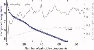
Magnitude of principle components (blue, left axis)—the knee provides an estimate of the neural activation patterns' dimensionality. To test whether these components provide functional information about brain activity, or merely imaging artifacts, a classifier was trained to distinguish the neural patterns of single objects from all of the other objects in a leave‐one‐out fashion. As the number of principle components used for the neural patterns increased, the performance of the classifier also increased, showing these components add useful information (dark blue, right axis). [Color figure can be viewed in the online issue, which is available at wileyonlinelibrary.com.]

As a greater number of principal components were used object classification performance increased, showing that the components were not imaging artefacts, but instead carried information about the stimulus. Classification performance reached an asymptote at around 20–25 components, suggesting that until this point the components carried useful information for stimulus discrimination, and independently supporting the lower bound on the number of features estimated from the scree plot. To improve SNR, the results were grouped into sets of six components and averaged within each subject. As illustrated in the top left of Figure 7, the comparison components 1–6 and 7–12, 7–12 and 13–18, and 25–31 and 32–37 all reached significance (all P < 0.05).

DISCUSSION

DAI‐SS and PCA revealed that visual representations of naturalistic objects in ventral cortex are multidimensional, with selectivity to combinations of semantic and sensory features differing by NN. More specifically, the NN of the face and owl referents is characterized by relatedness in semantic features, while the NN of the zucchini referent is characterized by relatedness in sensory features. This might reflect the pattern of tuning in the feed‐forward pathway, or differing extents of evolution in predictive coding or competition. In these frameworks, perceptual information is initially encoded, but becomes suppressed as semantic representations emerge at later stages in a processing hierarchy. It might also be that the difference in tuning across NNs is a result of different neuro‐cognitive processes being recruited to analyze different kinds of objects. Specific processes have been proposed, for example, for living things [Taylor et al.,2007], for faces [Tsao et al.,2006], and for stimuli for which we have developed expertise [Tarr and Gauthier,2000]. Perhaps, the face and owl referents engage specific modes of perceptual analysis, or exogenously evoke a greater depth of processing, than the zucchini referent. Future work with even larger object sets could more precisely characterize NNs, identify the key cognitive processes, the basis functions used to represent object space, and the neural structure of the code (e.g., local, sparse, or distributed).

Our results provide little evidence that task modulates the feature selectivity of the region. For the first referent, we obtained similar results for passive viewing and two replications with a memory task. For the third referent (the bird) participants were asked to perform a simple perceptual task (round vs. thin/long), but despite this we found greater tuning for semantic features, suggesting that some or all of the response may not be modulated by task. We have collected further data (to be reported elsewhere) that supports the view that this ROI is only weakly task dependent. It might be that more anterior temporal or frontal regions are the primary sites of task modulation. Those regions might selectively encode the task relevant features in any given context, as in the model of “adaptive coding” [Duncan,2001]. Alternatively, it is possible that task does change the neural response even in the more posterior regions we studied, but the changes are of a form that cannot be detected with fMRI or with MVPA (e.g., in sub‐second timing or the sub‐millimeter neural pattern).

A limitation of studies relating object features to neural representation is that they require the a priori construction of features that might be important. The current study has attempted to relax this limitation in two ways. First, DAI‐SS has allowed many features to be investigated simultaneously, reducing the requirement for a priori selection common in conventional designs that probe just one or two features. Second, we have conducted model‐free feature analyses using PCA. However, we have not investigated all possible features, and the power of any experiment to detect the effect of a feature is determined by the degree of variability in the stimulus set used. DAI is less constrained, but it is not without any limitations.

Although naturalistic stimuli were used in the current study, to address concerns that results from abstracted stimuli may not always generalize, it would be entirely possible to use DAI with abstracted stimuli. Indeed, an analogous method was used to great effect by Yamane et al. [2008] who investigated the representation of three‐dimensional shapes in monkey inferotemporal cortex by using electrophysiology. In their adaptive paradigm, a genetic algorithm was used to select stimuli that evoked the maximal response. An advantage of using adaptive methods with abstracted stimuli is that new stimuli can be generated online on the basis of imaging results, allowing an even larger stimulus space to be explored. Future experiments might use DAI to try to relate neural tuning for given natural referent stimuli and artificial stimuli, to more specifically identify what stimulus characteristics influence selectivity profiles.

Although DAI experiments focus on the measurement of particular parameters (here, multidimensional feature selectivity), this optimization does not come without certain trade‐offs. An important trade‐off of the current adaptive imaging method, DAI‐SS, is that only one ROI is characterized. As the stimuli are modified on the basis of the patterns evoked in this region, it is not possible to calculate retrospectively after an acquisition what would have happened had a different region been chosen. Also, it is not straightforward to interpret results from other parts of the brain using conventional imaging analyses, as the stimuli have been chosen on the basis of a response in the target region. In the current paradigm, for example, it would be interesting to assess feature selectivity in sub‐regions of our ventral ROI. These questions could however be addressed with further DAI‐SS experiments. Another trade‐off of DAI‐SS is that it characterizes selectivity in the region of a single stimulus, rather than for the entire stimulus space as representational similarity analysis does [Kriegeskorte et al.,2008]. Of course, in some circumstances (like the current investigation), the specificity of this characterization is a strength.

These trade‐offs point to areas of future developments for the DAI technology. Other methods of using DAI could have different patterns of costs and benefits. DAI paradigms might search out brain regions that respond in a similar manner, or search out features that are most important across the whole stimulus space. An ever‐present danger in neuroimaging, particularly in newer domains of investigation (like cognitive and social neuroscience) where structure‐function mappings are less constrained, is that experiments are designed to test narrow hypotheses that perpetuate existing models. By allowing more data‐driven and less paradigm‐constrained designs, DAI has the potential to allow theory to break out of cycles of circularity and encourage the development of innovative new models. We expect many new adaptive imaging paradigms will be developed to tackle particular questions.

Supporting information

Additional Supporting Information may be found in the online version of this article.

Supporting Figure 1 Figure S1. The features of the NNs following DAI Similarity Search (DAI−SS) for two experiments using a face referent and multiple stimuli (1, 2 or 3), plotted in a similar way to Figure 3 (mean +/− one standard error). The features are as for the previous experiment, except that the shape (Gabor) measure was not available. The top panel shows the features when multiple objects in a display were the same (N=20) and the bottom panel when they were all different (N=20). Note that the results are similar to those in Figure 3, although there is potentially a little less power to detect semantic features with the mixed displays.

Supporting information

REFERENCES

- Acres K, Stamatakis EA, Taylor KI, Tyler LK ( 2007): How do we construct meaningful object representations? The influence of perceptual and semantic factors in the ventral object processing stream. J Cogn Neurosci 19. [Google Scholar]
- Barense MD, Henson RN, Lee AC, Graham KS ( 2011): Medial temporal lobe activity during complex discrimination of faces, objects, and scenes: Effects of viewpoint. Hippocampus 20: 389–401. [DOI] [PMC free article] [PubMed] [Google Scholar]
- Drucker DM, Aguirre GK ( 2009): Different spatial scales of shape similarity representation in lateral and ventral LOC. Cerebral Cortex 19: 2269–2280. doi: 10.1093/cercor/bhn244. [DOI] [PMC free article] [PubMed] [Google Scholar]
- Duncan J ( 2001): An adaptive coding model of neural function in prefrontal cortex. Nat Rev Neurosci 2: 820–829. doi: 10.1038/35097557. [DOI] [PubMed] [Google Scholar]
- Haxby JV, Gobbini MI, Furey ML, Ishai A, Schouten JL, Pietrini P ( 2001): Distributed and overlapping representations of faces and objects in ventral temporal cortex. Science 293: 2425–2430. doi: 10.1126/science.1063736. [DOI] [PubMed] [Google Scholar]
- Kanwisher N, McDermott J, Chun MM ( 1997): The fusiform face area: A module in human extrastriate cortex specialized for face perception. J Neurosci: Off J Soc Neurosci 17: 4302–4311. [DOI] [PMC free article] [PubMed] [Google Scholar]
- Kim JG, Biederman I, Lescroart MD, Hayworth KJ ( 2009): Adaptation to objects in the lateral occipital complex (LOC): Shape or semantics? Vis Res 49: 2297–2305. doi: 10.1016/j.visres.2009.06.020. [DOI] [PubMed] [Google Scholar]
- Kriegeskorte N, Mur M, Ruff DA, Kiani R, Bodurka J, Esteky H, Tanaka K ( 2008): Matching categorical object representations in inferior temporal cortex of man and monkey. Neuron 60: 1126–1141. doi: 10.1016/j.neuron.2008.10.043. [DOI] [PMC free article] [PubMed] [Google Scholar]
- Lawson R, Powell S ( 2010): How do we classify everyday objects into groups? Presented at the Experimental Psychology Society, Manchester. [Google Scholar]
- Malach R, Reppas JB, Benson RR, Kwong KK, Jiang H, Kennedy WA, Ledden PJ ( 1995): Object‐related activity revealed by functional magnetic resonance imaging in human occipital cortex. Proc Natl Acad Sci USA 92: 8135–8139. [DOI] [PMC free article] [PubMed] [Google Scholar]
- Op de Beeck HP, Torfs K, Wagemans J ( 2008): Perceived shape similarity among unfamiliar objects and the organization of the human object vision pathway. J Neurosci: Off J Soc Neurosci 28: 10111–10123. doi: 10.1523/JNEUROSCI.2511–08.2008. [DOI] [PMC free article] [PubMed] [Google Scholar]
- Quiroga RQ, Reddy L, Kreiman G, Koch C, Fried I ( 2005): Invariant visual representation by single neurons in the human brain. Nature 435: 1102–1107. doi: 10.1038/nature 03687. [DOI] [PubMed] [Google Scholar]
- Rolls ET, Tovee MJ ( 1995): Sparseness of the neuronal representation of stimuli in the primate temporal visual cortex. J Neurophysiol 73: 713–726. [DOI] [PubMed] [Google Scholar]
- Tarr MJ, Gauthier I ( 2000): FFA: A flexible fusiform area for subordinate‐level visual processing automatized by expertise. Nat Neurosci 3: 764–770. [DOI] [PubMed] [Google Scholar]
- Taylor KI, Moss HE, Tyler LK ( 2007): The conceptual structure account: A cognitive model of semantic memory and its neural instantiation. Neural Basis Semantic Memory 265–301. [Google Scholar]
- Tsao DY, Freiwald WA, Tootell RB, Livingstone MS ( 2006): A cortical region consisting entirely of face‐selective cells. Science 311: 670. [DOI] [PMC free article] [PubMed] [Google Scholar]
- Ullman S, Vidal‐Naquet M, Sali E ( 2002): Visual features of intermediate complexity and their use in classification. Nat Neurosci 5: 682–687. doi: 10.1038/nn870. [DOI] [PubMed] [Google Scholar]
- Yamane Y, Carlson ET, Bowman KC, Wang Z, Connor CE ( 2008): A neural code for three‐dimensional object shape in macaque inferotemporal cortex. Nat Neurosci 11: 1352–1360. doi: 10.1038/nn.2202. [DOI] [PMC free article] [PubMed] [Google Scholar]
Associated Data
This section collects any data citations, data availability statements, or supplementary materials included in this article.
Supplementary Materials