Detection and localization of hippocampal activity using beamformers with MEG: A detailed investigation using simulations and empirical data

Abstract

The ability to detect neuronal activity emanating from deep brain structures such as the hippocampus using magnetoencephalography has been debated in the literature. While a significant number of recent publications reported activations from deep brain structures, others reported their inability to detect such activity even when other detection modalities confirmed its presence. In this article, we relied on realistic simulations to show that both sides of this debate are correct and that these findings are reconcilable. We show that the ability to detect such activations in evoked responses depends on the signal strength, the amount of brain noise background, the experimental design parameters, and the methodology used to detect them. Furthermore, we show that small signal strengths require contrasts with control conditions to be detected, particularly in the presence of strong brain noise backgrounds. We focus on one localization technique, the adaptive spatial filter (beamformer), and examine its strengths and weaknesses in reconstructing hippocampal activations, in the presence of other strong brain sources such as visual activations, and compare the performance of the vector and scalar beamformers under such conditions. We show that although a weight‐normalized beamformer combined with a multisphere head model is not biased in the presence of uncorrelated random noise, it can be significantly biased in the presence of correlated brain noise. Furthermore, we show that the vector beamformer performs significantly better than the scalar under such conditions. We corroborate our findings empirically using real data and demonstrate our ability to detect and localize such sources. Hum Brain Mapp, 2011. © 2010 Wiley‐Liss, Inc.

INTRODUCTION

Neuroimaging of cognitive functioning, such as memory processes, requires detection of neuronal activity emanating from deep brain structures, such as the hippocampus. Numerous experiments spanning several imaging modalities including functional MRI (fMRI) and positron emission tomography (PET) have demonstrated involvement of the hippocampus in a wide range of memory‐related processes. For example, hippocampal activation had been detected during memory encoding and retrieval [Davachi and Wagner, 2002; Henke et al., 1997], working memory [Ranganath and D'Esposito, 2001], relational problem solving [Astur and Constable, 2004; Greene et al., 2006; Heckers et al., 2004; Meltzer et al., 2008; Moses et al., 2010; Nagode and Pardo, 2002], and spatial navigation [Astur et al., 2005; Iaria et al., 2003].

While many imaging modalities can be used to detect activity from deep brain structures, magnetoencephalography (MEG) and electroencephalography (EEG) are unique in being noninvasive techniques that can directly observe neuronal currents, thus providing millisecond time resolution, orders of magnitude higher than the time resolution of fMRI and PET. Unlike the electrical signals measured by EEG, the magnetic fields measured by MEG pass through the various head tissue and scalp relatively undistorted. The ability to track the source time course with such high resolution provides the means for examining the contributions of various frequency bands to the source power spectrum, allowing exploration of the underlying processes responsible for these neuronal currents. For example, θ‐band oscillations have been implicated in hippocampal activity using this technique [Cornwell et al., 2008; Tesche and Karhu, 2000].

A large body of empirical evidence has recently accumulated demonstrating the ability of MEG to detect signals from deep brain structures such as the hippocampus during a variety of memory processes such as memory encoding and retrieval [Breier et al., 1998, 1999; Papanicolaou et al., 2002; Riggs et al., 2009], working memory [Tesche and Karhu, 2000], prospective memory [Martin et al., 2007], relational problem solving [Hanlon et al., 2003, 2005; Moses et al., 2009], and spatial navigation [Cornwell et al., 2008]. However, the debate over these results continued as other experiments examining hippocampal activity with MEG yielded mixed results. For example, experiments that attempted to detect spontaneous epileptic discharges using MEG, while simultaneously recording them using subdural electrodes yielded mixed results [Mikuni et al., 1997]. Sources found to have low strength as recorded by the subdural electrodes were less likely to be detected by MEG, with only 13% of such sources detected when their signal strength was below 100 nAm. As epileptic discharges span source strengths over an order of magnitude higher than stimulus‐evoked sources [Stephen et al., 2005], this led some to believe that detection of stimulus‐evoked sources with MEG is unlikely. Such generalizations, however, are inaccurate as several distinctions exist between the detection of spontaneous brain activity and stimulus‐evoked activity.

In this article, we rely on realistic simulations of stimulus‐evoked activity to show that while smaller signals are more difficult to detect, when the design parameters and methodology are optimized, and in the context of group‐averaged stimulus‐evoked activity, signals below 10 nAm can be detected. We examined how the detectability and localization of hippocampal signals depend on several factors in addition to source strength, including random noise and brain noise backgrounds, the experimental design parameters such as the number of trials and the number of subjects, the analysis techniques, and, in particular, whether control conditions are used. We focused on the ability of the adaptive spatial filter combined with a multisphere head model to properly localize hippocampal signals in the presence of visual field backgrounds and carefully examined its biases in the presence of brain noise. We demonstrated that while the weight‐normalized [and hence, unit‐noise‐gain (UNG)] adaptive spatial filter combined with a multisphere head model is not biased in the presence of random noise, it can be biased in the presence of brain noise resulting in hippocampal activations being localized outside the hippocampal structure, particularly for small signals. We also conducted a comparison between scalar and vector beamformers and demonstrated that scalar beamformers have a higher failure rate in detecting hippocampal signals in the presence of visual fields. Finally, we applied our findings to real data and empirically demonstrated our ability to detect and localize hippocampal sources.

THEORY AND METHODS

Adaptive Spatial Filtering Formalism

Beamformers are based on the concept of spatial filtering, where the aim is to pass the signal from the location of interest while blocking signals from all other locations. The operator of a spatial filter is a weight vector, w(r), which when applied to the measurement vector creates a weighted sum representing an estimate of source activity from the desired location, r. A functional image, therefore, requires N such weight vectors, where N is the number of brain locations (voxels) in the image. For a brain location of interest, r, the source activity at time t is the output of the spatial filter and is given by

(1)

where b(t) is the measurement vector given by

(2)

for an MEG system with M sensors. In this article, we follow the convention that plain italics indicate scalars, boldface lower‐case letters represent vectors, whereas boldface upper‐case letters represent matrices.

Defining a lead field vector, l(r), as the output of the sensor array corresponding to a source of unit moment at location r, the desired effect of passing signals from location r _p while blocking signals from other locations requires that

(3)

where r _p and r _q represent any two distinct locations, and where for simplicity, we assume that a fixed source direction at each location has been determined. We return to this topic below where we consider a more general case.

In reality, it is impossible to satisfy Eq. (3) and fully attenuate all sources outside the spatial location of interest. The exercise of designing an optimum spatial filter, therefore, amounts to minimize the contribution from sources outside the location of interest. This is achieved either through a MV or least‐mean‐squares technique, and in all cases, the solution to this problem takes the form [Reddy et al., 1987]

(4)

where γ is a scalar whose value depends on the details of the method used, and R is the second‐order moment matrix about the mean (often referred to as the covariance matrix) given by

(5)

where 〈〉 indicates the expectation value.

The MV‐based beamformers find a set of weights, w(r), which minimize the variance at the filter output,

(6)

subject to a constraint; the choice of this constraint determines the beamformer properties in terms of location bias, resolution, and the presence of artifacts. One popular choice is the unit‐gain (UG) constraint, where the signal from the location of interest, r _p, is required to satisfy

(7)

to preserve the source magnitude. While this choice yields a good image resolution, it can be shown to be biased and can result in strong artifacts near the center. The constraint

(8)

on the other hand, results in the same high resolution and can be shown to be unbiased with no artifacts near the center [Sekihara et al., 2005], although it applies a variable gain to the source amplitude depending on its location. This type of beamformer is often referred to as a lead‐field (LF) constrained or array‐gain constrained. A third type of beamformer, the UNG beamformer imposes a constraint on the gain such that the weights satisfy

(9)

and results in no localization bias and significantly higher resolution than the other two constraints above.

The bias of the UG constrained beamformer has been corrected in the literature by dividing the source power by the noise power [Van Veen et al., 1997], resulting in a quantity described in units of pseudo‐z scores [Robinson and Vrba, 1999]. In the presence of uncorrelated random noise that is identical across all channels, this modification is equivalent to normalizing the weights so that

(10)

where σ${}_{\text{N}}^{\text{2}}$ is the noise variance and w _x represents either w _UG, w _LF, or w _UNG. It is worth noting that this normalization makes the UG beamformer or the LF normalized beamformer equivalent to the UNG constrained beamformer in terms of resolution and localization accuracy as

(11)

In terms of the constraints, this means that the normalization in Eq. (11) effectively removes the constraint in Eq. (7) [or Eq. (8)] and replaces it with the condition in Eq. (9). The performance of any adaptive spatial filter also depends on the parameters affecting the accuracy of the covariance matrix such as the frequency bandwidth and the integration time. For a detailed assessment of these parameters on the beamformer performance, we refer the interested reader to the recent publication by Brookes et al. [2008].

The minimization in Eq. (6) subject to the constraint in Eq. (7) can be shown to satisfy the condition in Eq. (3) for a limited number of point sources in the absence of noise and, hence, block signals from other locations. In the presence of noise, however, this minimization serves only to reduce interference from such signals even when considering only two point sources. Strong sources from other locations may still make significant contributions to the solution, a phenomena often termed leakage. Reddy et al. [1987] derived an expression for the power output of two fully uncorrelated point sources and showed that in the presence of noise, the complete blocking of signals from outside the location of interest may not be achieved. In this article, we will show how leakage presents a serious challenge for the beamformer when the source of interest is a weak source and other strong sources are present, by attempting to localize hippocampal activation in the presence of primary visual sources, a case that is typical in such experiments.

The solution to the optimization problem in Eq. (6) can be achieved using the method of Lagrange multipliers, which determines γ in Eq. (4) to be

(12)

for the UG constrained beamformer. The solution with the LF constrained beamformer has the same format with l(r) replaced by l′(r) in Eq. (4), where

(13)

The UNG constrained beamformer gives

(14)

The formalism presented so far assumes the source direction to be known and, hence, applies to a scalar beamformer for which the source direction is determined by a separate procedure. The techniques usually used to calculate the source direction, however, integrate over a wide time range often involving hundreds of milliseconds. As sources are typically active over a short range, this results in averaging over significant amounts of noise (instrumental noise, brain noise, and leakage) which may or may not be isotropic. This issue becomes particularly significant for small SNR sources. In addition, by integrating over a wide time range, one assumes that only one source with a constant orientation is active at a given voxel over the entire time range. Using a vector beamformer one can avoid such assumptions and biases by calculating the three components of the weight vector to track the three components of the source activity vector. However, as radial components of source activity inside a conducting sphere are not detectable outside the sphere, one can switch to spherical coordinates and track the tangential (θ and ϕ) components only. In this case, the weights, source activity, and forward solution are given by

(15)

(16)

and

(17)

respectively. The minimization in Eq. (6) and its constraint Eq. (7) now become

(18)

and

(19)

yielding the solution

(20)

In the analysis below, we use a spatiotemporal or “event‐related” weight‐normalized MV vector beamformer [Sekihara et al., 2001], where the weights are calculated using Eq. (20) and normalized as described in Eq. (10). The two components of the source activity at a given instant in time are calculated using Eq. (1) for each of the two orthogonal directions where b(t) is the trial‐averaged MEG data. Following the approach of Sekihara et al. [2001], the metric

(21)

is used to construct the functional images.

As beamformers are known to be susceptible to source interference due to temporal correlations, we implemented the coherent source suppression model proposed by Dalal et al. [2006], which relies on specifying additional constraints in deriving the beamformer weights. As shown in Eq. (3), the condition to block signals from outside the location of interest is not explicitly specified but rather one relies on the minimization in Eqs. (18) and (19) to achieve it. As this is not achieved in the presence of correlated sources, one can explicitly add constraints to demand it to be achieved. In particular, the constraints

(22)

and

(23)

are added to Eqs. (18) and (19), respectively, where r _i is the location of the interfering source. The solution to this constrained minimization problem takes the form [Sekihara, 2008]

(24)

where

(25)

and C is the composite lead field matrix given by

(26)

Implementations of this model can, therefore, allow the user to specify the location of the suspected correlated source to be suppressed or suppression point, r _i. The algorithm can then calculate the lead fields for the location of interest, as well as the location of the suppression point, to formulate the composite matrix [Eq. (26)], which in turn is used to calculate the weights [Eq. (24)]. When the precise location of the interfering source is not known a priori, or the source is expected to have a large spatial extent, a suppression region (i.e., a collection of adjacent suppression points) can be specified. In this case, constraints similar to those of Eqs. (22) and (23) are added to correspond to the locations to be suppressed, and the composite lead field [Eq. (26)] would have two additional columns per extra suppression point. As more suppression points are added, however, the number of degrees of freedom in the minimization is quickly reduced, hence, impacting the performance of the model. A detailed assessment of the performance of this model and its application to auditory and visual data can be found in Quraan and Cheyne [2010].

SIMULATIONS

To establish the ability to detect evoked deep brain activity, several sets of simulations were conducted under various conditions with simulated sources placed in the left and right hippocampus. In one set of simulations, uncorrelated random Gaussian noise was added to the field at levels typical in an MEG system (5 fT/√Hz). For the remaining sets, the noiseless simulations were added to real visual evoked field (VEF) data acquired from each of 15 subjects. This allowed the inclusion of the actual brain noise background as well as its variation across trials and subjects. As experiments examining deep brain activations (such as hippocampal activations) often use visual stimuli, the choice of embedding simulated sources in datasets obtained from VEF data represents a real case scenario, a condition vital to the evaluation of the detectability and localization accuracy of such signals. This is particularly the case when beamformers are used, as they can fail to effectively attenuate strong sources from outside the region of interest, resulting in leakage. In the case of hippocampal activity in the presence of visual activations, for example, the detected visual activation can be more than an order of magnitude larger than the hippocampal activation. Despite the primary visual activation being distant from the hippocampus (>50 mm away for a typical adult subject), strong leakage into the hippocampus is observed. We demonstrated this effect by placing simulated sources on the baseline of these VEF datasets at latencies sufficiently far from the visual activation (∼800 ms away from the stimulus onset) where brain noise and leakage effects are small, as well as at latencies close to the visual activation (∼200 ms away from the stimulus onset) where brain noise and leakage are strong (see Fig. 2).

Figure 2.

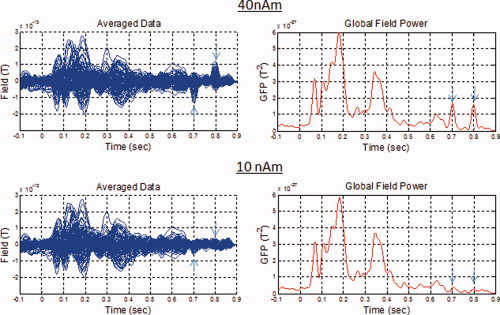
Channel‐by‐channel epoch‐averaged data and global field power from a VEF dataset of a single subject with simulated signals added to the data at ∼700 ms (right anterior hippocampus) and ∼800 ms (left anterior hippocampus) indicated by the vertical arrows. The simulated sources had a signal strength of 40 nAm (top) and 10 nAm (bottom). [Color figure can be viewed in the online issue, which is available at wileyonlinelibrary.com.]

The left and right hippocampal signals were simulated at latencies well separated in time to avoid temporal correlations that can negatively impact the performance of the beamformer. This is particularly important for weak sources where a small attenuation resulting from temporal correlations may cause them to fall below noise levels. We have previously shown, however, that some correlation–suppression models are partially effective at reducing interference effects between correlated sources, which would otherwise result in signal attenuation and localization inaccuracies [Quraan and Cheyne, 2010].

A simulated source was added to each subject's data, placed in the anterior hippocampus as determined from each individual subject's MRI. Each source was simulated as a 50 ms segment of a 10‐Hz sinusoid, with a source strength in the range of 10–40 nAm. Investigation of various datasets acquired within our neuroimaging group expected to evoke hippocampal activation, as well as information obtained from the literature [Kirsch et al., 2003; Martin et al., 2007; Tesche et al., 1996] showed the strength of reconstructed evoked hippocampal responses to be mostly below 30 nAm. Two publications have reported source strengths of up to 200 nAm (averaging at ∼100 nAm) in control subjects [Hanlon et al., 2003, 2005]. As one of our studies uses a similar paradigm and does not replicate these source strengths, we concluded that these very large source strengths are likely due to the localization model used. Source strengths in the range 100–200 nAm, however, were reported in hippocampal epilepsy, as expected in epileptiform discharges. As the radial component is practically undetectable by MEG, the MEG‐reconstructed source strength does not constitute the actual source moment but rather its tangential component. Hence, if a large component of the hippocampal source dipole moment is radial, the actual source magnitude may be much larger than what is detected with MEG. Furthermore, the neuronal current distributions within the hippocampus can lead to magnetic field cancellations at the position of the sensors due to the geometry of the hippocampus. As both of these effects are head‐geometry dependent, high subject‐to‐subject variability would be expected.

A survey of the literature [Hamada et al., 2004; Martin et al., 2007; Mikuni et al., 1997] showed various orientations for the localized hippocampal sources; however, for our simulations, we chose orientations similar to those obtained by Mikuni et al. [1997] as they were determined from epileptiform discharges and are, therefore, large enough to be reliably determined. These orientations were also reproduced by successive measurements, and the presence of signals was confirmed with simultaneous subdural electrode measurements. As these orientations are determined using MEG, they constitute the tangential component of the signal and, hence, in the absence of noise, the simulated source strength is entirely detectable.

To account for latency variability from subject to subject, the simulated signals were delayed by 2 ms in each subject relative to the previous subject, thus, covering a range of 30 ms for the 15‐subject datasets. All data were filtered to a band‐pass of 1–40 Hz and analyzed using a vector beamformer with a scanning resolution of 5 mm except where explicitly indicated. A multisphere head model fit to the inner skull surface of each subject's MRI was used to compute the forward solution. Images were generated for every sample then averaged over a 40 ms range encompassing all sources.

The VEF datasets were recorded during a colored‐pattern perception task that activates bilaterally symmetric sources in the visual cortex, using a 151‐channel CTF system (first‐order radial gradiometer system) and analyzed in a synthetic third‐order gradient configuration. The patterns were foveally presented for an interval of 200 ms with a random interstimulus interval between 1,250 and 1,500 ms. Each dataset contained 150 trials of 1,000 ms duration recorded at a sample rate of 625 samples/s. Coregistration of the MRI and MEG data was achieved by identifying the locations of the head localization coils on each subject's MRI. The origin of the coordinate system was calculated from these locations and a reconstruction grid was chosen to be large enough to encompass the whole brain. For group averaging, the functional images were first normalized to the MNI (T1) template brain (http://www.fil.ion.ucl.ac.uk/). Linear and nonlinear warping parameters were obtained from each individual's T1‐weighted MR scans then applied to the volumetric functional images to put each image in the Talairach stereotaxic space. A group average of these images was then computed for each condition and latency range.

Random Gaussian Noise

For the first set of simulations, only uncorrelated random Gaussian noise was added to the field at levels typical in an MEG system (5 fT/√Hz). By doing so, we avoided correlated brain noise, which may include strong sources that result in significant leakage into the hippocampus and may have thus impeded the detection and accurate localization of such sources. All other aspects of these simulations are otherwise equivalent to the simulations with brain noise, including the parameters of the simulation and the location of the simulated sources with respect to each subject's MRI (as discussed above), as well as all aspects of the analysis including head models. A comparison of simulations generated with random Gaussian noise and those with brain noise allowed us to quantify the effect of correlated brain noise and leakage on the detection and localization of hippocampal sources.

Group averages were computed for the random Gaussian noise scenario with sources simulated at strengths of 40, 30, 20, and 10 nAm. The group averages include all 15‐subject datasets with 150 trials/dataset. The hippocampal activation was detected and localized for all simulated source strengths, and the localization varied by a maximum of 6 mm among the four group averages. Figure 1 shows the localization error for each subject (defined as the Euclidean distance between the simulated source location and the detected source location) at 40 and 10 nAm. The localization error was also computed at 30 and 20 nAm then averaged over all subjects. At 40 nAm, the average localization error was 7.5 mm and went up to 10 mm at 10 nAm. To detect possible systematic biases, histograms of x, y, and z coordinate errors (e.g., X _error = X _{reconstructed} − X _simulated) were constructed. Small biases (of few millimeters) were observed and are within the errors expected from various sources of error such as head models.

Figure 1.

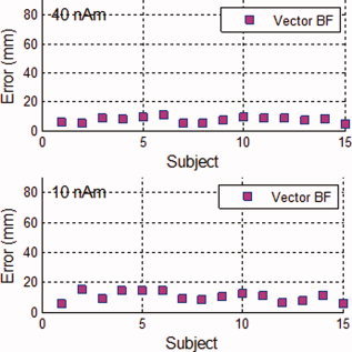
Localization error (defined as the Euclidean distance between the simulated hippocampal signal location and the reconstructed location) for each subject at 40 and 10 nAm, as labeled on each plot. Uncorrelated random Gaussian noise was added to the simulated signals at levels typical in an MEG system (5 fT/√Hz). [Color figure can be viewed in the online issue, which is available at wileyonlinelibrary.com.]

Low Brain Noise

For the second set of simulations, the simulated sources were placed in the latency range 800–830 ms following visual stimulus presentation, thus well after the VEF activity has subsided, to investigate the ability to detect and localize sources in the presence of low brain noise and weak leakage. Figure 2 shows the channel‐by‐channel trial‐averaged data as well as the global field power (GFP) for simulated source strengths of 40 and 10 nAm, confirming low brain noise in the latency range over which these sources were placed. While sources simulated with a strength of 40 nAm are visible on these plots, those simulated with a strength of 10 nAm cannot be distinguished from noise, even in this fairly low brain noise latency range. Simulations with source strengths of 20 nAm show similar results to the 10 nAm simulations, whereas those with 30 nAm are slightly above noise levels. Based on our studies, since many hippocampal signal strengths are below 20 nAm, they will not be visible on a GFP plot or a trial‐averaged data plot. Localization techniques capable of attenuating sources from outside the region of interest such as spatial filters, advanced multiple equivalent current dipole models, or other advanced techniques that are capable of localizing weak sources in the presence of strong backgrounds are therefore required to detect such weak sources. In the literature [Hamada et al., 2004; Hanlon et al., 2005; Tesche et al., 1996], many hippocampal activations were identified later than 300 ms relative to the visual stimulus onset, which represents a latency sufficiently far from the visual stimulus and comparable with what we simulate in this section.

Dependence on the signal strength

Figure 3 shows a group‐averaged glass‐brain plot of source activity in the Talairach coordinate system for sources simulated at 40, 30, 20, and 10 nAm, thresholded at 50% of the maximum. The group averages include all 15‐subject datasets with 150 trials/dataset. As can be seen from this figure, the hippocampal activation was detected and localized for all simulated source strengths, and the localization varied by a maximum of 7 mm among the four group averages. At 10 nAm, however, the signal to noise ratio is low resulting in the appearance of broad bands and artificial peaks that are likely driven by random noise and leakage.

Figure 3.

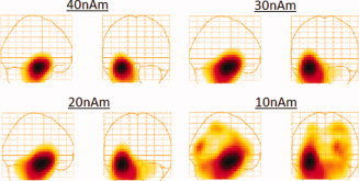
Group‐averaged functional images in the Talairach coordinate system of signals simulated at 40, 30, 20, and 10 nAm as indicated on the figures. The simulated signals were placed in the anterior hippocampus and added to VEF datasets obtained from 15 subjects at a latency sufficiently far from the active region (800–830 ms). [Color figure can be viewed in the online issue, which is available at wileyonlinelibrary.com.]

Dependence on the number of trials

To investigate the effect of the number of trials on the ability to localize such sources, we decreased the number of trials from 150 to 100, 50, and 10 trials and computed the group average for each of the four cases with a simulated source strength of 15 nAm. The choice of 15 nAm was based on estimates of hippocampal source magnitude from a 15‐subject dataset acquired using an n‐back paradigm which evoked hippocampal activity (see Application to real data). All 15‐subject datasets were used to construct the group average. Figure 4a shows a group‐averaged image for each case, where a subset of the 150 trials starting with trial 1 were used to construct the images. The hippocampal activation was detected and localized in all cases. Figure 4b shows the change in the peak location of the hippocampal activation as the number of trials is reduced (i.e., Euclidean distance between the peak location for each case and that for 150 trials). When only 50 trials were used the peak location changed by 11 ± 4 mm, where the error represents the standard deviation of three distinct sets of 50 trials. With only 10 trials the peak location changed by 18 ± 10 mm, where the error represents the standard deviation of five distinct sets of 10 trials. The increase in the standard deviation indicates the poor localization accuracy with reduced number of trials.

Figure 4.

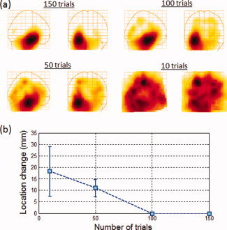
(a) Group‐averaged functional images in the Talairach coordinate system of signals simulated at 15 nAm. The simulated signals were placed in the anterior hippocampus and added to VEF datasets obtained from 15 subjects at a latency sufficiently far from the active region (800–830 ms). The images were constructed using 150, 100, 50, and 10 trials/dataset, as indicated on the panels. (b) Change in peak location of the reconstructed hippocampal activation as the number of trials were reduced from 150 to 10. [Color figure can be viewed in the online issue, which is available at wileyonlinelibrary.com.]

Dependence on the number of subjects

Figure 5 shows the change in position of the localized peak as the number of subjects is reduced from 15 to 12, 9, 6, and 3 subjects (i.e., Euclidean distance between the peak location for each case and that for the15‐subject group average). While the localization changed by <2 mm as the number of subjects was reduced from 15 to 12, a systematic increase in distance away from the 15‐subject group average is seen as the number of subjects is reduced below 12 reaching 7 mm for a group average of three subjects. The values for each group average were determined by computing the mean over several permutations of subjects (wherever possible, for example, there is only one permutation when all 15 subjects are used). The error bars are the standard deviations resulting from these permutations.

Figure 5.

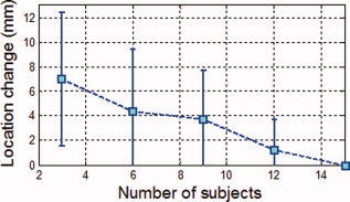
Change in peak location of the reconstructed hippocampal activation as the number of subjects is reduced below 15.

Although these results indicate that even six subjects are sufficient to localize hippocampal activations for the case at hand, we emphasize several issues here: (1) the purpose of choosing a large number of subjects is aimed at having a good representation of the population and guarding against biases from atypical activations that are specific to a single subject or a small subset of subjects; (2) although these simulations are modeled to mimic real data including trial‐to‐trial source amplitude variations, they do not take into account the likelihood that some subjects may perform the task poorly, and, hence, these results represent a best‐case scenario where all subjects are alert and performing the task properly; (3) if hippocampal signals are highly radial (and/or field cancellations occur due to the shape of the hippocampus), strong subject‐to‐subject variability would be expected due to variations in head geometry, and the hippocampal signal from some subjects may be too small to measure; and (4) in this set of simulations, we placed the signals at a latency sufficiently far from the active latency range to reduce brain noise effects. This may not be the case for some experiments, and the results from the next section where we tackle the more challenging case of the hippocampal activation being within the latency of the active visual sources may be more relevant.

Individual subjects

Finally, we examined the ability to localize hippocampal activations from individual subjects for this low brain noise latency range. The localization error (defined as the Euclidean distance between the simulated and detected position) for each of the 15 subjects for simulated sources at strengths of 40, 30, 20, and 10 nAm was computed for both the vector and scalar beamformers and plotted in Figure 6a. As the source strength decreased, the ability to properly detect and localize the simulated hippocampal signal decreased. Figure 6b (top) summarizes these results by showing the average of the localization error computed over all the subjects. For the vector beamformer, the averaged localization error increases from ∼15 mm at 40 nAm to ∼18 mm at 20 nAm, whereas the scalar beamformer results in an averaged localization error of ∼18 mm at 40 nAm increasing to ∼27 mm at 20 nAm. Figure 6b (bottom) shows the number of failures for both the vector and scalar beamformers as a function of simulated source strength, where a failure is defined to be a case where the localization error exceeds 20 mm. At 40 nAm, the vector beamformer fails 20% of the time, whereas the scalar fails 40% of the time. While the failure rate of the vector beamformer remains relatively unchanged as the simulated source strength is reduced to 20 nAm (∼20%), the scalar beamformer fails 47% of the time at 30 nAm and 60% of the time at 20 nAm. As the source strength is further reduced, the signal strength drops well below the background noise level, and both beamformers fail equally at identifying and properly localizing the sources.

Figure 6.

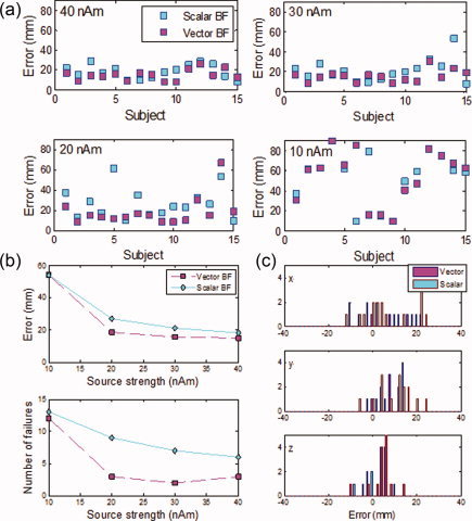
(a) Localization error (defined as the Euclidean distance between the simulated hippocampal signal location and the reconstructed location) for each subject where the signals were simulated at 40, 30, 20, and 10 nAm as labeled on each plot, then added to individual‐subject VEF data at a latency far from the active region (800–830 ms). Scalar and vector beamformers were used to perform the localization as indicated on the plot. (b, top) Localization error as a function of source strength averaged over 15 subjects (b, bottom) Number of localization failures for the same where a localization failure is defined as a distance error exceeding 20 mm. (c) Histograms of the localization error for the 40 nAm simulated source.

Under these conditions, the weak performance of the scalar beamformer relative to the vector beamformer is not surprising. As discussed in Section 1 of Theory and Methods, scalar beamformers rely on a determination of the source orientation and then construct only the component of the source activity in this direction. The source orientation is typically determined either through a grid search aimed at maximizing source power in each voxel [Robinson and Vrba, 1999] or through an eigendecomposition of the source power, where the largest eigenvalue is identified as the one corresponding to the source originating from that voxel [Sekihara et al., 2001]. The eigendecomposition method is essentially equivalent to the grid‐search method but achieves the purpose in a more computationally efficient fashion. In both methods, however, the power is calculated over a wide time range, typically spanning hundreds of milliseconds. Furthermore, the assumption is made that all activity determined by the beamformer to originate from a given voxel is indeed generated by brain sources originating at that location. For cases where the source of interest is weak and in the presence of other strong sources that result in leakage into the region of interest, as is the case in the problem at hand, this assumption fails. In other words, in such cases, most of the activity in the region of interest over a long time range results from leakage from strong sources outside the region of interest, and, hence, the determination of the source orientation using either of these methods is subject to significant errors. This error increases as the strength of the source of interest decreases, as is evident in Figure 6b from the increased failure of the scalar beamformer as the source strength is decreased. The scalar beamformer, therefore, ends up constructing the component of the source activity in a direction different from that of the source of interest and dismissing what might be a significant component of the source of interest. The vector beamformer, on the other hand, constructs the source activity in the two tangential directions, dismissing only the radial component which is typically small. We emphasize here, however, that in many applications of the scalar beamformer, the source of interest is the dominant one, and the effect of leakage is small or even negligible. In this case, an accurate determination of the source angle can be achieved, and the construction of the source activity component in only this direction is justified. However, constructing source activity of both tangential components even in such cases guards against dismissing unexpected components and provides verification that the source orientation was properly computed.

Although in the case of a weak source in the presence of strong leakage, the vector beamformer performs significantly better than the scalar, both beamformers give large localization errors, and so we proceeded to determine whether such errors constituted systematic biases in any particular direction or whether they were random. Figure 6c shows histograms of the localization error for each coordinate at 40 nAm. While the x coordinate shows a large random error, both the x and z coordinates show only small localization biases (few millimeters). The y coordinate (which corresponds to the Talairach x coordinate), however, shows a fairly large localization bias of ∼9 mm, in the lateral direction, toward the sensors. As the only difference between the simulations here and those in the previous section is the added brain noise (i.e., all other aspects of the datasets and head models are identical as well as the analysis techniques), this bias is partially driven by brain noise/leakage. In the next section, we lend further support to this conclusion by showing that the bias increases with increasing brain noise.

High Brain Noise

For the third set of simulations, the simulated sources were placed in the latency range 200–230 ms following visual stimulus onset, when VEF activity is still strong, to investigate the ability to detect and localize sources in the presence of high brain noise and strong leakage. In this latency range, typical hippocampal sources would not be visible on trial‐averaged data plots or GFP plots similar to those of Figure 2. We, therefore, attempted to detect such sources by localizing them using the beamformer then computing the group‐averaged images as we did above. As before, the images were averaged over 40 ms encompassing all sources.

Dependence on the signal strength

Figure 7a shows a group‐averaged glass‐brain plot of source activity in the Talairach coordinate system for sources simulated at 40, 30, 20, and 10 nAm for this latency range. The group averages include all 15‐subject datasets with 150 trials/dataset. As can be seen from this figure, the 40 nAm hippocampal activation was detected as the strongest activation but at 30 nAm, the primary visual activation was the strongest. Although hippocampal activation is still visible, a leakage pattern resulting from the activation of the visual cortices and extending all the way to the hippocampus is also visible. At 20 and 10 nAm, the hippocampal signal is no longer visible due to leakage from the primary visual sources. As most hippocampal signals are below the 30 nAm range, the ability to properly detect and localize small signals is crucial.

Figure 7.

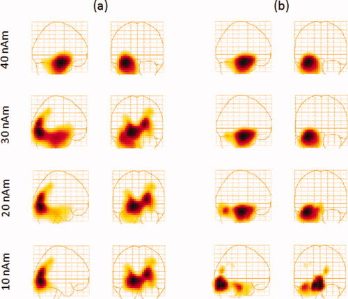
(a) Beamformer localization error averaged over 15 subjects for hippocampal sources simulated at various source strengths (as indicated on the figure), then added to individual‐subject VEF data at a latency within the active region (200–230 ms). (b) The same as in (a) but the images obtained from the control condition were subtracted from the experimental condition for each subject prior to averaging. [Color figure can be viewed in the online issue, which is available at wileyonlinelibrary.com.]

As the inability to localize such weak sources is due to beamformer leakage from the primary visual sources, if we are able to subtract out this leakage, we would be more likely to detect and localize hippocampal activations. The easiest way to achieve this is by designing experiments that include appropriate control conditions, where the condition of interest (which we will call the experimental condition) involves a task that is expected to activate the hippocampus, whereas the control condition involves a task that is not expected to involve the hippocampus system to the same degree. For example, for experiments that use visual presentations as stimuli, both the experimental condition and the control condition would include the visual activation. One can then construct experimental and control images and subtract them. As both images include the visual activation as well as its leakage patterns, ideally, subtracting the two would also subtract leakage from the primary visual sources that hindered the detection and localization of the hippocampal sources. Realistically, efficient subtraction of such sources relies on the way these control conditions are constructed and the number of trials used. One would expect the best subtraction of such leakage patterns to occur if the control trials were interleaved with the experimental trials, to ensure that the subject is responding to the visual stimuli similarly in both cases. In addition, interleaving ensures the capture of noise variations almost simultaneously for both conditions as well as any head movement variations. However, it is not always possible to interleave conditions because achieving the experimental condition may require separation from the control condition. In this case, one would have to subtract images constructed from individual runs (one run for the experimental and one run for the control), and while optimal leakage subtraction efficiency is not achieved, a reasonable subtraction efficiency can still be obtained as we demonstrate on both simulations and real data.

We constructed individual images for the 15 subjects from the VEF datasets discussed above, where simulated hippocampal signals were added (experimental), as well as 15 other VEF datasets acquired with the same subjects with no simulated hippocampal signal added (control). We then subtracted these images for every subject to obtain the experimental‐control (experimental minus control) images and constructed group–averaged images from those. Figure 7b shows the experimental‐control group–averaged images for simulated signal strengths of 40, 30, 20, and 10 nAm. As is the case with no control condition, hippocampal activation is successfully detected for the 40–20 nAm range. Furthermore, while at 10 nAm the primary visual activation is still present, its leakage patterns are effectively reduced, allowing the detection of the hippocampal signal. For such signals, however, the localization bias becomes fairly strong, as a result of the strong leakage and brain noise relative to the hippocampal signal, and the group‐averaged image shows hippocampal activation shifted laterally by 15 mm. As we have seen, this bias arises from the localization algorithm in the presence of noise and the subtraction of experimental‐control images does not eliminate this bias.

Dependence on the number of trials

To investigate the effect of the number of trials on the ability to localize such sources, we decreased the number of trials from 150 to 100, 50, and 10 trials, respectively, and computed the group average for each of the four cases with a simulated source strength of 15 nAm. All 15‐subject datasets were used to construct the experimental–control group‐averaged images. Figure 8a shows the group‐averaged images for each case where a subset of the 150 trials starting with trial 1 were used to construct the images. While the simulated signals were detectable even with only 10 trials, at such a low number of trials the beamformer bias is large, placing the simulated signal ∼18 mm away from the hippocampus. Figure 8b shows the change in the group‐averaged simulated signal localization as the number of trials is reduced. When only 50 trials were used, the peak location changed by 10 ± 4 mm where the error represents the standard deviation of three distinct sets of 50 trials. With only 10 trials the distance changed by 17 ± 13 mm where the error represents the standard deviation of five distinct sets of 10 trials. The increase in the standard deviation indicates the poor localization accuracy with reduced number of trials.

Figure 8.

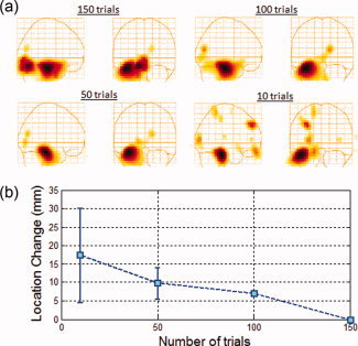
(a) Group‐averaged functional images in the Talairach coordinate system of signals simulated at 15 nAm constructed by subtracting the control condition from the experimental condition as shown in Figure 7b. The simulated signals were placed in the anterior hippocampus at a latency within the active region (200–230 ms) and added to visual evoked field datasets obtained from 15 subjects. The images were constructed using 150, 100, 50, and 10 trials/dataset, as indicated on the figures. (b) Change in localization as a function of trial number relative to 150 trials. [Color figure can be viewed in the online issue, which is available at wileyonlinelibrary.com.]

Dependence on the number of subjects

Figure 9a shows the change in position of the localized peaks on the group‐averaged experimental‐control images as the number of subjects is reduced from 15 to 12, 9, 6, and 3 subjects for a source strength of 15 nAm. While the localization error remained below 10 mm as the number of subjects was reduced from 15 to 12, a significant systematic increase in distance was seen as the number of subjects was reduced to 9 and reached 15 mm with only six subjects. As before, the values for each group average were determined by computing the mean over several permutations of subjects (wherever possible, for example, there is only one permutation when all 15 subjects were used). The error bars are the standard deviations resulting from these permutations. We note that the standard deviations are large even for 12 subjects and increase as the number of subjects is reduced. This indicates the wide variability between subjects and emphasizes the need for a large number of subjects to achieve localization that is not highly dependent on a specific subject (or a small subset of subjects). Furthermore, we note that a mean of ∼15 mm and a standard deviation of ∼5 mm, for example, indicate that for some subsets of six and nine subjects, the localization error can be quite large (a probability of 33% that the localization error will exceed 20 mm), indicating extremely poor localization in such cases. As an example, Figure 9b shows the group‐averaged experimental‐control images for 12, 9, 6, and 3 subjects for a single subset of subjects in each group. The general trend observed in this subset is generally common to other subsets, namely, with a large number of subjects the hippocampal and visual activations are the dominant ones (in this case the hippocampal activation being the strongest). As the number of subjects was reduced, other activations were seen, and with only three subjects the strength of the hippocampal signal observed was around or below the strength of other activations.

Figure 9.

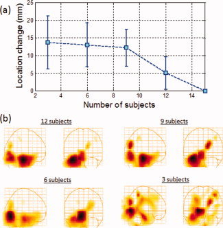
(a) Change in position of the localized peak as a function of number of subjects. The change in position is defined as the Euclidean distance between the peak location of each case and that of the 15‐subject group average. Simulated signals with a 15‐nAm strength were placed in the anterior hippocampus at a latency within the active region (200–230 ms) and added to visually evoked field datasets obtained from each subject. (b) Group‐averaged functional images in the Talairach coordinate system corresponding to the data in (a) constructed by subtracting the control condition from the experimental condition as described in Figure 7b. [Color figure can be viewed in the online issue, which is available at wileyonlinelibrary.com.]

Individual subjects

Finally, we constructed the functional images for the individual subjects. In only three of the 15 subjects was a hippocampal signal readily identified from these simulation images.

APPLICATION TO REAL DATA

In this section, we chose an example from real data where subjects were presented with a colored‐pattern perception task that activates bilaterally symmetric sources in the visual cortex. In one block (experimental), the subjects were asked to indicate whether the colored pattern presented to them was the same as the previous pattern by pressing a button. In the second block (control) similar patterns were presented, but the patterns did not repeat and the subjects were not asked to remember whether the pattern was identical to a previous one. The experimental condition is expected to elicit greater hippocampal activation than the control condition due to its greater explicit memory demand. The second block served as the control condition and was used to subtract out the dominant VEF activation and its leakage patterns as we discussed above.

The data were analyzed with the vector beamformer and group averages were constructed over 40 ms time ranges in a similar manner as discussed in the simulations section. A half‐interval (20 ms) sliding window was used over the range of 80 to 400 ms, resulting in 16 group averages. Statistically significant hippocampal activation was found in the 80–120 ms time interval when experimental‐control images were constructed in the same manner as was done in the simulations.

When no control condition was used, no hippocampal signals were observed. Figure 10a shows the experimental group‐averaged image for the range 80–120 ms at a threshold of 80% of the maximum peak where only primary visual activation is seen. Lowering the threshold to 50% (Fig. 10b) still shows no hippocampal activation, but the long‐ranged primary visual leakage patterns are dominant and stretch well into the hippocampus, thereby obscuring any possible hippocampal activation. To reduce these leakage patterns, we constructed the experimental‐control group–averaged image shown in Figure 10c plotted at a 50% threshold. Although the visual activation is still visible indicating limited subtraction efficiency, left hippocampal activation is clearly visible and is the only other significant activation in this time range throughout the entire head volume. To explore the possibility that a lack of a right hippocampal signal is due to the susceptibility of the beamformer to temporal correlations, correlation corrections were applied [Dalal et al., 2006; Quraan and Cheyne, 2010] but did not reveal the presence of a right hippocampal source.

Figure 10.

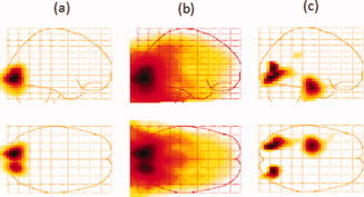
Group‐averaged image for the range 80–120 ms at a threshold of 80% (a) and 50% (b) of the maximum for a memory task known to activate the hippocampus. (c) Same as (b) but the control condition images were subtracted out from each subject's image before averaging. [Color figure can be viewed in the online issue, which is available at wileyonlinelibrary.com.]

We then looked at the images from the individual subjects. Of the 15 subjects, peaks in the proximity of the hippocampus region were found in only two. This is in‐line with what we have already seen in the simulation and indicates that the detected (tangential) component of the hippocampal signals were generally small (below 20 nAm). Figure 11 shows the functional images from the two subjects where hippocampal activation was observed. The peak for this activation for subject 1 corresponds to a source moment of 14 nAm and is within 10 mm of the hippocampus. The peak for subject 2 corresponds to a much lower source moment of only 5 nAm and results in much lower signal to noise ratio. As we demonstrated in the simulation, in such cases, the beamformer localizes the hippocampal signal to a location lateral to the hippocampus.

Figure 11.

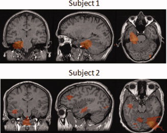
Functional images from those two subjects in which hippocampal activation was observed.

DISCUSSION AND CONCLUSIONS

Although MEG is often associated with the detection of superficial cortical sources, based on extensive realistic simulations, we have shown in this article that deep sources, such as the hippocampus, may also be detected with MEG using stimulus‐evoked activity, particularly when group averages are constructed. In this respect, and due to its superior time resolution, MEG can contribute to the understanding of such sources and the underlying mechanisms by exploring their time and frequency characteristics.

All the simulations we presented in this article are based on a first‐order radial gradiometer system with a 50‐mm baseline. Successful detection of hippocampal sources has been reported using this type of system [e.g.,Cornwell et al., 2008; Moses et al., 2009; Riggs et al., 2009] as well as planar gradiometer systems [e.g.,Hanlon et al., 2003, 2005; Tesche, 1997; Tesche and Karhu, 2000; Tesche et al., 1996]. In the work of Mikuni et al. [1997], where hippocampal signals were only detected 13% of the time in epileptic discharges when the signal strength was below 100 nAm, a planar gradiometer system was used. Such systems have a reduced sensitivity to deep sources [Hamalainen et al., 1993; Vrba and Robinson, 2001] compared to a radial gradiometer system with a 50‐mm baseline, which may partially explain the failure of some studies to detect deep sources. In the past and in the absence of effective noise reduction techniques, the use of planar gradiometers was largely driven by their efficient noise subtraction capabilities. More recent systems that use a planar gradiometer design also provide magnetometer channels that have even longer reach than radial gradiometer channels, thus complementing the planar gradiometer channels. Successful detection of hippocampal activation using these systems has been reported [Martin et al., 2007]. The effectiveness of magnetometer systems was very limited in the past due to their higher sensitivity to noise, particularly at sites where noise levels are high. More recently, several noise‐reduction mechanisms have demonstrated the ability to significantly reduce the noise levels, allowing magnetometer channels to be more effective. These noise‐reduction mechanisms include the design of active shielding where shielded rooms are equipped with large (feedback) coils installed in their walls to generate noise cancellation fields. Channels in the MEG system designed to measure the noise levels actively drive these coils to generate fields that counter (and thus reduce) the noise in these channels. At the software level, signal space separation methods have also been used where the part of the signal originating inside the MEG can be identified using solutions to Laplace's equation in spherical coordinates [Jackson, 1999; Taulu and Simola, 2006]. Such developments will significantly aid the effort to explore deep sources.

We have shown in this article that the ability to detect typical hippocampal signals by exploring peaks in stimulus‐evoked data averages or GFP spectra is unlikely, as such signals typically fall below the global noise levels. The use of spatial filters, on the other hand, which rely on attenuating signals from outside the region of interest (combined with optimized experimental design and analysis techniques), allows the detection of the tangential components of fairly weak signals. In this article, we used an event‐related vector beamformer with correlation suppression capability [Quraan and Cheyne, 2010] to detect hippocampal sources. We showed that the largest impediment in detecting hippocampal sources using beamformer techniques, in the presence of strong noise backgrounds, were leakage patterns that extend from the visual cortex into the hippocampus. For the specific case that we explored where stimulus‐evoked visual sources were present in the dataset, signals down to 30 nAm were detectable with such sources while those at 20 nAm and below were not. According to our estimates of hippocampal sources from various stimulus‐evoked paradigms designed to evoke activity in the hippocampus, most of these source strengths fall in the undetectable range in the presence of VEF sources. The threshold of detectable signals, however, becomes lower if the beamformer leakage is subtracted out. In this article, we used experimental‐control image subtraction to reduce the leakage, and showed that by doing so, and in the context of group‐averaged stimulus‐evoked activity, we were able to detect hippocampal signals below 10 nAm, which puts most hippocampal signals in stimulus‐evoked experiments within reach. The localization accuracy of the hippocampal signal, however, depends on the number of trials, and the change in the peak location of the reconstructed hippocampal signal relative to 150 trials increased as the number of trials was decreased exceeding 11 mm below 50 trials.

To generalize the results of a stimulus‐evoked experiment to the population considered with reasonable confidence, a sufficient number of subjects must be considered. However, the inclusion of a large number of subjects serves another purpose at the technical level. In the ideal case where all subjects' responses are identical, the increased number of subjects provides repeated measurements. As there is a finite probability that weak signals will not be detected, the repeated measurements provide higher probability that they will be detected as well as increased localization accuracy. Furthermore, as brain noise varies from subject to subject while the activation of interest is consistently present at some level in most (if not all subjects), averaging over a large number of subjects serves to enhance the activation of interest by reducing brain noise backgrounds. As a consequence, detection of weak activations in individual subjects is more challenging as we have seen in the case of the simulated hippocampal signal and the evoked hippocampal signal. For both simulations and real data, and with the localization modality we used (beamformer), the analysis technique (experimental‐control image subtraction), and the experimental design parameters (e.g., 150 trials), we were able to detect hippocampal signals in ∼20% of the subjects. As the ability to detect signals in individual subjects is crucial in clinical applications improving our localization modalities and analysis techniques will help extend clinical applications of MEG.

While the UNG beamformer combined with a multisphere head model has been shown to be unbiased in the presence of noise, a result arising from this analysis is that such algorithms can be significantly biased when localizing weak sources in the presence of strong brain noise backgrounds. For sources in the anterior hippocampus, this bias can exceed 15 mm in the presence of strong brain noise backgrounds, putting the sources at a location significantly lateral to the hippocampus. This emphasizes the need to evaluate the localization models under conditions comparable to real data to arrive at valid conclusions.

While the ability to detect hippocampal signals has been debated based on the weak nature of such signals, leading many to conclude that MEG is an unreliable method for conducting such experiments, we have shown that the detectability of such signals largely depends on the experimental design parameters, the analysis techniques, and the localization models. The weak nature of signals from deep sources does not necessarily imply that such signals are undetectable. We point to other quantitative fields that are able to accurately infer the presence of weak signals. For example, in the field of Nuclear and Particle Physics, extremely small signals embedded in high noise backgrounds have been successfully detected at high confidence levels, leading to the discovery of new particles and phenomena. In a recent and challenging experiment in which the first author was involved, signals were measured at accuracies of 1 part in 10⁴ [Jamieson et al., 2006; MacDonald et al., 2008]. Recent progress in the MEG field to properly quantify the mathematical models and test their performance will pave the way for MEG to play a wider role in neuroimaging. The analyses presented here is a step toward a better understanding of the detectability of deep sources and toward developing techniques that help to improve their localization. In future work, we hope to examine other localization modalities and analysis techniques that may further improve our ability to detect deep sources and reduce localization bias.

REFERENCES

- Astur RS, Constable RT ( 2004): Hippocampal dampening during a relational memory task. Behav Neurosci 118: 667–675. [DOI] [PubMed] [Google Scholar]
- Astur RS, St Germain SA, Baker EK, Calhoun V, Pearlson GD, Constable RT ( 2005): fMRI hippocampal activity during a virtual radial arm maze. Appl Psychophysiol Biofeedback 30: 307–317. [DOI] [PubMed] [Google Scholar]
- Breier JI, Simos PG, Zouridakis G, Papanicolaou AC ( 1998): Relative timing of neuronal activity in distinct temporal lobe areas during a recognition memory task for words. J Clin Exp Neuropsychol 20: 782–790. [DOI] [PubMed] [Google Scholar]
- Breier JI, Simos PG, Zouridakis G, Papanicolaou AC ( 1999): Lateralization of cerebral activation in auditory verbal and nonverbal memory tasks using magnetoencephalography. Brain Topogr 12: 89–97. [DOI] [PubMed] [Google Scholar]
- Brookes MJ, Vrba J, Robinson SE, Stevenson CM, Peters AM, Barnes GR, Hillebrand A, Morris PG ( 2008): Optimising experimental design for MEG beamformer imaging. Neuroimage 39: 1788–1802. [DOI] [PubMed] [Google Scholar]
- Cornwell BR, Johnson LL, Holroyd T, Carver FW, Grillon C ( 2008): Human hippocampal and parahippocampal theta during goal‐directed spatial navigation predicts performance on a virtual Morris water maze. J Neurosci 28: 5983–5990. [DOI] [PMC free article] [PubMed] [Google Scholar]
- Dalal SS, Sekihara K, Nagarajan SS ( 2006): Modified beamformers for coherent source region suppression. IEEE Trans Biomed Eng 53: 1357–1363. [DOI] [PMC free article] [PubMed] [Google Scholar]
- Davachi L, Wagner AD ( 2002): Hippocampal contributions to episodic encoding: Insights from relational and item‐based learning. J Neurophysiol 88: 982–990. [DOI] [PubMed] [Google Scholar]
- Greene AJ, Gross WL, Elsinger CL, Rao SM ( 2006): An FMRI analysis of the human hippocampus: Inference, context, and task awareness. J Cogn Neurosci 18: 1156–1173. [DOI] [PMC free article] [PubMed] [Google Scholar]
- Hamada Y, Sugino K, Kado H, Suzuki R ( 2004): Magnetic fields in the human hippocampal area evoked by a somatosensory oddball task. Hippocampus 14: 426–433. [DOI] [PubMed] [Google Scholar]
- Hamalainen M, Hari R, Ilmoniemi RJ, Knuutila J, Lounasamaa OV ( 1993): Magnetoencephelography—Theory, instrumentation, and applications to noninvasive studies of the working human brain. Rev Mod Phys 65: 413–497. [Google Scholar]
- Hanlon FM, Weisend MP, Huang M, Lee RR, Moses SN, Paulson KM, Thoma RJ, Miller GA, Canive JM ( 2003): A non‐invasive method for observing hippocampal function. NeuroReport 14: 1957–1960. [DOI] [PubMed] [Google Scholar]
- Hanlon FM, Weisend MP, Yeo RA, Huang M, Lee RR, Thoma RJ, Moses SN, Paulson KM, Miller GA, Canive JM ( 2005): A specific test of hippocampal deficit in schizophrenia. Behav Neurosci 119: 863–875. [DOI] [PubMed] [Google Scholar]
- Heckers S, Zalesak M, Weiss AP, Ditman T, Titone D ( 2004): Hippocampal activation during transitive inference in humans. Hippocampus 14: 153–162. [DOI] [PubMed] [Google Scholar]
- Henke K, Buck A, Weber B, Wieser HG ( 1997): Human hippocampus establishes associations in memory. Hippocampus 7: 249–256. [DOI] [PubMed] [Google Scholar]
- Iaria G, Petrides M, Dagher A, Pike B, Bohbot VD ( 2003): Cognitive strategies dependent on the hippocampus and caudate nucleus in human navigation: Variability and change with practice. J Neurosci 23: 5945–5952. [DOI] [PMC free article] [PubMed] [Google Scholar]
- Jackson JD ( 1999): Classical Electrodynamics. New York: Wiley. [Google Scholar]
- Jamieson B, Bayes R, Davydov YI, Depommier P, Doornbos J, Faszer W, Fujiwara MC, Gagliardi CA, Gaponenko A, Gill DR, Gumplinger P, Hasinoff MD, Henderson RS, Hu J, Kitching P, Koetke DD, Macdonald JA, MacDonald RP, Marshall GM, Mathie EL, Mischke RE, Musser JR, Nozar M, Olchanski K, Olin A, Openshaw R, Porcelli TA, Poutissou JM, Poutissou R, Quraan MA, Rodning NL, Selivanov V, Sheffer G, Shin B, Stanislaus TDS, Tacik R, Torokhov VD, Tribble RE, Vasiliev MA. ( 2006): Measurement of Pμ ξ in polarized muon decay. Phys Rev D 74: 072007. [Google Scholar]
- Kirsch P, Achenbach C, Kirsch M, Heinzmann M, Schienle A, Vaitl D ( 2003): Cerebellar and hippocampal activation during eyeblink conditioning depends on the experimental paradigm: A MEG study. Neural Plast 10: 291–301. [DOI] [PMC free article] [PubMed] [Google Scholar]
- MacDonald RP, Bayes R, Bueno J, Davydov YI, Depommier P, Faszer W, Fujiwara MC, Gagliardi CA, Gaponenko A, Gill DR, Grossheim A, Gumplinger P, Hasinoff MD, Henderson RS, Hillairet A, Hu J, Jamieson B, Kitching P, Koetke DD, Marshall GM, Mathie EL, Mischke RE, Musser JR, Nozar M, Olchanski K, Olin A, Openshaw R, Poutissou JM, Poutissou R, Quraan MA, Selivanov V, Sheffer G, Shin B, Stanislaus TDS, Tacik R, Tribble RE. ( 2008): Precision measurement of the muon decay parameters ρ and δ. Phys Rev D 78:032010, pp 1–14. [Google Scholar]
- Martin T, McDaniel MA, Guynn MJ, Houck JM, Woodruff CC, Bish JP, Moses SN, Kicic D, Tesche CD ( 2007): Brain regions and their dynamics in prospective memory retrieval: A MEG study. Int J Psychophysiol 64: 247–258. [DOI] [PubMed] [Google Scholar]
- Meltzer JA, Negishi M, Constable RT ( 2008): Biphasic hemodynamic responses influence deactivation and may mask activation in block‐design fMRI paradigms. Hum Brain Mapp 29: 385–399. [DOI] [PMC free article] [PubMed] [Google Scholar]
- Mikuni N, Nagamine T, Ikeda A, Terada K, Taki W, Kimura J, Kikuchi H, Shibasaki H ( 1997): Simultaneous recording of epileptiform discharges by MEG and subdural electrodes in temporal lobe epilepsy. Neuroimage 5( 4 Pt 1): 298–306. [DOI] [PubMed] [Google Scholar]
- Moses SN, Ryan JD, Bardouille T, Kovacevic N, Hanlon FM, McIntosh AR ( 2009): Semantic information alters neural activation during transverse patterning performance. Neuroimage 46: 863–873. [DOI] [PMC free article] [PubMed] [Google Scholar]
- Moses SN, Brown TM, Ryan JD, McIntosh AR ( 2010): Neural system interactions underlying human transitive inference. Hippocampus, electronic publication ahead of press. [DOI] [PubMed] [Google Scholar]
- Nagode JC, Pardo JV ( 2002): Human hippocampal activation during transitive inference. NeuroReport 13: 939–944. [DOI] [PubMed] [Google Scholar]
- Papanicolaou AC, Simos PG, Castillo EM, Breier JI, Katz JS, Wright AA ( 2002): The hippocampus and memory of verbal and pictorial material. Learn Mem 9: 99–104. [DOI] [PMC free article] [PubMed] [Google Scholar]
- Quraan MA, Cheyne D ( 2010): Reconstruction of correlated brain activity with adaptive spatial filters in MEG. Neuroimage 49: 2387–2400. [DOI] [PubMed] [Google Scholar]
- Ranganath C, D'Esposito M ( 2001): Medial temporal lobe activity associated with active maintenance of novel information. Neuron 31: 865–873. [DOI] [PubMed] [Google Scholar]
- Reddy VU, Paulraj A, Kailath T ( 1987): Performance analysis of the optimum beamformer in the presence of correlated sources and its behavior under spatial smoothing. IEEE Trans Acoust Speech Signal Process 35: 927–936. [Google Scholar]
- Riggs L, Moses SN, Bardouille T, Herdman AT, Ross B, Ryan JD ( 2009): A complementary analytic approach to examining medial temporal lobe sources using magnetoencephalography. Neuroimage 45: 627–642. [DOI] [PubMed] [Google Scholar]
- Robinson SE, Vrba J ( 1999): Recent advances in biomagnetism In: Yoshimoto T, Kotani M, Kuriki S, Karibe S, Nakasato N, editors. Functional neuroimaging by synthetic aperture magnetometry (SAM). Tohoku University Press: Sendai, Japan: pp 302–305. [Google Scholar]
- Sekihara K ( 2008): Adaptive Spatial Filters for Electromagnetic Brain Imaging. New York: Springer. [Google Scholar]
- Sekihara K, Nagarajan SS, Poeppel D, Marantz A, Miyashita Y ( 2001): Reconstructing spatio‐temporal activities of neural sources using an MEG vector beamformer technique. IEEE Trans Biomed Eng 48: 760–771. [DOI] [PubMed] [Google Scholar]
- Sekihara K, Sahani M, Nagarajan SS ( 2005): Localization bias and spatial resolution of adaptive and non‐adaptive spatial filters for MEG source reconstruction. Neuroimage 25: 1056–1067. [DOI] [PMC free article] [PubMed] [Google Scholar]
- Stephen JM, Ranken DM, Aine CJ, Weisend MP, Shih JJ ( 2005): Differentiability of simulated MEG hippocampal, medial temporal and neocortical temporal epileptic spike activity. J Clin Neurophysiol 22: 388–401. [DOI] [PubMed] [Google Scholar]
- Taulu S, Simola J ( 2006): Spatiotemporal signal space separation method for rejecting nearby interference in MEG measurements. Phys Med Biol 51: 1759–1768. [DOI] [PubMed] [Google Scholar]
- Tesche CD ( 1997): Non‐invasive detection of ongoing neuronal population activity in normal human hippocampus. Brain Res 749: 53–60. [DOI] [PubMed] [Google Scholar]
- Tesche CD, Karhu J ( 2000): Theta oscillations index human hippocampal activation during a working memory task. Proc Natl Acad Sci USA 97: 919–924. [DOI] [PMC free article] [PubMed] [Google Scholar]
- Tesche CD, Karhu J, Tissari SO ( 1996): Non‐invasive detection of neuronal population activity in human hippocampus. Brain Res Cogn Brain Res 4: 39–47. [DOI] [PubMed] [Google Scholar]
- Van Veen BD, van Drongelen W, Yuchtman M, Suzuki A ( 1997): Localization of brain electrical activity via linearly constrained minimum variance spatial filtering. IEEE Trans Biomed Eng 44: 867–880. [DOI] [PubMed] [Google Scholar]
- Vrba J, Robinson SE ( 2001): Signal processing in magnetoencephalography. Methods 25: 249–271. [DOI] [PubMed] [Google Scholar]