Is selective primary visual cortex stimulation achievable with TMS?

Abstract

The primary visual cortex (V1) has been the target of stimulation in a number of transcranial magnetic stimulation (TMS) studies. In this study, we estimated the actual sites of stimulation by modeling the cortical location of the TMS‐induced electric field when participants reported visual phosphenes or scotomas. First, individual retinotopic areas were identified by multifocal functional magnetic resonance imaging (mffMRI). Second, during the TMS stimulation, the cortical stimulation sites were derived from electric field modeling. When an external anatomical landmark for V1 was used (2 cm above inion), the cortical stimulation landed in various functional areas in different individuals, the dorsal V2 being the most affected area at the group level. When V1 was specifically targeted based on the individual mffMRI data, V1 could be selectively stimulated in half of the participants. In the rest, the selective stimulation of V1 was obstructed by the intermediate position of the dorsal V2. We conclude that the selective stimulation of V1 is possible only if V1 happens to be favorably located in the individual anatomy. Selective and successful targeting of TMS pulses to V1 requires MRI‐navigated stimulation, selection of participants and coil positions based on detailed retinotopic maps of individual functional anatomy, and computational modeling of the TMS‐induced electric field distribution in the visual cortex. It remains to be resolved whether even more selective stimulation of V1 could be achieved by adjusting the coil orientation according to sulcal orientation of the target site. Hum Brain Mapp, 2012. © 2011 Wiley Periodicals, Inc.

INTRODUCTION

In transcranial magnetic stimulation (TMS), neurons are activated via weak electric current, generated by a fluctuating magnetic field that penetrates the cranium. TMS has recently become a popular tool to study neural mechanisms underlying visual perception and awareness because by applying TMS it is possible to test which areas in the cerebral cortex are causally necessary for a given cognitive process. The stimulation of early visual areas with relatively weak TMS pulse intensities induces phosphenes, or fleeting sensations of light [e.g., Bestmann et al.,2007; Deblieck et al.,2008; Fernandez et al.,2002; Kammer et al.,2005a; Marg and Rudiak,1994; Meyer et al.,1991; Ray et al.,1998; Stewart et al.,2001]. In contrast, stimulation at higher intensities has a suppressive effect on visual perception and may induce a momentary scotoma, or blindness to visual stimuli in a part of the visual field [e.g., Amassian et al.,1989; Corthout et al.,1999a,b,2000,2002,2003; Epstein and Zangaladze,1996; Kammer et al.,2005b; Koivisto et al., in press; Miller et al.,1996; Paulus et al.,1999; Ro et al.,2003]. It is not clear which neural mechanisms exactly are involved in the generation of phosphenes and scotomas, but positron emission tomography studies of TMS‐induced motor cortex activation suggest that the cortical columns are directly affected by TMS pulse, rather than the horizontal axons connecting nearby cortical sites [Fox et al.,2004].

There are at least three different hypotheses about which cortical areas exactly are hit by the TMS pulse during the stimulation of the early visual areas: primary visual cortex (V1), V2/V3 or all early visual areas. First, it has been proposed that phosphenes and scotomas originate in V1 [Juan and Walsh,2003; Meyer et al.,1991; Pascual‐Leone and Walsh,2001]. Supporting the V1 hypothesis, Cowey and Walsh [2000] showed that a patient lacking V1 did not experience phosphenes when his intact extrastriate visual areas were stimulated. Second, it has been proposed that scotomas are induced by V2/V3 stimulation. When an optical tracking system was coregistered with an MRI to map the target area of the TMS‐induced visual scotomas, the stimulation loci producing visual suppression were off the midline, suggesting a V2/V3 contribution to the visual suppression effect [Potts et al.,1998]. Thielscher et al. [2010] came to the same conclusion by modeling the TMS‐induced electric field (E‐field) in the occipital lobe. Third, Kastner et al. [1998] proposed that several visual areas are responsible for the visual field defects, so that the central scotomas (within 1–3°) are caused by V1 and V2/V3‐stimulation, whereas more peripheral scotomas (within 4–9°) are caused by V2/V3‐stimulation. Moreover, Kammer et al. [2005a] suggested that subcortical structures, V1 and extrastriate cortex, all contribute to the TMS effects in visual perception. All in all, there is little agreement on which brain structures exactly contribute to the scotomas and phosphenes induced by TMS.

It is commonly assumed in TMS studies that stimulating approximately 1–3 cm above the inion primarily activates V1, with probable extrastriate contamination. Some researchers use the terms “early visual area stimulation” [e.g., Corthout et al.,2000] or “V1/V2‐stimulation” [e.g., Laycock et al.,2007], whereas others refer to the stimulation site as “V1 or primary visual cortex” [e.g., Beckers and Zeki,1995; Boyer et al.,2005; Heinen et al.,2005; Juan and Walsh,2003; Pascual‐Leone and Walsh,2001; Sack et al.,2009; Silvanto et al.,2005] or “area 17” [Kosslyn et al.,1999], even though it is often admitted that the actual stimulation site is unknown.

Three different methods have been used to direct the TMS pulse as close to V1 as possible. Traditionally, the magnetic pulse has been directed to the target site by relying on external anatomical landmarks such as the international 10/20‐system (e.g., electrode site Oz [Jasper et al.,1958]) or, alternatively, 1–3 cm above the inion. The external anatomical landmark method is based on the assumption of interindividual consistency in the relationship between the anatomy of the skull and the underlying cortical structures. However, the size of V1 on the exposed surface of the cuneus and on the medial and lateral surfaces of the brain is highly variable [Amunts et al.,2000]. In addition, the location of the calcarine fissure in relation to the inion varies across individuals [Steinmetz et al.,1989], which raises doubts about the accuracy of the external anatomical landmark method. The second method is called the mapping or hunting method, in which a pulse is delivered ∼ 2 cm above the inion and then different loci surrounding it are explored for phosphene sensations or for suppression of visual perception. The site with the most vivid phosphenes or optimal suppression is selected for V1 stimulation. V1 thus becomes defined as an area that best produces scotomas or phosphenes. However, the definition ignores the possibility that other areas besides V1 could produce the observed phosphenes or scotomas and the possibility that V1 stimulation does not always produce any phosphenes or scotomas. In the third localization method, the coil is positioned over the target location on the basis of individual MRI images, so that the selection of a target area can be based on macroscopic anatomical landmarks in the cortex of the same participant. Even then, the V1 specificity remains unclear as most of the V1 is folded in the calcarine fissure, and only a small part is located on the outermost surface of the cortex [Amunts et al.,2000]. For some individuals area 17 does not even reach the occipital pole [Stensaas et al.,1974].

By combining TMS with functional magnetic resonance imaging (fMRI) and with a computational model of the induced E‐field, Thielscher et al. [2010] searched for the occipital site with the maximal suppression by the hunting method and demonstrated that dorsal V2 (V2d) rather than V1 is the most likely target site for visual suppression of parafoveal stimuli. Reversing the coil orientation did not change the site in which stimulation induced strongest visual suppression [Thielscher et al.,2010]. However, in the previous studies using external anatomical landmarks to direct the TMS pulse to V1, it has not been possible to determine which cortical area (V1 or V2, or perhaps other extrastriate areas) in fact received the strongest impact from the TMS pulses. In this study, our aim was to estimate to what extent V1 and V2 are affected when the TMS pulse with a figure‐of‐eight coil is directed to V1.

First, we examined the accuracy of the traditional occipital stimulation paradigm by delivering stimuli according to the typical external scalp landmark. TMS pulses were directed 2 cm above the inion and the induced E‐field distribution was modeled with navigation software [eXimia, Nexstim Ltd., Helsinki, Finland] relative to the retinotopic organization of the V1 and V2 [Vanni et al.,2005]. Second, we explored with simultaneous brain navigation and TMS‐induced E‐field modeling how accurately, if at all, V1 can be stimulated with the help of individual functional retinotopic maps. Arguably, these are some of the best tools currently available for achieving the highest functional and anatomical accuracy in the TMS stimulation of visual cortex.

MATERIALS AND METHODS

Participants

Before any actual fMRI or TMS experiments were conducted, twenty potential participants were tested with a single‐pulse TMS in order to ensure that they were able to give reliable phosphene reports, and also that they did not experience strong side effects such as uncomfortable feelings or headache from the TMS stimulation that might have forced them to discontinue participation later on. Ten participants were excluded because of their inability to see phosphenes or because they gave unreliable phosphene reports (e.g., phosphene reports to sham stimulation, when stimulation coil was tilted 90° and moved away from the scalp and another coil pressed against the scalp with no current). The rest of the participants (n = 10, age 20–28 years, three males) with normal or corrected‐to‐normal vision underwent fMRI scanning. One participant was rejected during the suppression experiment because her performance accuracy did not reach an acceptable level even with the highest visual stimulus contrast in the control (baseline) condition in which TMS pulses were not delivered. Thus, the data from 9 healthy participants (age 20–28 years, three males) are reported here. Each participant had signed the informed consent form and the protocol was approved by the ethical committee of The Hospital District of Southwest Finland. Participants were treated in accordance with the Declaration of Helsinki.

Functional MRI

Twenty‐four retinotopic representations in the V1 and V2 cortices were identified for each individual participant with multifocal fMRI (mffMRI) which allows standard general linear model analysis for multiple local visual field representations in the cortex, with reasonable data acquisition time [Vanni et al.,2005]. The stimuli (three rings and eight polar wedges, Fig. 1) extended on the visual field from 1° to 12° (the three rings at 1–3.2°, 3.2–6.7°, and 6.7–12° eccentricities), which overlapped with the typical location of transient suppression in visual perception after a TMS pulse (central 1–3°, and lower visual field up to 9° eccentricity) [Kastner et al.,1998]. The area within 1° from fixation was not identified because the delineation of occipital areas becomes more difficult close to the fovea.

Figure 1.

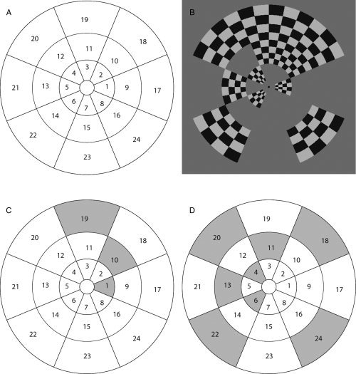
A: The 24 visual field regions examined in the present study. During the fMRI experiment each visual field region was stimulated with contrast‐reversing checkerboard pattern. In contrast to an earlier multifocal mapping study [Vanni et al., 2005], we reduced interactions between the neighboring visual areas [Pihlaja et al., 2008] by presenting the stimulus in two different sets of regions in two consecutive time intervals. This ensured the activation of V2 in visual field subareas for all participants. However, three subareas from the 432 total expected activations were not activated above the threshold. Within a set, only corner‐neighbors and no bordering neighbors were stimulated in one time interval. B: An example set of active regions (1, 4, 6, 10, 11, 13, 18, 19, 20, 22, 24) within one miniblock. This set was divided into two groups. C: The first set comprising regions (1, 10, 19) was on for 115 + 115 ms (opposite contrast), followed by 135 ms mid‐gray background. D: The second set of regions (4, 6, 11, 13, 18, 20, 22, 24) was presented correspondingly. The sequence was repeated four times within one miniblock (7.2 s). In other respects the multifocal design followed earlier work [Vanni et al., 2005]. The stimulated regions in the visual suppression task were the Sites 6 and 8, with the upper visual field control Sites 2 and 4.

The multifocal stimuli were presented with a three‐micromirror data projector (Christie X3^™, Christie Digital Systems Ltd., Mönchengladbach, Germany) using Presentation^™ software (Neurobehavioral Systems Inc., Albany, CA). Participants fixated on a point in the middle of a back‐projection display (mean luminance: 22 cd/m²) from 35 cm viewing distance. First four functional volumes were discarded to reach stable magnetization, followed by 32 blocks, with 7.3 s (4 volumes) duration each. During each block, each visual field region was inactive (uniform luminance of 22 cd/m2) or active, with a 4 × 4 checkerboard of 82% Weber contrast between the dark (4 cd/m²) and light (40 cd/m²) checks, contrast reversing at 8.3 Hz. Four runs were measured for each participant in one session. Each run comprised 132 volumes.

Measurements were carried out with a 3‐T MRI scanner (Signa^™ VH/I, General Electric Inc., WI) with a phased array 8‐channel coil. For functional imaging, the single shot gradient‐echo echo‐planar imaging sequence had parameters TR = 1800 ms, TE = 30 ms, matrix 64 × 64, flip angle 60°, FOV = 160 × 160, slice thickness 2.5 mm. At the end of the mapping session, high‐resolution anatomical images were acquired (matrix 256 × 256, FOV 250 × 250, slice thickness 0.9 mm).

All functional reconstructed data were first converted to Analyze‐format, and then processed with the SPM2 Matlab^™ (Mathworks Ltd., Natick, MA) toolbox (by Wellcome Department of Imaging Neuroscience, London, UK). Standard slice timing and motion correction were applied. The general linear model was fitted with one regression component for each of the 24 regions, comprising a box‐car model of activation blocks convolved with the default SPM2 hemodynamic response function, plus a separate constant regressor for the mean signal for each of the four runs.

The SPM T‐maps were estimated as follows: Separately for each voxel, a temporal model of activation and nuisance terms was estimated from the data. The calculated T‐values were then written to an image volume. SPM T‐maps were visualized together with anatomical 3D image, and borders between the early visual areas were identified at the horizontal and vertical meridian representations of the 24 stimulated regions. When TMS pulses were directed by using the mffMRI‐guided stimulation approach, the visual field representations of the TMS stimulation sites were at the innermost ring diagonally (Regions 6 and 8), between the horizontal and vertical meridians (Figs. 1 and 2). The approximate centers of the selected subareas were visually determined in SPM and corresponding coordinates were later used as the stimulation target sites in eXimia NBS software.

Figure 2.

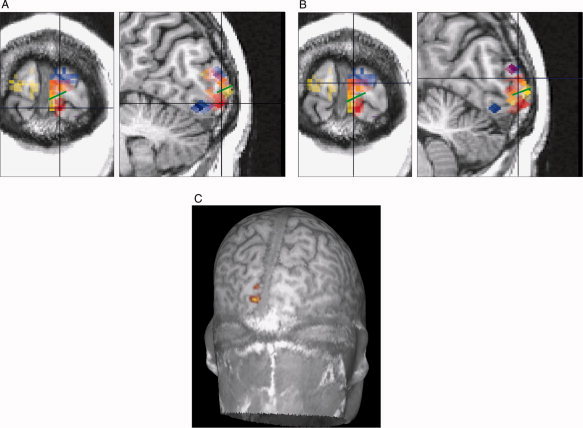
(A) and (B) show the corresponding subareas of V1 and V2 for visual field Regions 5 (blue), 6 (red), and 7 (yellow) in single participant data (P9). The crosshairs indicate subarea 6 in V1 (A) and V2 (B) and the green line the border between V1 and V2d. If two visual field regions activate the same cortical location it is shown with merged colors. Because of the depth and location differences, in this participant subarea 6 for V1 and V2 is best comparable in the coronal view. C: An MRI peeled at 17 mm depth showing the location of V1 and V2 subarea 8 in participant P8. The upper activation area is V2 and the lower one is V1. [Color figure can be viewed in the online issue, which is available at wileyonlinelibrary.com.]

Transcranial Magnetic Stimulation

Magnetic stimulation

TMS pulses were delivered by the eXimia TMS magnetic stimulator (Nexstim Ltd.) equipped with a figure‐of‐eight Nexstim bipulse coil (outer winding diameter = 70 mm; pulse length 280 μsec) which delivers the biphasic pulse with peak B field of 2 T at 100% of stimulator output at 2.5 mm distance from the coil plane. During the stimulation the coil was held tight against the participant's head by using a coil holder, and the participant's head was propped up with a chin rest. Earplugs were used to attenuate the sound of the TMS pulse‐induced noise. The coil plane was oriented tangentially to the scalp. The relationship between the brain and the TMS coil was registered continuously by using an MRI‐guided navigated brain stimulation (NBS) system (eXimia 2.1.1; Nexstim Ltd.) with a 1.6 mm accuracy of the recorded coil location with respect to the head tracker and the head [see Ruohonen and Karhu,2010]. During visual suppression and phosphene threshold measurements, the coordinates of the coil location and the location and strength of the calculated maximal E‐field in the target brain depth (defined previously according to the location of the occipital target region) were monitored during each TMS pulse. During visual suppression and phosphene threshold experiments, the E‐field of the second phase of the biphasic pulse was directed horizontally from lateral to medial. This current direction has been shown to be optimal to induce scotomas [Corthout et al.,2001] and phosphenes [Kammer et al.,2007]. The focal area of the stimulation hotspot of the TMS‐induced E‐field (defined as 98% of the maximum stimulating E‐field, calculated 20 mm below the coil in spherical conductor model representing the human head) is about 0.68 cm² with the 5.7 mm specified system accuracy including all error sources of eXimia NBS (i.e., coil localization, movement of the head tracker during an examination, E‐field computational model, registration to anatomical MRIs) [see Ruohonen and Karhu,2010]. Thus, both sulci and gyri are likely to get affected by the same current direction regardless of whether the center of the target is located in the sulcus or in the gyrus.

Computational modeling of the TMS‐induced E‐field

The intracranial E‐field distribution was calculated and visualized on the participant's anatomical MRI images by the eXimia NBS system for each single TMS pulse. The E‐field calculation was based on the spherical conductor model (for the mathematical formulation, see Heller and van Hulsteyn [1992], Ilmoniemi et al. [1999] and Sarvas [1987]) in which the modeling of the induced E‐field in the tissue is based on the shape of the induction coil, the location and orientation of the coil with respect to the tissue and the electrical conductivity structure of the tissue [Ilmoniemi et al.,1999]. Thus, the E‐field computation in the eXimia NBS takes into account the shape of the copper spirals inside the TMS coil, the coil orientation and location, current direction and the overall shape of the head and the brain.

Hämäläinen and Sarvas [1989] compared neuromagnetic fields computed either with the spherical model or with a realistically shaped head model in magnetoencephalography (MEG) and found that since the shape of the head is almost spherical in the occipital area, the spherical model suits well for modeling the magnetic field in the occipital area, especially if the depth of the target site is up to 40 mm. Because of reciprocity between the electromagnetic theories for MEG and TMS, the spherical model is applicable for TMS [Ilmoniemi et al.,1999; Ruohonen and Ilmoniemi,1998; Ruohonen and Ilmoniemi,1999].

The spherical conductor model does not take into account the conductivity differences caused by individual gyral folding pattern. By using finite‐element modeling (FEM), Haueisen et al. [2002] studied the influence of anisotropy on the EEG and MEG and concluded that source strength estimation may depend on tissue conductivity. In particular, earlier FEM studies indicate that the E‐field is maximal in the head tissue regions where the conductivity is low and that the direction of the current in anisotropic tissue tends to be along the direction of the lowest conductivity [Cerri et al.1995; Ilmoniemi et al.1999; Wang and Eisenberg,1994]. However, radial asymmetric anisotropy does not have influence to the induced E‐field in the spherically symmetric conductor model [Ilmoniemi,1995]. These findings indicate that a more realistic model of conductor anisotropy might modify the E‐field strength estimates in the present study. Nevertheless, it was recently demonstrated by applying FEM that E‐field strength is increased when induced currents are perpendicular to the local gyrus orientation, but the effect is restricted to the gyral crowns [Thielscher et al.,2011]. While the sulcal banks were not affected in Thielscher et al. [2011], it is generally assumed that columnar structure in the sulcal banks is the primarily affected site of TMS stimulation, because cortical orientation in relation to the TMS‐induced E‐field is optimal in sulcal banks [Fox et al.,2004].

In conclusion, the spherical conductor model is satisfactory to explain the induced E‐field distribution if the target regions are close to the surface of the head [see also Davey,2008; Ruohonen and Karhu,2010; Tarkiainen et al.,2003]. In this study, the selected cortical areas that were targeted with TMS were within 25 mm from the surface of the head. Thus, the TMS‐induced E‐field calculation by using the spherical conductor model can be considered suitable for the experimental purposes of this study.

TMS coil location in visual suppression and phosphene threshold determination

The mffMRI experiment provided 24 retinotopic subareas for V1 and V2, from which we aimed to choose the optimal subarea for the TMS stimulation of V1 in the phosphene threshold determination and the visual suppression task. The selection criteria required that: (1) V1 subarea would be as close to the head surface as possible (<25 mm); (2) V1 and the retinotopically equivalent V2 subarea would be located as far from each other as possible. For five participants the selected subarea was in the left hemisphere (this subarea represents Region 8, see Fig. 1), and for four participants, it was in the right hemisphere (Region 6, see Fig. 1). The selected V1 subareas were located ∼ 16 mm in depth (SD, 3.0 mm; range, 12–19 mm) and V2d subareas were ∼ 12 mm deep (SD, 2.5 mm; range, 9–17 mm). The mean distance between the approximate centers of subareas V1 and V2d was 11 mm (SD, 2.6 mm; range, 8–14 mm).

Phosphene and suppression thresholds

To determine how strong the induced E‐field strength should be to produce a cognitive effect, either facilitatory or inhibitory, we assessed the induced E‐field strength that is required to induce phosphenes and the E‐field strength that is required to induce visual suppression. By having the information about the relationship between the strength of E‐field and the cognitive processes, we were able to evaluate whether the adjacent (not purposely targeted) areas were also unintentionally but sufficiently affected to modify the behavioral effect.

The phosphene threshold was defined as the pulse intensity that induces phosphenes with 50% probability [e.g., Deblieck et al.,2008; Kammer et al.,2001]. Participants, sitting in a chair in a dim room with the eyes closed, were instructed to report after each pulse whether they saw a phosphene or not. We asked the participants to focus their attention nearby the fovea because the TMS pulses were targeted in the subarea corresponding to the visual field region between 1° and 3.2° from fixation and it has been shown that spatial attention enhances the detectability of phosphenes [Bestmann et al.,2007]. Phosphene thresholds were determined for four participants by the maximum likelihood threshold hunting (MLTH) procedure [Awiszus,2003]. For five participants the MLTH procedure could not be used because they were not aware of phosphenes in the trials with high stimulator output intensity (150% of the phosphene threshold) (for similar findings, see Kastner et al. [1998]). The dropoff of phosphenes is most probably caused by muscle twitches that the stimulation induces with higher intensities which capture attention from momentary phosphenes. The phosphene threshold was defined for them by delivering pulses in a randomized order in steps of one percentage unit starting from 30% to ∼ 55% of the stimulator output intensity. The procedure was repeated until the phosphene threshold could be determined. The mean E‐field strength of the phosphene threshold at 15 mm distance from the coil plane was 100 V/m (with the mean 45% of the maximal stimulator output intensity).

In the visual suppression task, the mean E‐field strength was 120 V/m at 15 mm distance from the coil plane. The lowest stimulator output intensity for the visual suppression (i.e., 120% of the phosphene threshold) was determined in the pilot studies (n = 3). The aim was to select as low an intensity as possible to induce the spatially most specific suppression effect. The criterion for a successful suppression required that the accuracy of the letter perception would be under 60% of the optimal performance at least in one of the nine SOAs (stimulus onset asynchronies). The experimental set up was similar to that in the main experiment (see below).

Stimuli and procedure in visual suppression task

During each session, participants sat in a dimly lit room. The visual stimuli were three dark gray letters (H, T, O) (diameter 0.23°), presented with Presentation^™ software on a gray background (31 cd/m²) in a CRT monitor at a 90 cm distance. In each trial, a fixation cross (diameter 0.25°) appeared for 1.5 s. It was followed by one of the letter stimuli for 16.5 ms in the upper or lower visual field region (2.8° away from fixation) and then again by the fixation cross until the participant had responded. The participants' task was to identify the letter stimulus, and they gave the forced‐choice response with the right hand. After each response, participants evaluated their subjective visual experience of the stimulus, but the results from these ratings will not be reported here.

For TMS stimulation, the multifocal subarea (the cortical area comprising representation for one of the 24 regions in the visual field, Fig. 1) 6 or 8 was selected individually for each participant on the basis of the relative locations of V1 and V2 in mffMRI data. If Subarea 6 was stimulated, then the letter stimulus was presented randomly either to the multifocal Region 6 in the lower left field or to Region 2 in the upper right field. Alternatively, if Subarea 8 was stimulated, then the letter stimulus was presented randomly either to the multifocal Region 8 in the lower right field or to Region 4 in the upper left field. In half of the trials the stimulus was presented to the lower, whereas in another half to the upper visual field. Thus, for each participant, the unstimulated upper field region served as a control site.

Prior to the actual experiment, the contrast level of the stimulus for each participant was set individually to reach 75–85% recognition accuracy by varying the luminance of the stimuli (mean luminance 6.4 cd/m²; range = 0.18–17.63; 99%–43% Weber contrasts between the background and the visual stimulus).

TMS pulses were delivered to V1 randomly at 9 different visual stimulus‐TMS‐onset asynchronies, ranging from 24 to 184 ms in steps of 20 ms (24 trials/visual field/SOA). The experiment was divided into eight TMS blocks (54 trials each). In addition, participants performed baseline blocks without TMS pulses (2 × 54 trials).

Localization of V1: The external anatomical landmark and mffMRI‐guided approaches

First, we explored the distribution of the E‐field in V1 and V2 for eight healthy adults (age, 21–28 years; two males) when the TMS coil was placed 2 cm above the inion (external anatomical landmark method). The coil plane was placed tangentially on the scalp and the current was directed horizontally for all participants. Participants did not carry out any psychophysical experiment, only TMS pulses were delivered at the individually defined intensity (120% of the participant's own phosphene threshold). After the TMS stimulation, E‐field strength in the centre of each of the 24 retinotopic subareas of the V1 and V2 was determined. The data were analyzed in three ways. First, the five most affected subareas were selected from each participant to evaluate the distribution of the E‐field between (1) occipital areas (V1 vs. V2 vs. V1/V2 border), (2) the hemispheres, (3) visual fields (the upper vs. the lower) and (4) the eccentricity (1‐3.2° vs. 3.2‐6.7°). Second, only the most affected V1 and V2 subareas were compared within each participant in order to find out for how many participants the induced E‐field strength was higher in V1 than in V2 or higher in V2 than in V1. When a visual stimulus is presented to a specific location in the visual field it may be relevant to compare V1 and V2 only in the corresponding retinotopic areas. Thus, third, we identified the V1 subarea with the maximal E‐field strength and compared it with the E‐field strength of the corresponding V2 subarea. Respectively, the most affected V2 subarea was compared with the corresponding V1 subarea.

To estimate the effect of angle variation between the affected sulci/gyri and E‐field direction, we defined the main direction of the affected part of the gyri or sulci (depending on whether the approximate center of the target region was located in the sulcus or in the gyrus) by manually drawing a line to it on the structural image [for a similar approach see Kammer et al.,2007; Thielscher et al.,2010]. The angle between the line and the horizontal current direction was measured for the five most affected subareas for each participant. It is noteworthy that we defined the orientation of the cortex only at one point. Because of the large size of subareas each subarea may have contained neurons oriented in other direction than it was defined here.

When the pulse was directed to V1 with mffMRI defined coil location during the visual suppression task (n = 9), we compared the E‐field strength in V1 with the E‐field strength of the unintentional stimulation of retinotopically equivalent V2d (Fig. 3A).

Figure 3.

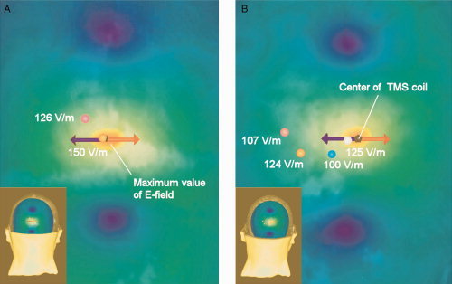
The distribution of the TMS‐induced E‐field at the visual suppression intensity (120% of the individual phosphene threshold) is illustrated for one participant (P7), when (A) the fMRI‐guided stimulation approach was applied and (B) when the external anatomical landmark approach was used. The colors orange‐yellow‐green‐blue indicate the strength of the E‐field in decreasing order. The red arrow illustrates the most effective current direction of the biphasic pulse and the blue arrow the less effective current direction. In (A) and (B), pink spot shows the approximate center of V2d Subarea 8 and orange spot represents the approximate center of V1 Subarea 8. The blue spot indicates the approximate center of V1 Subarea 6 and white spot the center of V2d Subarea 6. In (B), the E‐field strength is relatively high in V1 Subarea 8 even though the subarea seems to be located far from the E‐field hotspot. However, for this participant V1 Subarea 8 is located close to the skull surface, which explains the high E‐field. [Color figure can be viewed in the online issue, which is available at wileyonlinelibrary.com.]

RESULTS

Localization of V1 by Using the External Anatomical Landmark Method

The mffMRI experiment provided 24 cortical retinotopic subareas for V1 and V2, from which we aimed to define the most affected subareas (i.e., the subareas in which the induced E‐field strengths were the highest) when stimulation at the scotoma inducing intensity was directed 2 cm above the inion (n = 8). We selected the five most affected subareas for further analysis for each participant (40 subareas in total in the whole group). Compared to the most affected subarea (100%), the least affected subarea from the five most affected subareas received 69%–92% E‐field strength.

The E‐field distribution within the selected 40 subareas showed that on average V2 was the most activated area (Fig. 4A). The right hemisphere was affected more strongly than the left one. Further, 74% of the visual field regions corresponding to the most affected cortical subareas extended on the visual field between 1° and 3.2° and 26% of the visual field regions corresponding to the most affected subareas extended on the visual field between 3.2° and 6.7°. Only 5% of the most affected subareas represented the upper visual field.

Figure 4.

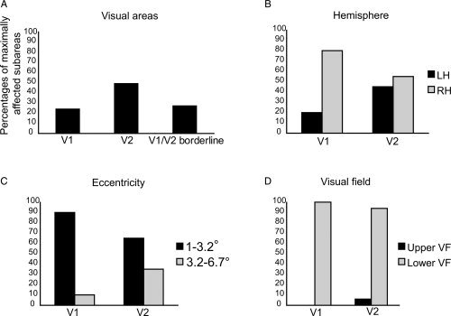
The distribution of the 40 most affected subareas when the position of the coil centre was 2 cm above the inion. The results are averaged from eight participants. A: More subareas with high E‐field were located in V2 than in other cortical areas. B: V1 showed stronger hemispheric asymmetry than V2, with more subareas with high E‐field distributed in the right hemisphere (RH) than in the left hemisphere (LH). C: The most affected regions were more often closer to the fixation in V1 than in V2. D: Almost always the strength of the E‐field was highest in the cortical representation of the lower visual field (VF).

Within V1, 80% of the most affected cortical subareas were in the right hemisphere, whereas in V2 the most affected subareas were located more equally in both hemispheres (Fig. 4B). The results also showed that the visual field region corresponding to the affected subarea in V1 was more often located between 1° and 3.2° from fixation than the region corresponding to the affected subarea in V2 (Fig. 4C). In addition, none of the visual field regions corresponding to the most affected five cortical subareas in V1 were located in the upper visual field (Fig. 4D).

The visualization of the data revealed that after delivering the pulse 2 cm above the inion, in most of the participants (7/8) the maximal E‐field hit the cortical representation of 1–3.2° eccentricity of either V1 or V2 (Fig. 3B). In one of the eight participants, the TMS pulse applied 2 cm above the inion landed outside the 24 identified subareas of V1 and V2. While most of the participants had minor (less than 10%) difference in the E‐field strength between V1 and V2, three participants showed more than 20% stronger E‐field over V2 than V1 subareas.

When the most affected V1 subarea was compared only with the retinotopically corresponding V2 subarea, the results still showed that the difference between the E‐field strengths was minor. Only for two participants the difference between V1 and V2 was more than 10%. With the external anatomical landmark method for seven participants out of eight the most affected subarea in V1 was the representation of Region 6. The comparison of the most affected V2 subarea and the retinotopically corresponding V1 showed that V2 had at least 20% higher E‐field strength than V1 for five participants. The most affected subareas for V2 were: region 2, 5, 6, 14, and 16.

We calculated the angle between the direction of the TMS‐induced E‐field and the main direction of the underlying gyrus/sulcus at the target area (i.e., at the point of the approximate center). About 20% of the approximate centers of the subareas were located exactly in the end of the curvature of the c‐shaped gyrus or sulcus (location in which the cortex is bending strongly), and the main course of the gyrus or sulcus was difficult to define due to more than one alternative. In these cases, two researchers evaluated the data independently and the mean of these two results was calculated. The mean angle between the direction of the induced current and the targeted gyri/sulci was 105° for V1 (SD 48°, min 31°, max 170°), 96° for V2 (SD 45°, min 4°, max 165°), and 103° for V1/V2 border (SD 34°, min 39° max 150°), showing that the variability in the orientation of the underlying gyri/sulci was similarly broad for all visual areas and therefore it was not likely to confound the results.

Localization of V1 by Using the mffMRI‐Guided Stimulation Approach

The TMS‐induced E‐field modeling provided estimates of the most affected cortical site when TMS pulses were directed to V1 during the visual suppression task (n = 9) with the help of individual mffMRI data (Fig. 3A). The E‐field strength at the phosphene threshold intensity was on average 17% lower than the E‐field strength that induced visual suppression. Assuming that the cortical excitability within early visual areas is uniform (see Murphey and Maunsell [2007] for comparison of phosphene thresholds in visual areas), it can be concluded that if the percentual difference between the E‐field strengths in V1 and V2d was higher than 17%, the subarea with lower E‐field strength did not induce the visual suppression but TMS had an effect on visual information processing in the subarea with higher E‐field.

On average, the selected V1 subareas were located 4 mm deeper than the selected V2d subareas (t(8) = 3.28, P < 0.05). The E‐field strength at the stimulator output intensity of 120% of the phosphene threshold at the target site V1 was highly variable between participants (see Fig. 5). V1 was more affected by TMS than V2d for four of the nine participants (mean difference between the E‐fields was 20.1%, see Fig. 5). For the remaining five participants, the E‐field was higher in V2d. For two of them, V2d received about 32% stronger activation than V1 and for three participants, the corresponding difference was less than 10%.

Figure 5.

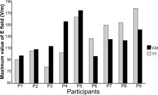
The distribution of the TMS‐induced E‐field in retinotopically corresponding visual field region representations of V1 and V2d, when individual mffMRI data was used to direct the TMS pulse to V1. For four participants out of nine the E‐field was stronger in V1 than in V2d.

The psychophysical data from all participants showed that the strongest suppression of the letter‐stimuli detection occurred consistently in the lower visual field (Fig. 6A). The significant interaction between the visual stimulus‐TMS‐onset asynchrony and the visual field (repeated measures ANOVA: F _[8,64] = 4.049; P < 0.025) revealed a decrease in letter‐detection accuracy occurring for the lower visual field stimuli at stimulus‐TMS SOAs of 64 ms (P < 0.01), 84 ms (P < 0.01), and 184 ms (P < 0.025) when compared with the 24 ms SOA, at which visual input has not yet reached the cortex when TMS is applied. The psychophysical performance in the control site (that is, the upper visual field region) was not affected at all by TMS stimulation even though the corresponding cortical subarea of the upper visual field region was located on average only 19 mm from the TMS‐targeted V1 subarea.

Figure 6.

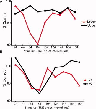
A: Average accuracy of letter‐recognition in nine participants when the TMS pulse was directed to the lower visual field representation in V1 with various stimulus‐TMS‐onset asynchronies. The visual stimuli were presented either to the lower (TMS targeted) or to the upper (control) visual field region. All results are compared with the baseline condition with no TMS so that 100% is the baseline. Letter‐recognition accuracy for upper visual field stimuli was not affected by TMS stimulation, whereas recognition accuracy for the lower visual field stimuli decreased at specific SOAs. B: The difference curves between the upper and lower visual field stimuli. The results of average accuracy of letter‐recognition in y‐axis were first compared with the baseline condition with no TMS. The red line represents the performance of the participants for whom the E‐field was higher in V1 (n = 4) and the black line represents the performance of the participants for whom the E‐field was higher in V2d (n = 5). [Color figure can be viewed in the online issue, which is available at wileyonlinelibrary.com.]

The location of the target V1 and V2d subareas at the cortex were highly variable between the participants. For three participants (P1, P4, and P9) the subarea V1, and for one participant (P9) also subarea V2d, was located mainly in the gyral crown in the mesial cortex. Because of the size of V1 and V2d subareas (diameter about 5–15 mm), the subareas frequently contained cortex aligned perpendicularly, diagonally and parallely to the E‐field, hindering reliable evaluation of anisotropy to the effective E‐field for example by using cortical column‐based cosine model [see Fox et al.,2004]. It is likely that cortical columns in various orientations in relation to E‐field were affected within subarea because of the size of the focal area of the TMS induced E‐field hotspot and the size of the specified system accuracy of eXimia NBS system. Nevertheless, for three participants the direction of the sulcus in relation to the E‐field was more obvious: for participant P2 V2d subarea was perpendicular to the E‐field. For participants P7 and P8 V1 subarea was aligned diagonally (about 45° angle) to the E‐field. For none of the participants the V1 or V2d subareas were located purely at the gyral crown or sulcal bank parallel to the scalp that would hinder the possibility of hitting the cortical columns, because both cortex and E‐field would be oriented parallely to each other.

DISCUSSION

This study aimed at answering two central questions relevant for TMS studies of visual cortex: (1) Is V1 more strongly affected than V2 when the traditional paradigm relying on the external anatomical landmark, 2 cm above the inion, is used to target V1? (2) Is it possible to selectively stimulate the representation of parafoveal visual field in the V1 by using one of the best available methodologies, namely individual retinotopic mffMRI maps of V1 and V2, coupled with brain navigation and TMS‐induced E‐field modeling?

As to the question (1), the TMS‐induced E‐field distribution showed that the standard stimulation site of 2 cm above the inion affected V2 more strongly than V1. However, we found also considerable interindividual variation in the sites that were most affected. For some participants, V1 was much less affected than V2, whereas for five of the eight participants the differences in the strength of the induced E‐fields were minor between V1 and V2. These main results are consistent with the previous findings [Okamoto et al.,2004; Steinmetz et al.,1989; Towle et al.,1993] showing that the standard occipital landmarks of the international 10–20 system exhibit great individual variation with respect to the individual brain anatomy. Moreover, our results showed that 90% of the subareas with the highest induced E‐field in V1 were within 1–3.2° from fixation, while the percentage was remarkably lower in V2 (65%). These results are in line with Kastner et al. [1998] who argued, based on their behavioural data, that the scotomas at 1–3° are probably due to the stimulation of V1, V2, and V3, whereas scotomas at eccentricities 4‐7° are due to the stimulation of V2 and V3 but not of V1.

When mffMRI was applied to direct TMS pulses to V1, the E‐field was notably stronger in V1 than in V2d for about half of the participants. Thus, retinotopic maps helped to target the V1, but at the group level selective stimulation of V1 was nevertheless unachievable. Thielscher et al. [2010, p. 329] suggested that “a specific targeting of V1 seems hardly to be possible, as for the subjects tested, there was no coil position and no position of the visual stimulus that would yield stronger electric fields in V1d than V2d”. We do not entirely agree with this conclusion. Our results show that selective V1 stimulation is possible in some of the participants but impossible in others, depending on the details of individual functional anatomy. There are notable differences between our and Thielscher et al.'s study. First of all, Thielscher et al. stimulated the visual field closer to the fovea (eccentricity from 0.45° to 0.9°) than we did in the present study. This may have made the selective stimulation of V1 even more difficult. Furthermore in our study, a larger number of possible stimulation sites for each participant were explored than in Thielscher et al.'s study, because we defined 24 retinotopic subareas from V1 and V2 in the two hemispheres and systematically aimed to search for the optimal V1 stimulation site whereas Thielscher et al. [2010] defined dorsal V1, V2, and V3 in one hemisphere.

While the 3D coordinates extracted from mffMRI were insufficient to determine the most affected site in multiple functional areas (V1, V2, V3d, V3a), mffMRI proved to be a suitable method for determining the retinotopic TMS stimulation sites in the occipital lobe, as we found a spatially precise suppression of corresponding visual field stimuli. TMS‐induced visual suppression was present in time windows from 64 to 84 ms for both groups of participants (higher E‐field in V2d or in V1), which indicate that both V1 and V2d may be equally susceptible to the effects of TMS. Thus, in addition to an intact V1, also an intact functioning of V2d may be a prerequisite for the visual discrimination of letter stimuli. This finding is consistent with the earlier report that V2d and V3 might be the sites of TMS‐induced visual suppression [Thielscher et al.,2010]. Furthermore, our results indicate that there may be another late suppression effect in early visual cortex around 184 ms post stimulus in addition to the 64 to 84 ms dip. The visualization of the data (Fig. 6B) suggests that the late dip is stronger for the participants to whom the E‐field is higher in V1 than in V2d. However, these findings remain to be confirmed in future studies targeting the TMS pulse directly to V2d or V1 during visual perception tasks.

Corthout et al. [2002] reported visual suppression as early as 20 ms post stimulus after occipital TMS. This early suppression effect might be explained by disruption of the input from lateral geniculate nucleaus to V1 [Thielscher et al.,2010]. Thus, early suppression would occur only for those of the participants for whom V1 is sufficiently close to the scalp [Thielscher et al.,2010]. However, in this study, we did not find any suppression effect at the 24 ms SOA, not even for the subgroup of participants who had a higher E‐field in V1 than in V2d. Thus, these results suggest that the 20 ms dip observed by Corthout et al. [2002] might have been a nonspecific effect of TMS.

So far, only very few studies investigated the cellular level neurophysiological mechanisms of TMS‐induced visual suppression and phosphenes. Historically, it has been established that a nerve is more excitable by longitudinal than transverse currents [Rushton,1927] and that the orthodromic current is the most effective [for review see Ranck,1975; Rushton,1927; Tranchina and Nicholson,1986]. In motor cortex stimulation, the optimal orientation of the TMS‐induced E‐field with respect to the central sulcus is along the cortical columns [Fox et al.,2004]. As to the studies concerning the visual cortex, Kammer et al. [2007] reported a nonsignificant trend which indicated that the phosphene thresholds were higher when the current was directed parallel to the course of the underlying gyrus. Thus, we can not rule out the possibility that if had we tried to direct the current perpendicular to the average direction of the sulcus in the mffMRI guided approach, the selectivity of V1 stimulation might have been improved. In the external anatomical landmark approach, we controlled the possibility that our results were systematically distorted by orientations of gyri or sulci in V1 or V2 by determining the main orientation of the underlying sulci or gyri. The analysis indicated similarly broad variability in the orientations of the underlying gyri/sulci for all visual areas.

In future studies, to obtain more definite understanding of the neurophysiological mechanisms of TMS‐induced phosphenes and visual suppression, at least three different factors should be considered: (1) the distribution of the E‐field in the early visual areas, (2) behavioral effects that are specific to given retinotopic or functional area, and (3) the E‐field orientation in relation to the sulcal bank. However, it may be complicated to base the evaluation of the anisotropy of early visual cortex on phosphene or scotoma thresholds, because visual brain areas have a complex surface geometry, and both phosphenes [Lee et al.,2000; Murphey and Maunsell,2007] and scotomas are likely generated by stimulation of every early visual area. It is possible that when the orientation of the coil is changed, the most effective spot of the E‐field moves to a location where it is approximately perpendicular to the sulcus. Thus, the perceptual threshold would not change with different coil orientation.

Finally, while the results demonstrate that functional and anatomical MR data without a mathematical model that defines the strength of the E‐field in different brain regions does not ensure selective V1 stimulation, the selective V1 stimulation can be achieved in a subset of participants by combining mffMRI with TMS‐induced E‐field modeling. Depending on the experimental task, the E‐field modeling could be applied to all multifocal subareas of V1 and V2 to find the optimal stimulation subarea for each individual and then to stimulate that site during visual tasks. Otherwise, without controlling for the stimulation site, one cannot make conclusions about the role of particular early visual areas. Consequently, these results and the study by Thielscher et al. [2010] have important implications for the interpretation of previous TMS studies that aimed to stimulate V1: Interindividual anatomical differences in the loci of early visual areas might contribute to the variable results in phosphene and scotoma studies.

CONCLUSION

Reliance on purely external anatomical landmarks is not sufficient in TMS studies if the aim is to determine the functional role of a particular visual area. If the TMS pulse is delivered 2 cm above the inion, the most affected area is most likely to be V2.

Although the selective stimulation of V1 appears difficult to achieve at the group level, it seems to be possible in at least some individual cases. In a subset of participants, when the anatomical MR navigation of TMS is combined with the functional mapping of retinotopic representation and with a model of the TMS‐induced E‐field in the cortex, selected V1 and V2d representations can be the primary target of stimulation and the activation distribution between functional areas can be modelled with sufficient accuracy. This way, the TMS‐induced disturbance can be located in a selective manner and the specific cognitive roles of the early visual areas can be tested in human participants. Future studies should address whether the selectivity of V1 stimulation could be increased even more by adjusting the coil orientation according to sulcal orientation of the target site.

REFERENCES

- Amassian VE, Cracco RQ, Maccabee PJ, Cracco JB, Rudell A, Eberle L ( 1989): Suppression of visual perception by magnetic coil stimulation of human occipital cortex. Electroencephalogr Clin Neurophysiol 74: 458–462. [DOI] [PubMed] [Google Scholar]
- Amunts K, Malikovic A, Mohlberg H, Schormann T, Zilles K ( 2000): Brodmann's areas 17 and 18 brought into stereotaxic space—Where and how variable? Neuroimage 11: 66–84. [DOI] [PubMed] [Google Scholar]
- Awiszus F ( 2003): TMS and threshold hunting. Suppl Clin Neurophysiol 56: 13–23. [DOI] [PubMed] [Google Scholar]
- Beckers G, Zeki S ( 1995): The consequences of inactivating areas V1 and V5 on visual motion perception. Brain 118: 49–60. [DOI] [PubMed] [Google Scholar]
- Bestmann S, Ruff CC, Blakemore C, Driver J, Thilo KV ( 2007): Spatial attention changes excitability of human visual cortex to direct stimulation. Curr Biol 17: 134–139. [DOI] [PMC free article] [PubMed] [Google Scholar]
- Boyer JL, Harrison S, Ro T ( 2005): Unconscious processing of orientation and color without primary visual cortex. Proc Natl Acad Sci USA 102: 16875–16879. [DOI] [PMC free article] [PubMed] [Google Scholar]
- Cerri G, De Leo R, Moglie F, Schiavoni A ( 1995): An accurate 3‐D model for magnetic stimulation of the brain cortex. J Med Eng Technol 19: 7–16. [DOI] [PubMed] [Google Scholar]
- Corthout E, Barker AT, Cowey A ( 2001): Transcranial magnetic stimulation—Which part of the current waveform causes the stimulation? Exp Brain Res 141: 128–132. [DOI] [PubMed] [Google Scholar]
- Corthout E, Hallett M, Cowey A ( 2002): Early visual cortical processing suggested by transcranial magnetic stimulation. Neuroreport 13: 1163–1166. [DOI] [PubMed] [Google Scholar]
- Corthout E, Hallett M, Cowey A ( 2003): Interference with vision by TMS over the occipital pole: A fourth period. Neuroreport 14: 651–655. [DOI] [PubMed] [Google Scholar]
- Corthout E, Uttl B, Juan, CH , Hallett M, Cowey A ( 2000): Suppression of vision by transcranial magnetic stimulation: a third mechanism. Neuroreport 11: 2345–2349. [DOI] [PubMed] [Google Scholar]
- Corthout E, Uttl B, Walsh V, Hallett M, Cowey A ( 1999a): Timing of activity in early visual cortex as revealed by transcranial magnetic stimulation. Neuroreport 10: 2631–2634. [DOI] [PubMed] [Google Scholar]
- Corthout E, Uttl B, Ziemann U, Cowey A, Hallett M ( 1999b): Two periods of processing in the (circum) striate visual cortex as revealed by transcranial magnetic stimulation. Neuropsychologia 37: 137–145. [DOI] [PubMed] [Google Scholar]
- Cowey A, Walsh V ( 2000): Magnetically induced phosphenes in sighted, blind and blindsighted observers. Neuroreport 11: 3269–3273. [DOI] [PubMed] [Google Scholar]
- Davey K ( 2008): Magnetic field stimulation: The brain as a conductor In: Wasserman EM, Epstein CM, Ziemann U, Walsh V, Paus T, Lisanby SH, editors. The Oxford Handbook of Transcranial Stimulation. New York: Oxford University Press; pp 33–46. [Google Scholar]
- Deblieck C, Thompson B, Iacoboni M, Wu AD ( 2008): Correlation between motor and phosphene thresholds: A transcranial magnetic stimulation study. Hum Brain Mapp 29: 662–670. [DOI] [PMC free article] [PubMed] [Google Scholar]
- Epstein CM, Zangaladze A ( 1996): Magnetic coil suppression of extrafoveal visual perception using disappearance targets. J Clin Neurophysiol 13: 242–246. [DOI] [PubMed] [Google Scholar]
- Fernandez E, Alfaro A, Tormos JM, Climent R, Martinez M, Vilanova H, Walsh V, Pascual‐Leone A ( 2002): Mapping of the human visual cortex using image‐guided transcranial magnetic stimulation. Brain Res Protoc 10: 115–124. [DOI] [PubMed] [Google Scholar]
- Fox PT, Narayana S, Tandon N, Sandoval H, Fox SP, Kochunov P, Lancaster JL ( 2004): Column‐based model of E‐field excitation of cerebral cortex. Hum Brain Mapp 22: 1–16. [DOI] [PMC free article] [PubMed] [Google Scholar]
- Hämäläinen MS, Sarvas J ( 1989): Realistic conductivity geometry model of the human head for interpretation of neuromagnetic data. IEEE Trans Biomed Eng 36: 165–171. [DOI] [PubMed] [Google Scholar]
- Haueisen J, Tuch DS, Ramon C, Schimpf PH, Wedeen VJ, George JS, Belliveau JW ( 2002): The influence of brain tissue anisotropy on human EEG and MEG. Neuroimage 15: 159–166. [DOI] [PubMed] [Google Scholar]
- Heinen K, Jolij J, Lamme VAF ( 2005): Figure‐ground segregation requires two distinct periods of activity in V1: A transcranial magnetic stimulation study. Neuroreport 16: 1483–1487. [DOI] [PubMed] [Google Scholar]
- Heller L, van Hulsteyn DB ( 1992): Brain stimulation using electromagnetic sources: Theoretical aspects. Biophys J 63: 129–138. [DOI] [PMC free article] [PubMed] [Google Scholar]
- Ilmoniemi RJ ( 1995): Radial anisotropy added to a spherically symmetric conductor does not affect the external magnetic field due to internal sources. Europhys Lett 30: 313–316. [Google Scholar]
- Ilmoniemi RJ, Ruohonen J, Karhu J ( 1999): Transcranial magnetic stimulation—A new tool for functional imaging of the brain. Crit Rev Biomed Eng 27: 241–284. [PubMed] [Google Scholar]
- Jasper HH ( 1958): The ten twenty electrode system of the International Federation. Electroencephalogr Clin Neurophysiol 10: 371–375. [PubMed] [Google Scholar]
- Juan CH, Walsh V ( 2003): Feedback to V1: A reverse hierarchy in vision. Exp Brain Res 150: 259–263. [DOI] [PubMed] [Google Scholar]
- Kammer T, Beck S, Erb M, Grodd W ( 2001): The influence of current direction on phosphene thresholds evoked by transcranial magnetic stimulation. Clin Neurophysiol 112: 2015–2021. [DOI] [PubMed] [Google Scholar]
- Kammer T, Puls K, Erb M, Grodd W ( 2005a): Transcranial magnetic stimulation in the visual system. II. Characterization of induced phosphenes and scotomas. Exp Brain Res 160: 129–140. [DOI] [PubMed] [Google Scholar]
- Kammer T, Puls K, Strasburger H, Hill NJ, Wichmann FA ( 2005b): Transcranial magnetic stimulation in the visual system. I. The psychophysics of visual suppression. Exp Brain Res 160: 118–128. [DOI] [PubMed] [Google Scholar]
- Kammer T, Vorwerg M, Herrnberger B ( 2007): Anisotropy in the visual cortex investigated by neuronavigated transcranial magnetic stimulation. Neuroimage 36: 313–321. [DOI] [PubMed] [Google Scholar]
- Kastner S, Demmer I, Ziemann U ( 1998): Transient visual field defects induced by transcranial magnetic stimulation over human occipital pole. Exp Brain Res 118: 19–26. [DOI] [PubMed] [Google Scholar]
- Koivisto M, Railo H, Salminen‐Vaparanta, N (in press). Transcranial magnetic stimulation of early visual cortex interferes with subjective visual awareness and objective forced‐choice performance. Conscious Cogn. [DOI] [PubMed] [Google Scholar]
- Kosslyn SM, Pascual‐Leone A, Felician O, Camposano S, Keenan JP, Thompson WL, Ganis G, Sukel KE, Alpert NM ( 1999): The role of area 17 in visual imagery: Convergent evidence from PET and rTMS. Science 284: 167–170. [DOI] [PubMed] [Google Scholar]
- Laycock R, Crewther DP, Fitzgerald PB, Crewther SG ( 2007): Evidence for fast signals and later processing in human V1/V2 and V5/MT+: A TMS study of motion perception. J Neurophysiol 98: 1253–1262. [DOI] [PubMed] [Google Scholar]
- Lee HW, Hong SB, Seo DW, Tae WS, Hong SC ( 2000): Mapping of functional organization in human visual cortex: Electrical cortical stimulation. Neurology 54: 849–854. [DOI] [PubMed] [Google Scholar]
- Marg E, Rudiak D ( 1994): Phosphenes induced by magnetic stimulation over the occipital brain: Description and probable site of stimulation. Optometry Vision Sci 71: 301–311. [DOI] [PubMed] [Google Scholar]
- Meyer BU, Diehl R, Steinmetz H, Britton TC, Benecke R ( 1991): Magnetic stimuli applied over motor and visual cortex: Influence of coil position and field polarity on motor responses, phosphenes, and eye movements. Electroencephalogr Clin Neurophysiol Suppl 43: 121–134. [PubMed] [Google Scholar]
- Miller MB, Fendrich R, Eliassen JC, Demirel S, Gazzaniga MS ( 1996): Transcranial magnetic stimulation: Delays in visual suppression due to luminance changes. Neuroreport 7: 1740–1744. [PubMed] [Google Scholar]
- Murphey DK, Maunsell JHR ( 2007): Behavioral detection of electrical microstimulation in different cortical visual areas. Curr Biol 17: 862–867. [DOI] [PMC free article] [PubMed] [Google Scholar]
- Okamoto M, Dan H, Sakamoto K, Takeo K, Shimizu K, Kohno S, Oda I, Isobe S, Suzuki T, Kohyama K, Dan I ( 2004): Three‐dimensional probabilistic anatomical cranio‐cerebral correlation via the international 10‐20 system oriented for transcranial functional brain mapping. Neuroimage 21: 99–111. [DOI] [PubMed] [Google Scholar]
- Pascual‐Leone A, Walsh V ( 2001): Fast backprojections from the motion to the primary visual area necessary for visual awareness. Science 292: 510–512. [DOI] [PubMed] [Google Scholar]
- Paulus W, Korinth S, Wischer S, Tergau F ( 1999): Differential inhibition of chromatic and achromatic perception by transcranial magnetic stimulation of the human visual cortex. Neuroreport 10: 1245–1248. [DOI] [PubMed] [Google Scholar]
- Pihlaja M, Henriksson L, James AC, Vanni S ( 2008): Quantitative multifocal fMRI shows active suppression in human V1. Hum Brain Mapp 29: 1001–1014. [DOI] [PMC free article] [PubMed] [Google Scholar]
- Potts GF, Gugino LD, Leventon ME, Grimson WEL, Kikinis R, Cote W, Alexander E, Anderson JE, Ettinger GJ, Aglio LS, Shenton ME ( 1998): Visual hemifield mapping using transcranial magnetic stimulation coregistered with cortical surfaces derived from magnetic resonance images. J Clin Neurophysiol 15: 344–350. [DOI] [PubMed] [Google Scholar]
- Ranck JB ( 1975): Which elements are excited in electrical stimulation of mammalian central nervous system: A review. Brain Res 98: 417–440. [DOI] [PubMed] [Google Scholar]
- Ray PG, Meador KJ, Epstein CM, Loring DW, Day LJ ( 1998): Magnetic stimulation of visual cortex: Factors influencing the perception of phosphenes. J Clin Neurophysiol 15: 351–357. [DOI] [PubMed] [Google Scholar]
- Ro T, Breitmeyer B, Burton P, Singhal NS, Lane, D ( 2003): Feedback contributions to visual awareness in human occipital cortex. Curr Biol 13: 1038–1041. [DOI] [PubMed] [Google Scholar]
- Ruohonen J, Ilmoniemi RJ ( 1998): Focusing and targeting of magnetic brain stimulation using multiple coils. Med Biol Eng Comput 36: 297–301. [DOI] [PubMed] [Google Scholar]
- Ruohonen J, Ilmoniemi RJ ( 1999): Modeling of the stimulating field generation in TMS. Electroencephalogr Clin Neurophysiol Suppl 51: 30–40. [PubMed] [Google Scholar]
- Ruohonen J, Karhu J ( 2010): Navigated transcranial magnetic stimulation. Clin Neurophysiol 40: 7–17. [DOI] [PubMed] [Google Scholar]
- Rushton WA ( 1927): The effect upon the threshold for nervous excitation of the length of nerve exposed, and the angle between current and nerve. J Physiol 63: 357–377. [DOI] [PMC free article] [PubMed] [Google Scholar]
- Sack AT, van der Mark S, Schuhmann T, Schwarzbach J, Goebel R ( 2009): Symbolic action priming relies on intact neural transmission along the retino‐geniculo‐striate pathway. Neuroimage 44: 284–293. [DOI] [PubMed] [Google Scholar]
- Sarvas J ( 1987): Basic mathematical and electromagnetic concepts of the biomagnetic inverse problem. Phys Med Biol 32: 11–22. [DOI] [PubMed] [Google Scholar]
- Silvanto J, Lavie N, Walsh V ( 2005): Double dissociation of V1 and V5/MT activity in visual awareness. Cereb Cortex 15: 1736–1741. [DOI] [PubMed] [Google Scholar]
- Steinmetz H, Fürst G, Meyer BU ( 1989): Craniocerebral topography within the international 10‐20 system. Electroencephalogr Clin Neurophysiol 72: 499–506. [DOI] [PubMed] [Google Scholar]
- Stensaas SS, Eddington DK, Dobelle WH ( 1974): The topography and variability of the primary visual cortex in man. J Neurosurg 40: 747–755. [DOI] [PubMed] [Google Scholar]
- Stewart LM, Walsh V, Rothwell JC ( 2001): Motor and phosphene thresholds: A transcranial magnetic stimulation correlation study. Neuropsychologia 39: 415–419. [DOI] [PubMed] [Google Scholar]
- Tarkiainen A, Liljeström M, Seppä M, Salmelin R ( 2003): The 3D topography of MEG source localization accuracy: Effects of conductor model and noise. Clin Neurophysiol 114: 1977–1992. [DOI] [PubMed] [Google Scholar]
- Thielscher A, Reichenbach A, Uğurbil K, Uludağ K ( 2010): The cortical site of visual suppression by transcranial magnetic stimulation. Cereb Cortex 20: 328–338. [DOI] [PMC free article] [PubMed] [Google Scholar]
- Thielscher A, Opitz A, Windhoff M ( 2011): Impact of the gyral geometry on the electric field induced by transcranial magnetic stimulation. Neuroimage 54: 234–243. [DOI] [PubMed] [Google Scholar]
- Tranchina D, Nicholson C ( 1986): A model for the polarization of neurons by extrinsically applied electric fields. Biophys J 50: 1139–1156. [DOI] [PMC free article] [PubMed] [Google Scholar]
- Towle VL, Bolaños J, Suarez D, Tan K, Grzeszczuk R, Levin DN, Cakmur R, Frank SA, Spire JP ( 1993): The spatial location of EEG electrodes: locating the best‐fitting sphere relative to cortical anatomy. Electroencephalogr Clin Neurophysiol 86: 1–6. [DOI] [PubMed] [Google Scholar]
- Vanni S, Henriksson L, James AC ( 2005): Multifocal fMRI mapping of visual cortical areas. Neuroimage 27: 95–105. [DOI] [PubMed] [Google Scholar]
- Wang W, Eisenberg SR ( 1994): A three‐dimensional finite element method for computing magnetically induced currents in tissues. IEEE Trans Magn 30: 5015–5023. [Google Scholar]