Identifying the default‐mode component in spatial IC analyses of patients with disorders of consciousness

Abstract

Objectives:Recent fMRI studies have shown that it is possible to reliably identify the default‐mode network (DMN) in the absence of any task, by resting‐state connectivity analyses in healthy volunteers. We here aimed to identify the DMN in the challenging patient population of disorders of consciousness encountered following coma. Experimental design: A spatial independent component analysis‐based methodology permitted DMN assessment, decomposing connectivity in all its different sources either neuronal or artifactual. Three different selection criteria were introduced assessing anticorrelation‐corrected connectivity with or without an automatic masking procedure and calculating connectivity scores encompassing both spatial and temporal properties. These three methods were validated on 10 healthy controls and applied to an independent group of 8 healthy controls and 11 severely brain‐damaged patients [locked‐in syndrome (n = 2), minimally conscious (n = 1), and vegetative state (n = 8)]. Principal observations: All vegetative patients showed fewer connections in the default‐mode areas, when compared with controls, contrary to locked‐in patients who showed near‐normal connectivity. In the minimally conscious‐state patient, only the two selection criteria considering both spatial and temporal properties were able to identify an intact right lateralized BOLD connectivity pattern, and metabolic PET data suggested its neuronal origin. Conclusions: When assessing resting‐state connectivity in patients with disorders of consciousness, it is important to use a methodology excluding non‐neuronal contributions caused by head motion, respiration, and heart rate artifacts encountered in all studied patients. Hum Brain Mapp, 2012. © 2011 Wiley Periodicals, Inc.

INTRODUCTION

Recent progress in fMRI studies on spontaneous brain activity has demonstrated activity patterns that emerge without any task or sensory stimulation, showing promise for the study of higher order associative network functionality [Biswal et al., 1995; Cordes et al., 2000; Damoiseaux et al., 2006; Fox and Raichle, 2007; Fox et al., 2005; Greicius et al., 2003; Lowe et al., 1998; Mitra et al., 1997; Nir et al., 2006; Vincent et al., 2007; Xiong et al., 1999; Yang et al., 2007]. One of the most intensely studied resting‐state networks is the default‐mode network (DMN), which encompasses the precuneus/posterior cingulate (pC), mesiofrontal anterior/ventral and posterior parietal cortices [for review, see Fox and Raichle, 2007]. This physiological “baseline” of the human brain has been suggested to be related to internally oriented content [Vanhaudenuhuyse & Demertzi et al., 2011], self‐referential, or social cognition [Schilbach et al., 2008] and has been referred to as the “intrinsic network” [Fox et al., 2005; Golland et al., 2007]. Interestingly, the “default” network can be shown to anticorrelate with an “extrinsic network” [Fox et al., 2005; Golland et al., 2008] considered to be important in externally oriented tasks [Golland et al., 2007]. The potential clinical interest of fMRI studies of DMN connectivity is currently being assessed in different pathologies such as depression [Anand et al., 2005], schizophrenia [Calhoun et al., 2009], autism [Kennedy et al., 2006], multiple sclerosis [Lowe et al., 2002], dementia [Greicius et al., 2004; Rombouts et al., 2009], brain death [see case studies by Boly et al., 2009], and disorders of consciousness [Vanhaudenhuyse & Noirhomme et al., 2010]. There are two main ways to analyze resting‐state functional connectivity MRI (rs‐fcMRI): (1) hypothesis‐driven seed‐voxel [Fox et al., 2005] and (2) data‐driven independent component analysis (ICA) approaches [Kiviniemi et al., 2003; McKeown et al., 1998]—each offering their own advantages and limitations [Cole et al., 2010].

The seed‐voxel approach consists in extracting the BOLD time course from a region of interest (ROI) and determines the temporal correlation between this signal (seed) and the time course from all other brain voxels [Fox et al., 2005]. To better visualize the correlation pattern and better analyze its properties, the seed approach can be integrated with graph‐theory methods [e.g., Fair et al., 2008; Hagmann et al., 2008]. In rs‐fcMRI graph representations, the resting‐state BOLD time series for each of the ROIs extracted from the DMN are correlated among each other giving a correlation matrix, which can be represented as a weighted graph. To reduce spurious variance unlikely to reflect neuronal activity, the BOLD signal is preprocessed by temporal bandpass filter and spatial smoothing, by regressing out head motion curves, whole brain signal as well as ventricular and white matter signal, and each of their first‐order derivative terms [Fox et al., 2005]. This straightforward method has been widely adopted and offers consistent results [Fox and Raichle, 2007]. However, it has raised some discussion mostly related to the preprocessing procedure, especially concerning the regressing out of the global activity from the BOLD signal, which might induce some spurious anticorrelations [Fox et al., 2009; Murphy et al., 2009], and the selection itself of the seed regions, which is biased by a priori definition.

Contrary to the previous approach, ICA‐based rs‐fcMRI analysis [Kiviniemi et al., 2003; McKeown et al., 1998] does not require any a priori definition of seed regions. It analyzes the entire BOLD dataset and decomposes it into components that are maximally statistically independent [Hyvarinen et al., 2001]. A number of studies have shown that ICA is a powerful mathematical tool, which can simultaneously extract a variety of different coherent neuronal networks [De Luca et al., 2006; Esposito et al., 2008; Greicius and Menon, 2004; Greicius et al., 2003, 2004; McKeown et al., 1998] and separate them from other signal modulations such as those induced by head motion or physiological confounds [e.g., cardiac pulsation, respiratory cycle, and slow changes in the depth and rate of breathing, Birn et al., 2008; Perlbarg and Marrelec, 2008; Perlbarg et al., 2007]. However, ICA does not provide any classification or ordering of the independent components (ICs), and it is usually left to the user to decide which IC corresponds to the DMN. Automatic approaches have been proposed to remove user bias in selecting the component. For example the “goodness of fit” is based on matching with a previously built template [Greicius et al., 2004]. Self‐organizing ICA groups components from a group of subjects and the user (by visual inspection) selects the group that corresponds to the DMN [Esposito et al., 2005]. These approaches are based on the spatial extent of the component and some of them have been used in collaboration with a power spectrum analysis, removing all components with more than half of the power due to high frequencies [for the goodness of fit, see [Vanhaudenhuyse & Noirhomme et al., 2010]. Although having an automatic selection criteria based on spatial properties may be a big advantage when the network spatial pattern is still partially preserved, it may become a disadvantage for cases where the network is mostly destroyed. In these cases, only properly masking the regions of the brain where a preserved activity could be expected would help the selection but then other imaging techniques like, for example, PET should be used at the same time. The possibility instead to realize an automatic masking procedure, which will be only based on BOLD data, could then be an important solution for highly pathological cases. At the same time, giving more importance to time properties other than just the power spectrum like temporal entropy or one‐lag autocorrelation or to spatial properties no directly pattern‐related like, for example, spatial entropy could also be a valuable tool to improve the selection power.

The aim of this study is to assess resting‐state DMN connectivity in patients with severe brain damage such as the vegetative, minimally conscious, or locked‐in state, disentangling neuronal from artifactual sources. For the clinical use of these rs‐fcMRI measurements, we first validated an automated, user‐independent spatial ICA‐based procedure to select and analyze DMN functional integrity in healthy controls. This approach is based on both spatial and temporal information of the components. The temporal information and spatial properties other than the spatial pattern are given by the fingerprint of the component [De Martino et al., 2007]. Using more information enables a better characterization of artifactual correlations. Three different selection strategies were developed: (1) spatially pattern driven, (2) based on an automatic masking driven by the fingerprint properties (time domain dominated), and (3) based on a compromise between spatial and temporal properties. We next applied this methodology in an independent healthy control group and patients in locked‐in syndrome [i.e., pseudocoma; LIS, Laureys et al., 2004], minimally conscious state (i.e., showing fluctuating signs of awareness devoid of communication; MCS), or vegetative state (i.e., wakeful unawareness; VS). For the first selection criterion, which was only spatially pattern driven, we expected to perform equally well in healthy controls but more poorly than the other two in pathological brains.

MATERIALS AND METHODS

Subjects and MRI Acquisition

Three independent groups of healthy controls were analyzed for the full study. The first group (Group 1) was analyzed for the independent study on DMN ROIs selection (prior knowledge about the DMN equivalent to building a DMN spatial template) and for the creation of an average DMN fingerprint [De Martino, 2007]. The second group (Group 2) was analyzed to test the DMN selection criteria introduced in this manuscript and compare them with other available selection methods (validation of our methodology). The third group (Group 3) of healthy controls was introduced to compare rs‐fcMRI analyses results with respect to patients with disorders of consciousness. All subjects went through a resting‐state protocol in which they were instructed to keep their eyes closed and to remain awake.

Group 1 included 11 healthy volunteers with no neurological or psychiatric history (mean age = 71; SD = 6; range 62–80 years; nine women). Resting‐state BOLD data were acquired on a 3‐T MR scanner (Trio Tim, Siemens, Germany) with a gradient echo‐planar sequence using axial slice orientation (32 slices; voxel size = 3.44 × 3.44 × 3.9 mm³; matrix size = 64 × 64 × 32; repetition time = 2,130 ms, echo time = 40 ms, flip angle = 90°; field of view = 220 mm). A protocol of 250 scans lasting 533 s was performed. A T1‐weighted MPRAGE sequence was also acquired for registration with functional data on each subject.

Group 2 included 10 healthy volunteers with no neurological or psychiatric history (mean age = 21; SD = 3; range 18–28 years; four women). Resting‐state BOLD data were acquired on a 3‐T MR scanner (Trio Tim, Siemens, Germany) with a gradient echo‐planar sequence using axial slice orientation (32 slices; voxel size = 3.44 × 3.44 × 3.9 mm³; matrix size = 64 × 64 × 32; repetition time = 2,460 ms, echo time = 40 ms, flip angle = 90°; field of view = 220 mm). A protocol of 350 scans lasting 861 s was performed. A T1‐weighted MPRAGE sequence was also acquired for registration with functional data on each subject.

Group 3 included 8 healthy volunteers with no neurological or psychiatric history (mean age = 48; SD = 13; range 25–65 years; three women). Resting‐state BOLD data were acquired on a 3‐T MR scanner (Trio Tim, Siemens, Germany) with a gradient echo‐planar sequence using axial slice orientation (32 slices; voxel size = 3.0 × 3.0 × 3.75 mm³; matrix size = 64 × 64 × 32; repetition time = 2,000 ms, echo time = 30 ms, flip angle = 78°; field of view = 192 mm). A protocol of 300 scans lasting 600 s was performed. A T1‐weighted MPRAGE sequence was also acquired for registration with functional data on each subject.

Eight patients in VS (mean age = 61; SD = 30; range 16–87 years; all men), one MCS (age 24 years; male), and two LIS patients (aged 24 years; female and age 20 years; male) were studied with the same scanner used for the third group of healthy controls. Etiology of the VS was traumatic in three cases and nontraumatic in five cases; three patients were studied in the acute (i.e., <1 month postinjury) and five in the chronic setting. The MCS patient was traumatic, and the two LIS patients were studied 28 months postbasilar artery thrombosis and 4 years after trauma (see Table I for patients' demographic and clinical data). All patients underwent repeated behavioral evaluations by means of the Coma Recovery Scale Revised [Giacino et al., 2004] and the Glasgow‐Liège Scale [Born et al., 1985] performed by experienced clinicians (MB, AV, MAB, AD, and SL). The diagnosis was made according to internationally accepted criteria for VS [The Multi‐Society Task Force on PVS, 1994], MCS [Giacino et al., 2004], and LIS [American Congress of Rehabilitation Medicine, 1995].

Table I.

Patients' demographic, clinical, and structural imaging data

	VS1	VS2	VS3	VS4	VS5	VS6	VS7	VS8	MCS	LIS1	LIS2
Gender (age, years)	Male (62)	Male (21)	Male (16)	Female (69)	Male (82)	Male (87)	Male (38)	Male (63)	Male (24)	Female (24)	Male (20)
Etiology	Brainstem hemorrhage	Trauma	Trauma	Anoxia	Vascular encephalopathy	Trauma	Anoxia	Anoxia	Trauma	Brainstem stroke	Trauma
Time of fMRI (days after insult)	32	170	615	61	26	7	282	29	301	850	1,475
Outcome at 12 months	Dead	VS	VS	VS	Dead	Dead	VS	MCS	Still MCS	LIS	LIS
Auditory functiona	None	Startle reflex	Startle reflex	Startle reflex	None	None	Startle reflex	Startle reflex	Startle reflex	Consistent movement to command	Consistent movement to command
Visual functiona	Blink to threat	None	None	None	None	None	None	Blink to threat	Visual pursuit	Object recognition	Object recognition
Motor functiona	Flexion to pain	Abnormal posturing	Abnormal posturing	Flexion to pain	Flexion to pain	Flexion to pain	Abnormal posturing	Flexion to pain	Flexion to pain	Flexion to pain	Flexion to pain
Verbal/ Oromotor functiona	None	Oral reflexes	Vocalization	Oral reflexes	Oral reflexes	Oral reflexes	Oral reflexes	Vocalization	Oral reflexes	Oral Movement	Vocalization
Communicationa	None	None	None	None	None	None	None	None	None	Functional accurate	Functional accurate
Arousala	Without stimulation	Without stimulation	Without stimulation	With stimulation	With stimulation	With stimulation	With stimulation	Without stimulation	Without stimulation	Attention	Attention
EEG background activity	Diffuse theta‐delta,	Right‐lateralized theta‐delta, nonreactive	Irregular diffuse theta‐delta	Left lateralized diffuse theta‐delta	Symmetric theta‐delta, nonreactive	Irregular diffuse theta‐delta, nonreactive	Left‐lateralized theta, nonreactive	Diffuse theta‐delta, nonreactive	Not available	Diffuse theta, transient delta	Not available
Lesions on structural MRI	Pontine hemorrhage extending to midbrain	Diffuse axonal injury. Bilateral subdural frontal hygroma	Diffuse atrophy with secondary hydrocephalus. Bilateral lesions of lenticular nucleus thalamus, and parahippocampal structures	Diffuse bilateral white matter atrophy, caudate, thalamus, and parahippocampal lesions	Diffuse cortical and subcortical atrophy. Bilateral basal ganglia and white matter lesions	Subarachnoid hemorrhage, brainstem, left lenticular nucleus, temporal and multifocal frontoparietal contusions	Diffuse white matter lesions	Posterior occipitoparietal ischemia	Corpus callosum, left thalamus, pontine, bilateral frontoparietal lesions	Centro‐ protuberential lesion	Pontine, midbrain, cerebellum, left thalamus lesions

VS, vegetative state; LIS, locked‐in syndrome; MCS, minimally conscious state.

^aBased on Coma Recovery Score‐Revised assessment.

Written informed consent was obtained from all healthy volunteers and from the legal representative of all patients (and from the LIS patients using eye‐coded communication). The study was approved by the Ethics Committee of the Faculty of Medicine of the University of Liège, which complies with the Code of Ethics of the World Medical Association (Declaration of Helsinki).

Data Preprocessing and Analysis

fMRI data were preprocessed using the “BrainVoyager” software package (R. Goebel, Brain Innovation, Maastricht, The Netherlands). Preprocessing of functional scans included 3D motion correction, linear trend removal, slice scan time correction, and filtering out low frequencies of up to 0.005 Hz. The data were spatially smoothed with a Gaussian filter of full width at half maximum value of 8 mm. The functional images from each subject were aligned to the participant's own anatomical scan and warped into the standard anatomical space of Talairach and Tournoux [1988]. The Talairach transformation was performed in two steps. The first step consisted in rotating the 3D data set of each subject to be aligned with stereotaxic axes (for this step, the location of the anterior commissure (AC), the posterior commissure (PC), and two rotation parameters for midsagittal alignment was specified manually). In the second step, the extreme points of the cerebrum were specified. These points together with the AC and PC coordinates were then used to scale the 3D data sets into the dimensions of the standard brain of the Talairach and Tournoux [1988] atlas using a piecewise affine and continuous transformation. ICA [Formisano et al., 2004; Hyvarinen et al., 2001] was performed with the “BrainVoyager” software package using 30 components [Jafri et al., 2008; Koch et al., 2010; Meindl et al., 2010; Weissman‐Fogel et al., 2010; Ylipaavalniemi and Vigario, 2008]. A spatial mean was subtracted from all the voxels (mean calculated all over the voxels at a fixed time), and principal component analysis was applied for dimensionality reduction before performing ICA.

Decomposing Connectivity in Independent Component Graphs

We developed here a new methodology, which takes advantage of the capability of ICA, to decompose the signal in neuronal and artifactual sources but still preserves the concept of connectivity in a defined network of ROIs. This methodology in fact allows building for each IC a connectivity graph, which summarizes the level of connectivity for a defined network of ROIs according to the time behavior described by the correspondent IC time course. Our connectivity study used 13 ROIs defined on an average DMN map calculated on a group of 11 healthy subjects (Group 1). We performed, as implemented in Brain Voyager [self‐organizing ICA, Esposito et al., 2005], a spatial similarity test on single‐subjects ICs and we averaged the maps belonging to the cluster, which was selected by visual inspection as DMN. The selected 13 ROIs were the most representative regions of our average DMN map close to the DMN target points previously published [Fair et al., 2008; Fox et al., 2005] including: medial prefrontal cortex ventral (MFv) [−3, 39, −2], medial prefrontal cortex anterior (MFa) [2, 59, 16], pC [−3, −55, 21], left posterior parietal lobe (L‐pP) [−49, −60, 23], right posterior parietal lobe (R‐pP) [45, −61, 21], left superior frontal gyrus (L‐sF) [−19, 32, 51], right superior frontal gyrus (R‐sF) [23, 29, 51], left middle temporal gyrus anterior [−61, −11, −10], right middle temporal gyrus anterior [57, −11, −13], left parahippocampal/mesiotemporal [−23, −17, −17], right parahippocampal/mesiotemporal [25, −16, −15], left thalamus (L‐T) [−5, −11, 7], and right thalamus (R‐T) [4, −11, 6] (the ROIs were set initially to a cubic shape 10 × 10 × 10 mm³, and the center was chosen accordingly to the DMN extracted from Group 1, but once the ROI was saved in Brain Voyager only the ROI's voxels belonging to the DMN end up making the saved ROI).

To study connectivity between each pair of target points, we implemented a new method, which is based on ICA followed by a general linear model (GLM). After running ICA with 30 components, we used the corresponding time courses to regress in the BOLD signal in each of the 13 ROIs. The time courses from each ROI were extracted as the arithmetic mean of the time courses of the voxels belonging to the same ROI. Note that by using a smoothing of a 8‐mm kernel implies that taking an arithmetic mean as implemented in Brain Voyager or extracting the first eigenvariate will give similar results. For each component, we obtained 13 parameter estimates (beta values) indicating the weight of each regressor and the corresponding T‐values (see Appendix). To build a connectivity graph, we drew an edge between each pair of target points with T > Tth with Tth corresponding to 1 − P/78 for P = 0.05 with 267 degrees of freedom (Bonferroni correction for multiple comparisons was performed dividing P by the number of possible edges between the 13 nodes; 13*(13 − 1)/2 = 78). To account for the fact that ICA does not predict the sign of the ICs, the condition T < −Tth was also used. This allowed us to end up with two connectivity graphs for each of the 30 components (1–30 for the condition T > Tth and 31–60 for T < −Tth). We hypothesized that the number of edges E for each of the 60 connectivity graphs should be the highest for the component of the DMN. However, given that no regressing out of the global signal was applied, we did not pick the component corresponding to the graph with the largest number of total edges (i.e., the global component could appear as the main source of connectivity). Therefore, we implemented “anticorrelation‐corrected number of edges” (see Fig. 1). The anticorrelation‐corrected number of edges was obtained by multiplying the total number of edges of each graph by a weight “w,” which measures the anticorrelation of the DMN activity with the extrinsic system/external control network (ECN). Similarly to the 13 targets ROIs of the DMN, we selected as ROIs the five most representative regions of the extrinsic system appearing as anticorrelated regions in the DMN average map calculated on the Group 1 of healthy subjects close to the ECN target points previously published (Fox et al., 2005] including: (left supramarginal gyrus [−56, −33, 37], right supramarginal gyrus [54, −39, 38], left middle temporal gyrus posterior [−52, −53, −5], right middle temporal gyrus posterior [52, −57, −5], and supplementary motor area [2, 5, 46]). The anticorrelation‐corrected number of edges E _AntiCC was then defined in terms of the number of edges E as E _AntiCC = E*w (see Appendix), with the anticorrelation index w a number between 0 and 1. The index would be close to 0 if the activity in the extrinsic network highly correlates with the activity in the intrinsic network, e.g., a global signal, and close to 1 if the activity in the extrinsic network is anticorrelated with the activity in the DMN, e.g., the DMN component. A new number of edges could be built by just inverting the ± signs in the definition of E _AntiCC (see Appendix) obtaining a new number, which we called “global edges” and which is highest for the global component (see Fig. 1). This allowed us to isolate the global mode and to remove it from the full set of components.

Figure 1.

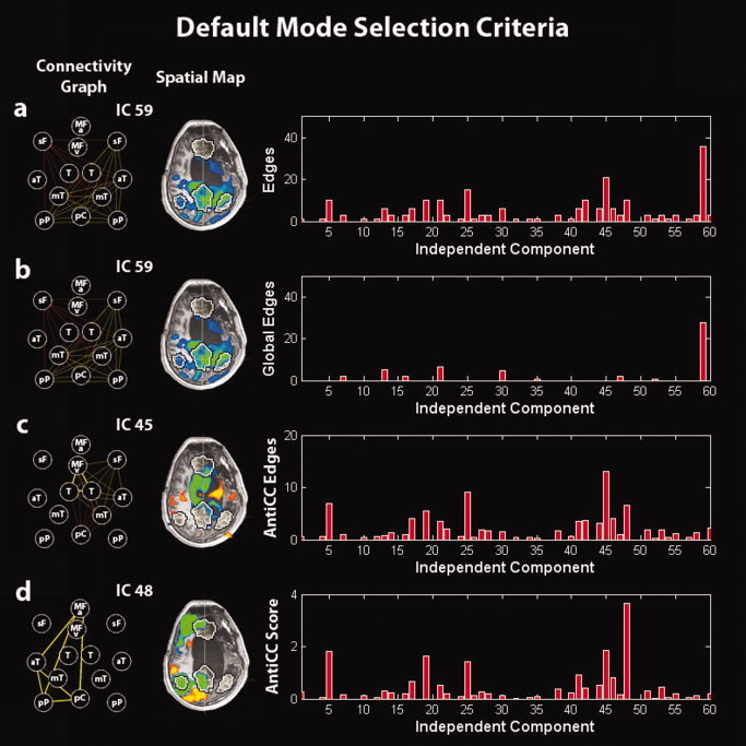
Illustration of the default‐mode selection method in a minimally conscious‐state patient. (a) Selection of the IC corresponding to the graph with the highest number of edges. (b) Selection of the IC corresponding to the graph with the highest number of global edges (to select the global signal IC). (c) Selection of the IC corresponding to the graph with the highest number of anticorrelation‐corrected edges. (d) Selection of the IC corresponding to the graph with the highest anticorrelation‐corrected score. Right panel: (a) number of edges, (b) number of global edges, (c) number of anticorrelation‐corrected edges, and (d) anticorrelation‐corrected score of each graph vs. the corresponding IC number. Middle panel: Spatial map of the selected IC. Left panel: Connectivity graph of the selected IC. MFv, medial prefrontal cortex ventral; MFa, medial prefrontal cortex anterior; pC, posterior cingulate/precuneus; pP, posterior parietal lobe; sF, superior frontal gyrus; aT, middle temporal gyrus anterior; mT, parahippocampal/mesiotemporal; T, thalamus. Left is right side of brain.

Selection Criteria

Three different strategies were developed: (1) spatially pattern driven, (2) based on an automatic masking driven by the fingerprint properties (time domain dominated), and (3) based on a compromise between spatial and temporal properties.

First selection criterion

This selection criterion selects as the DMN the component with the highest number of anticorrelation‐corrected edges (see Fig. 1). The number of anticorrelation‐corrected edges of the component selected is indicated in Tables I and II of the Supporting Information with the name “E _AntiCC init.”

Second selection criterion

This selection criterion is still based on the highest number of edges but after performing an automatic masking obtained by removing subsequently ROIs from the network (see flow chart in Fig. 2 and Appendix for the definition of the distance D _IC). The automatic masking proceeded by removing subsequently (going through all the 13 ROIs) one ROI (first step), then two regions together (second step), and three regions up to five regions (last step). At each step, the component selected as the one with the highest number of anticorrelation‐corrected edges in the reduced network and with the minimum distance among all the possible reduced networks (for that step) was tested by comparing its fingerprint (as in De Martino et al. [ 2007], the fingerprint reports normalized values, respectively, for: degree of clustering, skewness, kurtosis, spatial entropy as calculated from the distribution of the z values for the considered IC and one‐lag autocorrelation, temporal entropy, and the power of the five frequency bands [0–0.008, 0.008–0.02, 0.02–0.05, 0.05–0.1, and 0.1–0.25 Hz] as extracted from the time course of the considered IC) with an average fingerprint (distance D _IC from the reference fingerprint needed to be inside two standard deviations with the standard deviation calculated on each subject IC distances' distribution) built from the DMN components of the 11 healthy subjects (Group 1). The number of anticorrelation‐corrected edges of the component selected is indicated in Tables I and II Supporting Information with the name “E _AntiCC fin.”

Figure 2.

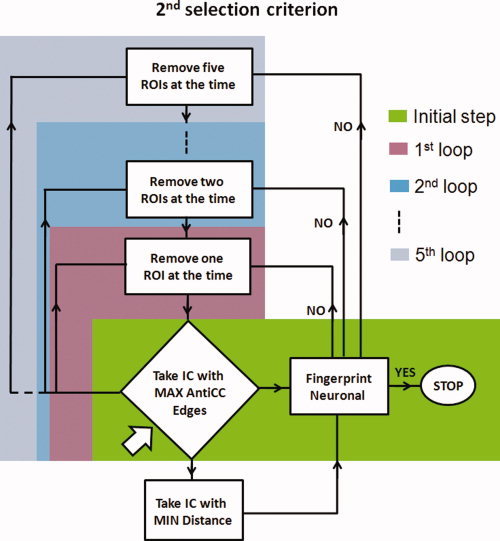
Flow chart illustrating the second selection criterion. Arrow indicates the starting point in the flow chart. Different color boxes indicate the different steps. [Color figure can be viewed in the online issue, which is available at wileyonlinelibrary.com.]

Third selection criterion

The third automatic selection criterion selects the component with the highest “anticorrelation‐corrected score” (S _AntiCC), built by multiplying the number of anticorrelation‐corrected edges by a new weight “w _F,” which measures the distance of its fingerprint from the average fingerprint of the DMN in healthy controls (Group 1). The weight w _F is close to 0 for components that have “artifactual” source and close to 1 for components with “neuronal” origin—the latter assumes that in healthy controls ICA was able to fully separate artifactual from neuronal sources. The number of anticorrelation‐corrected edges of the component selected is indicated in Tables I and II of the Supporting Information with the name “E _AntiCC (S _AntiCC max).”

The three selection criteria were compared with self‐organizing ICA, which selected for each single subject the most spatially similar component to a DMN average map based on the 11 healthy subjects of Group 1 (self‐organizing ICA used to cluster 30 average maps vs. 30 ICs maps).

Single‐Subject and Group Analysis

For each single subject, we presented a connectivity graph showing thin and thick lines in three colors: red, orange, and yellow. Thin and thick lines correspond, respectively, to the conditions T > Tth and T*w > Tth [thin line for edges and thick line for “weighted edges” (E _W)], and the three colors: red, orange, and yellow correspond, respectively, to P values P = 0.05, P = 0.01, and P = 0.001. It is important to note that the number of anticorrelation‐corrected edges, as previously stated, is calculated by the number of edges E (number of edges in the graph corresponding to the condition T > Tth for P = 0.05 multiplied by the corresponding anticorrelation index w) and is not obtained by counting the number of edges corresponding to the conditions T*w > Tth termed “weighted edges” (see Tables I and II in the Supporting Information to compare values).

Two‐tailed unequal variance Student's t‐test compared the total number of edges, the anticorrelation index, the anticorrelation‐corrected total number of edges, the total number of weighted edges, the anticorrelation‐corrected scores, and the ratio of the anticorrelation‐corrected score over the anticorrelation‐corrected total number of edges in the DMN in controls vs. VS patients for each of the three different selection criteria.

Spatial maps were obtained by running a two‐step analysis. First, the BOLD signal from each single subject was regressed with the time courses of the ICs selected as DMN as selected by the second selection criterion (automatic masking). Second, the estimated parametric maps entered a multisubject random‐effect analysis providing group‐level statistical T‐maps. Maps were thresholded at a false discovery rate corrected P < 0.05 within DMN mask obtained from an independent dataset (Group 1) shown as black and white contour volume of interest in Figures 3 and 5, 6, 7. The mean connectivity graph was derived by drawing an edge between each pair of ROIs with a sum of anticorrelation‐corrected beta values beta*w significantly different (permutation test) from the absolute value of their difference. Different colors correspond to differences in significance, with red, orange, and yellow representing P = 0.05, P = 0.01, and P = 0.001, respectively. Thicker lines are the connections that survive a multicomparison Bonferroni correction with the number of possible edges between the 13 nodes: 13*(13 − 1)/2 = 78.

Figure 3.

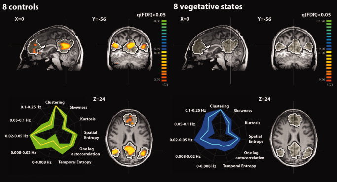
Upper part: Random‐effect group analyses identifying the default‐mode network (DMN) in eight healthy controls and eight patients in a vegetative state (VS). Results are thresholded at false discovery rate corrected P < 0.05 with a mask given by the black and white contour regions showing the DMN from an independent dataset (n = 11 healthy controls, Group 1). Lower part: Graphical representation (i.e., fingerprint; normalized values) of DMN temporal properties (five frequency bands, temporal entropy, and one‐lag autocorrelation) and spatial properties (spatial entropy, skewness, kurtosis, and clustering) in healthy controls [mean (yellow) and SD (green)] and in VS patients [mean (cyan) and SD (blue)]. [Color figure can be viewed in the online issue, which is available at wileyonlinelibrary.com.]

Figure 5.

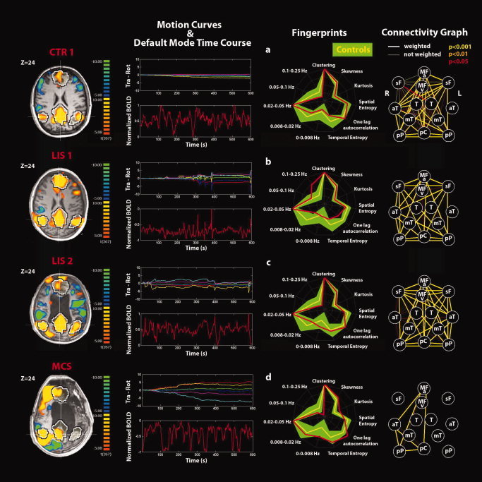
Single‐subject analyses identifying the default‐mode network (DMN) and connectivity graphs in (a) a representative healthy control, (b, c) LIS patients 1, 2, and (d) MCS patient. Positive correlations (yellow) and anticorrelations (blue) with the DM time course shown on a transverse section at Z = 24 mm (thresholded at corrected P < 0.05). Black and white contour regions show the DMN from an independent dataset of 11 healthy controls. Motion curves illustrate translation (in mm) for x (red), y (green), and z (blue) and rotation (in °) for pitch (yellow), roll (purple), and yaw (cyan) parameters, and the DMN time course illustrates the normalized BOLD signal over 600 s. The fingerprint summarizes the DMN temporal and spatial properties for each subject (red) superimposed to the control data of eight healthy subjects (mean in yellow and standard deviation in green). The connectivity graph illustrates the connections between the 13 selected DM nodes at different thresholds for significance (thick lines, “weighted edges” are corrected for external network anticorrelations). Nodes are defined as for Figure 1.

Figure 6.

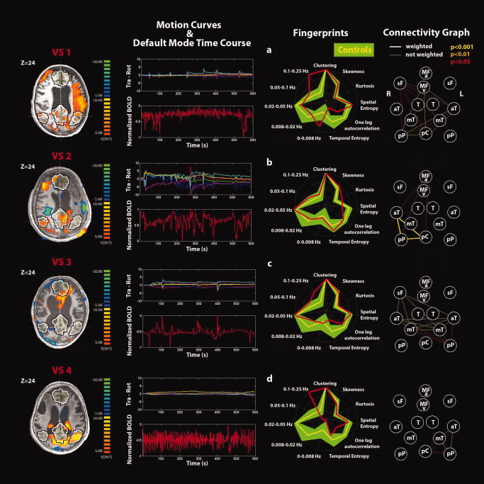
Single‐subject analyses identifying the default‐mode network (DMN) and connectivity graphs in (a–d) VS patients 1–4. See Figure 5 for explanatory legend. [Color figure can be viewed in the online issue, which is available at wileyonlinelibrary.com.]

Figure 7.

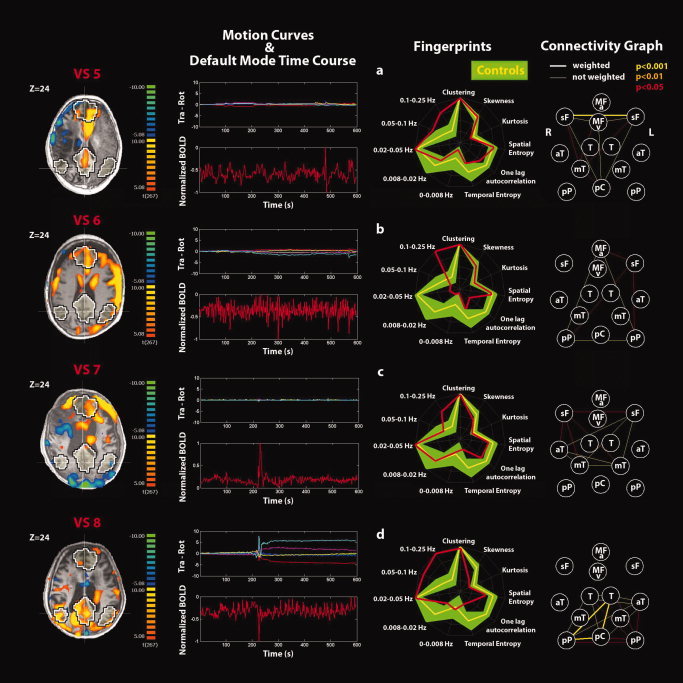
Single‐subject analyses identifying the default‐mode network (DMN) and connectivity graphs in (a–d) VS patients 5–8. See Figure 5 for explanatory legend. [Color figure can be viewed in the online issue, which is available at wileyonlinelibrary.com.]

A contrast T‐test map indicates the regions where the DMN time courses for controls and VS patients predicted in a significantly different way the BOLD signal with respect to the mean signal. The difference graph shows a connection between each pair of ROIs for which the sum of anticorrelation‐corrected beta values minus their difference is significantly different (permutation test) between controls and VS patients. The colors and thickness for the edges in the difference graph have the same meaning as in the mean graph.

RESULTS

Healthy Controls

In Group 2 of controls (see Table I in the Supporting Information), the three different connectivity ICA methods identified the same DMN at the single‐subject level. Cross validation with self‐organizing ICA showed concordance of the selected network in all healthy volunteers. In Group 3 of controls (see Table II in the Supporting Information), cross validation with self‐organizing ICA showed concordance of the selected network in six of eight healthy volunteers. The time course of the selected DMN showed a power spectrum peaking in the range of 0.02–0.05 Hz. At the group level (Fig. 4), the nodes showing the highest number of significant connections (edges surviving Bonferroni correction) were the ventral and anterior medial prefrontal cortices (number of edges = 7) followed by the precuneus/PCC (number of edges = 4), and left and right posterior parietal cortices (number of edges = 3). Healthy controls' mean spatial map identified the DMN pattern as shown in Figure 3. As confirmed by the connectivity graph, the regions that are the predominant representatives of the DMN are MFa and MFv, pC, L‐pP and R‐pP, and L‐sF and R‐sF.

Figure 4.

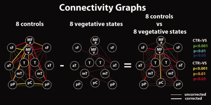
Connectivity graphs for the eight healthy controls and the eight VS patients' groups and between‐group differences. Red (blue), orange (cyan), and yellow (green) lines represent P = 0.05, P = 0.01, and P = 0.001, respectively, for positive and negative differences. Thicker lines are connections surviving correction for multiple comparisons. Nodes are defined as for Figure 1. [Color figure can be viewed in the online issue, which is available at wileyonlinelibrary.com.]

VS Patients' Group Data

VS patients' spatial map (Fig. 3) showed no significant pattern as also confirmed by the connectivity graph (time courses corresponding to the DMN selected by the second selection criterion have been used). The contrast control vs. VS patients' spatial map did not show any significant result when thresholded at false discovery rate corrected P < 0.05 within a DMN mask obtained from an independent dataset of healthy controls (Group 1). On the contrary, differences in connectivity graphs highlighted the connection between the MFv and the pC as well as between the MFv and the left and right lateral parietal, the L‐sF and R‐sF, the left anterior temporal gyrus, and the MFa. Compared with controls, VS patients' graphs showed a significantly lower total number of edges (numbers are approximated to integer, 41 ± 13, range 21–66 vs., respectively, for the three selection criteria: first: 17 ± 5, range 15–28, P < 0.001; second: 10 ± 4, range 6–15, P < 0.001; third: 14 ± 2, range 10–15, P < 0.001) as well as the anticorrelation index (0.72 ± 0.09, range 0.55–0.83 vs., respectively, for the three selection criteria: first: 0.57 ± 0.08, range 0.42–0.69, P = 0.004; second: 0.52 ± 0.10, range 0.41–0.65, P < 0.001; third: 0.56 ± 0.08, range 0.43–0.69, P = 0.003). Significant differences (which confirmed previous results) were observed in the total number of anticorrelation‐corrected edges (numbers are approximated to integer, 30 ± 12, range 14–53 vs., respectively, for the three selection criteria: first: 10 ± 2, range 8–12, P = 0.002; second: 3 ± 2, range 3–9, P < 0.001; third: 8 ± 2, range 4–10, P < 0.001) as well as total number of weighted edges (18 ± 10, range 4–29 vs., respectively, for the three selection criteria: first: 1 ± 2, range 0–6, P = 0.002; second: 1 ± 1, range 0–3, P = 0.002; third: 1 ± 2, range 0–6, P = 0.002). For the anticorrelation‐corrected scores, which summarized in a single number both spatial and temporal properties, compared with controls, VS patients showed a lower anticorrelation‐corrected score (numbers are approximated to integers, 21 ± 9, range 7–38 vs., respectively, for the three selection criteria: first: 2 ± 1, range 1–4, P < 0.001; second: 3 ± 1, range 1–5, P < 0.001; third: 3 ± 1, range 1–5, P < 0.001). The weight w _F, which is a measure of the nature of the IC selected [artifactual (low) vs. neuronal (high)], showed, compared with controls, lower values in VS patients (0.68 ± 0.14, range 0.47–0.84 vs., respectively, for the three selection criteria: first: 0.24 ± 0.07, range 0.16–0.36, P < 0.001; second: 0.48 ± 0.18, range 0.24–0.74, P = 0.03; third: 0.40 ± 0.19, range 0.16–0.70, P = 0.005). In Figure 3, the mean DMN fingerprint for controls (yellow line) showed the characteristic bird shape [De Martino et al., 2007] with a predominant frequency band of 0.02–0.05 Hz, high level of clustering, and one‐lag autocorrelation. The mean DMN fingerprint (DMN components were selected with the second selection criterion) for VS patients (cyan line) did not show a normal bird‐like shape but showed a predominant frequency of 0.1–0.25 Hz even if the contribution in the frequency band of 0.02–0.05 Hz was still important. Significant lower temporal entropy was also observed in VS patients with respect to healthy controls. Finally, VS patients moved in the scanner more than healthy volunteers showing compared with controls higher even if not significantly different “displacement” and “speed” (see Appendix for definition; displacement = 0.95 ± 0.67, range 0.2–2.2 vs. 2.3 ± 2.0, range 0.2–5.9, P = 0.11; speed = 0.07 ± 0.04, range 0.02–0.13 vs. 0.28 ± 0.30, range 0.08–0.96, P = 0.08).

Patients' Single‐Subject Analysis

Single‐subject analysis refers to the DMN selected using the second criterion. None of the VS patients showed a DMN with both the spatial and temporal patterns comparable with healthy controls see Fig. 5 for an example of healthy control and Figs. 6 and 7 for the VS patients. Rapid transient “clonic” movements were observed for all patients. Spatial maps showed periphery patterns characteristic of motion artifacts. Individual fingerprint analysis showed a shift toward the higher frequency bands (0.1–0.25 Hz) especially in VS patients 1, 4, 6, and 8. In patients 1 and 8, a contribution in the low frequency band (0.02–0.05 Hz) was also observed, whereas for patients 2, 3, 5, and 7, the component selected was dominated by a low frequency behavior (0.02–0.05 Hz). Graph analysis showed some residual connections (weighted edges) in patient 2 (between pC and right lateral parietal posterior and anterior temporal gyri), in patient 5 (between L‐sF and R‐sF), and in patient 8 (between pC and right lateral parietal posterior and L‐T). In patient 2, we also observed substantial movement throughout the recording with a highly correlated power spectrum of the BOLD time course and the motion parameter curves.

The two locked‐in patients (Fig. 5) showed near‐normal DMN connectivity spatial pattern despite substantial movement artifacts (the three selection criteria gave the same component). In the temporal domain, an increase in the high frequencies was observed for patient 1 even if the contribution in the frequency band (0.02–0.05 Hz) was preserved. For patient 2, a proper fingerprint was observed. The connectivity graphs were characterized, respectively, by 28 and 36 total number of edges and an anticorrelation index of 0.74 for both patients giving, respectively, 21 and 27 total number of anticorrelation‐corrected connections, which were not significantly different from healthy controls (P = 0.27) and counted 21 and 28 weighted edges (P = 0.25). The anticorrelation‐corrected scores were, respectively, 14.0 and 16.6 in line with healthy controls. The weight w _F with values 0.67 and 0.62 was also in the healthy volunteers' range. The MCS patient showed a proper DMN spatial pattern in the right hemisphere as also confirmed by the connectivity graph (Fig. 5). A proper time‐course behavior was also observed together with a proper fingerprint. The total number of edges was 10 (second and third selection criteria) with an anticorrelation index of 0.65 giving a number of anticorrelation‐corrected edges of 6.5, the weighted edges 6, and a score of 3.6 with the anticorrelation‐corrected edges and the anticorrelation‐corrected score consistent with VS patients, but with the weighted edges being lower of healthy controls and higher than VS patients. The weight w _F was consistent with healthy controls.

DISCUSSION

Here, we have assessed different methodologies aiming to identify the DMN based on spatial ICA in the challenging patient population of severe brain damage. Three different strategies were developed: (i) spatially pattern driven, (ii) based on an automatic masking driven by the fingerprint properties (time domain dominated), and (iii) based on a compromise between spatial and temporal properties. After testing that the three strategies selected the same DMN component on an independent group of 10 healthy controls, we confirmed the validity of the three strategies by comparing results with those obtained by running self‐organizing ICA as implemented in Brain Voyager (similar results were obtained by preprocessing data in SPM and running ICA in FSL and then comparing our selection criteria with the similarity or the goodness of fit tests with or without selecting components based on their power spectrum). We next applied our methodology to another independent group of 8 healthy controls, eight VS, two LIS, and one MCS patients. Each of the three connectivity spatial ICA strategies permitted to identify the DMN at the single‐subject level in a user‐independent manner. In the group of 8 healthy controls, the three methods identified the same component characterized by the typical spatial pattern of the DMN [Beckmann et al., 2005] accompanied by a corresponding time course with a power spectrum peaking in the range 0.02–0.05 Hz. Cross validation with self‐organizing ICA showed concordance of the selected network in six of eight healthy volunteers. In the two subjects where both methods disagreed, post hoc analysis showed that self‐organizing ICA identified a network with a spatial pattern resembling the DMN but with a time course peaking at higher frequency with respect to the time course of the network selected by our methodology, which was dominated by neuronal frequencies [e.g., 0.01–0.05 Hz, De Luca et al., 2006]. The DMN fingerprint confirmed the previously reported characteristic bird‐shaped pattern in all healthy controls with a predominant frequency band of 0.02–0.05 Hz, high level of clustering, and one‐lag autocorrelation [De Martino et al., 2007].

For VS patients, the three selection criteria did not agree on the selected component. To have an indication of which of the three criteria, which worked equally well in healthy subjects, could be the one with more selection power in highly pathological brains, we decided to test our three methods on a MCS patient. In this patient, the DMN was easily detectable by visual inspection of the spatial pattern together with the fingerprint. The presence of the DMN only in the right hemisphere was in accordance with cerebral metabolic PET data, suggesting a neuronal activity pattern consistent with healthy controls only in the right hemisphere. The finding that only the second and the third selection criteria were able to pick the right component as DMN in this patient may illustrate the advantage of these last two methods in highly pathological brains where spatial patterns may be partially destroyed. To detect residual patterns of neuronal activity, it is probably more important to give more or equal selecting power to time than to space. Given the obtained results, we decided to use the second selection criterion because its fingerprint‐based procedure guiding the automatic masking seemed promising to identify for the DMN a component with neuronal source. Using our second selection criterion, our method did not identify a single connection between DMN nodes, which reached statistical significance at the VS patient' group level and failed to show any significant voxel that showed a consistent pattern of DMN connectivity. The mean DMN fingerprint was not bird shape like (even if the second selection criterion gave the most similar fingerprint to healthy controls) but showed a predominant frequency of 0.1–0.25 Hz, which was significantly higher from that observed in healthy controls. It is important to stress that broadband ultra‐slow fluctuations (<0.1 Hz) in BOLD fMRI and in neuronal activity typically show a 1/f power profile [Nir et al., 2008] with no predominant frequency, whereas narrow‐band spontaneous fluctuations around 0.1 Hz (as observed in the VS group) have been shown to be implicated in non‐neuronal processes such as vasomotion [Mitra et al., 1997]. This shift toward higher frequencies in the DMN could be caused by pulse and respiration artifacts (and their aliasing) [De Luca et al., 2006]. With a TR of 2 s (corresponding to a sampling rate of 0.5 Hz and a Niquist frequency (N _f) of 0.25 Hz) aliasing may be an important source of artifact. For example, a respiratory rate of 12 breaths per minute (i.e., 0.2 Hz < N _f) will not be aliased, while its first harmonic of 0.4 Hz (i.e., >N _f) is aliased at |0.4–0.5 Hz| = 0.1 Hz. Similarly, a heart rate of (for example) 63 beats per minute (1.05 Hz) is aliased at |1.05–2*0.5 Hz| = 0.05 Hz appearing in the DMN characteristic frequency range. The frequency band that was lower in VS patients when compared with controls was 0.008–0.02 Hz possibly reflecting a decrease in DMN neuronal activity. The temporal entropy and one‐lag autocorrelation were also shown to be decreased in VS patients possibly explained by, respectively, movement artifacts and high‐frequency time‐course behavior caused by pulse and respiratory artifacts. The clustering, skewness, kurtosis, and spatial entropy were not different between VS patients and controls, presumably indicating that the spatial properties of neuronal DMN activity and artifacts (i.e., pulse, respiration, movement, and global effects) might be comparable. However, this does not imply that artifacts would show a similar spatial pattern as the DMN. When the DMN does not exist or some other component (e.g., motion, heart, or respiratory rate) gives a higher contribution to connectivity—even if a fingerprint‐driven selection criterion tends to suppress this scenario–then the artifactual IC provides an upper bound on the connectivity number of edges for the DMN (i.e., a component is de facto always selected).

The connectivity study showed no overlap between the number of “anticorrelation‐corrected connections” or edges in VS patients and in controls. Connectivity graph analysis identified anterior–posterior midline disconnections in VS, in line with previous studies emphasizing the critical role of the precuneus/PCC and mesiofrontal cortices in the emergence of conscious awareness [Boly et al., 2008; Vanhaudenhuyse & Noirhomme et al., 2010]. Indeed, these areas are among the most active brain regions in conscious waking [Gusnard et al., 2001] and are among the least metabolically active regions in VS [Laureys et al., 2004] and in other states of altered consciousness such as general anesthesia [Alkire and Miller, 2005], sleep [Maquet, 1997], hypnotic state [Rainville et al., 2002], or dementia [Minoshima et al., 1997]. It has been suggested that these richly connected multimodal medial associative areas are part of the neural network subserving consciousness [Baars et al., 2003] and self‐awareness [Hagmann et al., 2008; Laureys et al., 2007]. It is important to stress here that the difference in anticorrelation‐corrected connectivity measured between VS patients and healthy controls is a combined result of both the reduction in the positive correlation between the regions of the DMN and of the anticorrelation with the regions of the ECN. A reduction is in fact observed in both the number of edges and the anticorrelation index in VS patients with respect to healthy controls (see Table II in the Supporting Information).

At the single‐subject level, none of the VS patients showed a DMN with a spatial and temporal pattern that was comparable with that observed in healthy controls. It should be noted that only in patient VS2 as for the MCS patient the metabolic PET study reported a preserved neuronal activity only in the right hemisphere, which was the hemisphere showing a preserved DMN spatial pattern (as illustrated by the connectivity graph) and with a DMN time course consistent with neuronal activity. Individual fingerprint analysis showed a shift toward the higher frequency bands (0.1–0.25 Hz) in four of eight VS patients (VS cases 1, 4, 6, and 8; see Figs. 6a,d and 7b,d) possibly caused by pulse or respiration artifacts (or by their aliasing). Aliasing of pulse and respiration frequencies could also explain the increase in lower frequency bands observed in VS patients (VS 2, 3, 5, and 7) where normal DMN neural activity is known to peak (see Figs. 6b,c and 7a,c). However, in the absence of simultaneous recording of heart and respiratory rates during the fMRI acquisitions, this remains speculative and one cannot here formally exclude the presence of a neuronal contribution. Note that in addition to simultaneous recording of physiological parameters, future studies should use a shorter TR, which will strongly reduce the aliasing of high frequency (albeit covering a fewer number of slices). Graph analyses also showed some residual connections (corrected for global effects) in VS patient 2 (between pC and right lateral parietal posterior and right anterior temporal gyrus), in VS5 (between R‐sF and L‐sF), and VS8 (between pC and right lateral parietal posterior and L‐T). In our view, these results may not reflect residual DMN neuronal activity but can be explained by pulse, respiratory, and mainly movement artifacts. The particular case of VS2 deserves some more caution because of the consistency between the spatial pattern and the independent observed metabolic PET data (also clinically the patient was considered a borderline MCS case). Patient VS8 was the only VS patient that subsequently recovered minimal signs of consciousness.

Despite substantial movement artifacts, the two locked‐in patients showed in the spatial domain a near‐to‐normal DMN connectivity pattern. In the temporal domain, the movements caused for LIS1 an increase in the high frequency band without masking the neuronal contribution in the lower frequency bands. The graph analysis showed a connectivity pattern indistinguishable from that observed in healthy controls. The MCS patient showed a DMN pattern intermediate between healthy controls and VS patients, suggesting that the extracted variables used for individual graph analyses may offer a classification of the level of consciousness in these challenging patients—as has been shown at the group level [Vanhaudenhuyse & Noirhomme et al., 2010]. When dealing with DOC patients, major confounds in resting‐state fMRI acquisitions are movement, pulse, respiration (and their aliasing), and global‐effect artifacts [Soddu et al., 2011]. Future clinical studies should therefore perform simultaneous heart and respiratory rate recordings [Gray et al., 2009] and real movement monitoring.

Normalization procedures are also very important issues when dealing with severe brain injury and highly deformed or, especially for chronic cases, atrophied brains [Dai et al., 2008]. In this study, anatomical placements of all ROI positions were visually checked to make sure no artifactual signal from non‐neuronal ventricular or white matter structures was included. Finally, it is important to stress that our presented methodology cannot protect against the well‐known problem of oversplitting or undersplitting of brain networks, inherent to ICA. In the case of ICA decompositions, higher dimensionalities of the model have recently been advocated [Kiviniemi et al., 2009; Smith et al., 2009], although the robustness of a given level of decomposition relies on being supported by data quality. The highly pathological brains of DOC patients do not allow quite often having good‐quality BOLD data. Using a limited number of components for the ICA decomposition may then probably result in a better solution. For the above reasons, tackling DMN splitting issue remains a very methodological challenge.

CONCLUSION

Here, we proposed a user‐independent constrained connectivity ICA method with three different selection criteria based on spatial and temporal information permitting DMN component selection at the single‐subject level. When applied to healthy subjects, the three criteria (i.e., (i) spatially pattern driven, (ii) based on an automatic masking driven by the fingerprint properties (time domain dominated), and (iii) based on a compromise between spatial and temporal properties) selected the same component. When subsequently applied to a MCS patient with a “functional hemispherectomy,” two of three selection criteria were able to detect the proper component. This suggests that a method with an automatic masking (in which a growing number of nodes are repeatedly excluded from the network until the selected component satisfies the DMN BOLD fingerprint constraints) could be a successful approach to select components in highly pathological brains or in conditions where the network can possibly become highly disconnected such as in pharmacological coma [Boveroux et al., 2010]. Defining scores that summarize both spatial and temporal fingerprint properties offers a good compromise for DMN connectivity studies in clinical settings. When applied to a small cohort of VS patients, the presented methodology permitted to isolate the main sources of connectivity in the DMN regions and, in our view, ruled out convincing neuronal contributions. Future studies should validate these methodologies comparing their sensitivity on simulated data of pathological brains. The robustness of the methodology was illustrated here by the study of two LIS patients (showing important movement yet permitting extraction of near‐normal DMN connectivity) and of a MCS patient (showing a half‐functioning brain with similar results obtained by rsfMRI and metabolic PET studies). The proposed approach can also be extended to other networks with or without renouncing to the concept of anticorrelation‐corrected connectivity in the assessment of resting‐state fMRI in real‐life clinical settings.

Supporting information

Additional Supporting Information may be found in the online version of this article.

Supporting Information

Connectivity Graph and Anticorrelation‐Corrected Number of Edges

To study connectivity between each pair of target points, we implemented a new method, which is based on ICA followed by a GLM. After running ICA with 30 components, we used the corresponding time courses to regress in the BOLD signal in each of the 13 ROIs (average time course over the voxels belonging to the ROI). For each component, we obtained 13 parameter estimates (beta values) indicating the weight of each regressor and the corresponding T‐values:

where c is the contrast vector that isolates each IC, and X is the matrix with the predictors TC_IC. The anticorrelation‐corrected number of edges was obtained by multiplying the total number of edges of each graph by a weight “w,” which measures the anticorrelation of the DMN activity with the extrinsic system/ECN. The anticorrelation‐corrected number of edges E _AntiCC was then defined in terms of the number of edges E as:

where 〈T _extr〉 is the average of the five extrinsic ROIs T‐values, max(|T _extr|) is the maximum of the absolute value of the five extrinsic ROIs T‐values and ± signs hold, respectively, for the ICs 1–30 (minus sign) and for ICs 31–60 (plus sign). The anticorrelation index would be close to 0 if the activity in the extrinsic network highly correlates with the activity in the intrinsic network (〈T _extr〉/max(|T _extr|) subtracts to 1), e.g., a global signal, and close to 1 if the activity in the extrinsic network is anticorrelated with the activity in the DMN (〈T _extr〉/max(|T _extr|) sums up to 1), e.g., the DMN component.

Fingerprint and Anticorrelation‐Corrected Scores

A fingerprint (as in De Martino et al. [2007], the fingerprint reports normalized values, respectively, for: degree of clustering, skewness, kurtosis, spatial entropy as calculated from the distribution of the z values for the considered IC and one‐lag autocorrelation, temporal entropy, and the power of the five frequency bands [0–0.008, 0.008–0.02, 0.02–0.05, 0.05–0.1, and 0.1–0.25 Hz] as extracted from the time course of the considered IC) is calculated in Brain Voyager for each IC. As presented in the methods to drive the automatic masking or to build the anticorrelation‐corrected scores, a Euclidean distance in the fingerprint space is defined as:

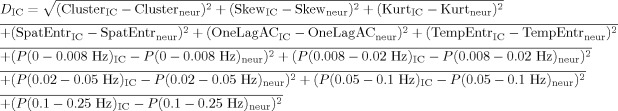using an average fingerprint with values “…_neur” built from the DMN components of the 11 healthy subjects (Group 1). The “anticorrelation‐corrected score” was built by multiplying the number of anticorrelation‐corrected edges by a new weight “w _F” defined by:

with w _F close to 0 for components that have a distance comparable with the max(D _IC) (“artifacts” components) and close to 1 for components with “neuronal” origin.

Motion Indices

Two motion indices were introduced describing the motion of patients compared with healthy controls. The first index Δ measures the mean over time of the displacement during the full acquisition (translation measured in millimeters and rotations measured in degrees). The second index Σ measures the mean over time of the displacement speed (variation over a repetition time) during the full acquisition:

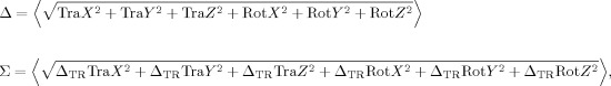where Δ_TR indicates the variation of a parameter over a TR.

REFERENCES

- Alkire MT, Miller J ( 2005): General anesthesia and the neural correlates of consciousness. Prog Brain Res 150: 229–244. [DOI] [PubMed] [Google Scholar]
- American Congress of Rehabilitation Medicine ( 1995): Recommendations for use of uniform nomenclature pertinent to patients with severe alterations in consciousness. Arch Phys Med Rehabil 76: 205–209. [DOI] [PubMed] [Google Scholar]
- Anand A, Li Y, Wang Y, Wu J, Gao S, Bukhari L, Mathews VP, Kalnin A, Lowe MJ ( 2005): Activity and connectivity of brain mood regulating circuit in depression: A functional magnetic resonance study. Biol Psychiatry 57: 1079–1088. [DOI] [PubMed] [Google Scholar]
- Baars BJ, Ramsoy TZ, Laureys S ( 2003): Brain, conscious experience and the observing self. Trends Neurosci 26: 671–675. [DOI] [PubMed] [Google Scholar]
- Beckmann CF, DeLuca M, Devlin JT, Smith SM ( 2005): Investigations into resting‐state connectivity using independent component analysis. Philos Trans R Soc Lond B Biol Sci 360: 1001–1013. [DOI] [PMC free article] [PubMed] [Google Scholar]
- Birn RM, Murphy K, Bandettini PA ( 2008): The effect of respiration variations on independent component analysis results of resting state functional connectivity. Hum Brain Mapp 29: 740–750. [DOI] [PMC free article] [PubMed] [Google Scholar]
- Biswal B, Yetkin FZ, Haughton VM, Hyde JS ( 1995): Functional connectivity in the motor cortex of resting human brain using echo‐planar MRI. Magn Reson Med 34: 537–541. [DOI] [PubMed] [Google Scholar]
- Boly M, Phillips C, Balteau E, Schnakers C, Degueldre C, Moonen G, Luxen A, Peigneux P, Faymonville ME, Maquet P, Laureys S ( 2008): Consciousness and cerebral baseline activity fluctuations. Hum Brain Mapp 29: 868–874. [DOI] [PMC free article] [PubMed] [Google Scholar]
- Boly M, Tshibanda L, Vanhaudenhuyse A, Noirhomme Q, Schnakers C, Ledoux D, Boveroux P, Garweg C, Lambermont B, Phillips C, Luxen A, Moonen G, Bassetti C, Maquet P, Laureys S ( 2009): Functional connectivity in the default network during resting state is preserved in a vegetative but not in a brain dead patient. Hum Brain Mapp 30: 2393–2400. [DOI] [PMC free article] [PubMed] [Google Scholar]
- Born JD, Albert A, Hans P, Bonnal J ( 1985): Relative prognostic value of best motor response and brain stem reflexes in patients with severe head injury. Neurosurgery 16: 595–601. [DOI] [PubMed] [Google Scholar]
- Boveroux P, Vanhaudenhuyse A, Bruno MA, Noirhomme Q, Lauwick S, Luxen A, Degueldre C, Plenevaux A, Schnakers C, Phillips C, Brichant JF, Bonhomme V, Maquet P, Greicius MD, Laureys S, Boly M ( 2010): Breakdown of within‐ and between‐network resting state functional magnetic resonance imaging connectivity during propofol‐induced loss of consciousness. Anesthesiology 113: 1038–1053. [DOI] [PubMed] [Google Scholar]
- Calhoun VD, Eichele T, Pearlson G ( 2009): Functional brain networks in schizophrenia: A review. Front Hum Neurosci 3: 17. [DOI] [PMC free article] [PubMed] [Google Scholar]
- Cole DM, Smith SM, Beckmann CF ( 2010): Advances and pitfalls in the analysis and interpretation of resting‐state FMRI data. Front Syst Neurosci 4: 8. [DOI] [PMC free article] [PubMed] [Google Scholar]
- Cordes D, Haughton VM, Arfanakis K, Wendt GJ, Turski PA, Moritz CH, et al. ( 2000): Mapping functionally related regions of brain with functional connectivity MR imaging. AJNR Am J Neuroradiol 21: 1636–1644. [PMC free article] [PubMed] [Google Scholar]
- Dai W, Carmichael OT, Lopez OL, Becker JT, Kuller LH, Gach HM ( 2008): Effects of image normalization on the statistical analysis of perfusion MRI in elderly brains. J Magn Reson Imaging 28: 1351–1360. [DOI] [PMC free article] [PubMed] [Google Scholar]
- Damoiseaux JS, Rombouts SA, Barkhof F, Scheltens P, Stam CJ, Smith SM, Beckmann CF ( 2006): Consistent resting‐state networks across healthy subjects. Proc Natl Acad Sci USA 103: 13848–13853. [DOI] [PMC free article] [PubMed] [Google Scholar]
- De Luca M, Beckmann CF, De Stefano N, Matthews PM, Smith SM ( 2006): fMRI resting state networks define distinct modes of long‐distance interactions in the human brain. Neuroimage 29: 1359–1367. [DOI] [PubMed] [Google Scholar]
- De Martino F, Gentile F, Esposito F, Balsi M, Di Salle F, Goebel R, Formisano E ( 2007): Classification of fMRI independent components using IC‐fingerprints and support vector machine classifiers. Neuroimage 34: 177–194. [DOI] [PubMed] [Google Scholar]
- Esposito F, Scarabino T, Hyvarinen A, Himberg J, Formisano E, Comani S, Tedeschi G, Goebel R, Seifritz E, Di Salle F ( 2005): Independent component analysis of fMRI group studies by self‐organizing clustering. Neuroimage 25: 193–205. [DOI] [PubMed] [Google Scholar]
- Esposito F, Aragri A, Pesaresi I, Cirillo S, Tedeschi G, Marciano E, Goebel R, Di Salle F ( 2008): Independent component model of the default‐mode brain function: Combining individual‐level and population‐level analyses in resting‐state fMRI. Magn Reson Imaging 26: 905–913. [DOI] [PubMed] [Google Scholar]
- Fair DA, Cohen AL, Dosenbach NU, Church JA, Miezin FM, Barch DM, Raichle ME, Petersen SE, Schlaggar BL ( 2008): The maturing architecture of the brain's default network. Proc Natl Acad Sci USA 105: 4028–4032. [DOI] [PMC free article] [PubMed] [Google Scholar]
- Formisano E, Esposito F, Di Salle F, Goebel R ( 2004): Cortex‐based independent component analysis of fMRI time series. Magn Reson Imaging 22: 1493–1504. [DOI] [PubMed] [Google Scholar]
- Fox MD, Raichle ME ( 2007): Spontaneous fluctuations in brain activity observed with functional magnetic resonance imaging. Nat Rev Neurosci 8: 700–711. [DOI] [PubMed] [Google Scholar]
- Fox MD, Snyder AZ, Vincent JL, Corbetta M, Van Essen DC, Raichle ME ( 2005): The human brain is intrinsically organized into dynamic, anticorrelated functional networks. Proc Natl Acad Sci USA 102: 9673–9678. [DOI] [PMC free article] [PubMed] [Google Scholar]
- Fox MD, Zhang D, Snyder AZ, Raichle ME ( 2009): The global signal and observed anticorrelated resting state brain networks. J Neurophysiol 101: 3270–3283. [DOI] [PMC free article] [PubMed] [Google Scholar]
- Giacino JT, Kalmar K, Whyte J ( 2004): The JFK Coma Recovery Scale‐Revised: Measurement characteristics and diagnostic utility. Arch Phys Med Rehabil 85: 2020–2029. [DOI] [PubMed] [Google Scholar]
- Golland Y, Bentin S, Gelbard H, Benjamini Y, Heller R, Nir Y, Hasson U, Malach R ( 2007): Extrinsic and intrinsic systems in the posterior cortex of the human brain revealed during natural sensory stimulation. Cereb Cortex 17: 766–777. [DOI] [PubMed] [Google Scholar]
- Golland Y, Golland P, Bentin S, Malach R ( 2008): Data‐driven clustering reveals a fundamental subdivision of the human cortex into two global systems. Neuropsychologia 46: 540–553. [DOI] [PMC free article] [PubMed] [Google Scholar]
- Gray MA, Minati L, Harrison NA, Gianaros PJ, Napadow V, Critchley HD ( 2009): Physiological recordings: Basic concepts and implementation during functional magnetic resonance imaging. Neuroimage 47: 1105–1115. [DOI] [PMC free article] [PubMed] [Google Scholar]
- Greicius MD, Menon V ( 2004): Default‐mode activity during a passive sensory task: Uncoupled from deactivation but impacting activation. J Cogn Neurosci 16: 1484–1492. [DOI] [PubMed] [Google Scholar]
- Greicius MD, Krasnow B, Reiss AL, Menon V ( 2003): Functional connectivity in the resting brain: A network analysis of the default mode hypothesis. Proc Natl Acad Sci USA 100: 253–258. [DOI] [PMC free article] [PubMed] [Google Scholar]
- Greicius MD, Srivastava G, Reiss AL, Menon V ( 2004): Default‐mode network activity distinguishes Alzheimer's disease from healthy aging: Evidence from functional MRI. Proc Natl Acad Sci USA 101: 4637–4642. [DOI] [PMC free article] [PubMed] [Google Scholar]
- Gusnard DA, Akbudak E, Shulman GL, Raichle ME ( 2001): Medial prefrontal cortex and self‐referential mental activity: Relation to a default mode of brain function. Proc Natl Acad Sci USA 98: 4259–4264. [DOI] [PMC free article] [PubMed] [Google Scholar]
- Hagmann P, Cammoun L, Gigandet X, Gerhard S, Ellen Grant P, Wedeen V, Meuli R, Thiran JP, Honey CJ, Sporns O ( 2008): Mapping the structural core of human cerebral cortex. PLoS Biol 6: e159. [DOI] [PMC free article] [PubMed] [Google Scholar]
- Hyvarinen A, Karhunen J, Oja E ( 2001): Independent Component Analysis. John Wiley & Sons. [Google Scholar]
- Jafri MJ, Pearlson GD, Stevens M, Calhoun VD ( 2008): A method for functional network connectivity among spatially independent resting‐state components in schizophrenia. Neuroimage 39: 1666–1681. [DOI] [PMC free article] [PubMed] [Google Scholar]
- Kennedy DP, Redcay E, Courchesne E ( 2006): Failing to deactivate: Resting functional abnormalities in autism. Proc Natl Acad Sci USA 103: 8275–8280. [DOI] [PMC free article] [PubMed] [Google Scholar]
- Kiviniemi V, Kantola JH, Jauhiainen J, Hyvärinen A, Tervonen O ( 2003): Independent component analysis of nondeterministic fMRI signal sources. Neuroimage 19: 253–260. [DOI] [PubMed] [Google Scholar]
- Kiviniemi V, Starck T, Remes J, Long X, Nikkinen J, Haapea M, Veijola J, Moilanen I, Isohanni M, Zang YF, Tervonen O ( 2009): Functional segmentation of the brain cortex using high model order group PICA. Hum Brain Mapp 30: 3865–3886. [DOI] [PMC free article] [PubMed] [Google Scholar]
- Koch W, Teipel S, Mueller S, Buerger K, Bokde ALW, Hampel H, Coates U, Reiser M ( 2010): Effects of aging on default mode network activity in resting state fMRI: Does the method of analysis matter? Neuroimage 15: 280–287. [DOI] [PubMed] [Google Scholar]
- Laureys S, Owen AM, Schiff ND ( 2004): Brain function in coma, vegetative state, and related disorders. Lancet Neurol 3: 537–546. [DOI] [PubMed] [Google Scholar]
- Laureys S, Perrin F, Bredart S ( 2007): Self‐consciousness in non‐communicative patients. Conscious Cogn 16: 722–741; discussion 742–725. [DOI] [PubMed] [Google Scholar]
- Lowe MJ, Mock BJ, Sorenson JA ( 1998): Functional connectivity in single and multislice echoplanar imaging using resting‐state fluctuations. Neuroimage 7: 119–132. [DOI] [PubMed] [Google Scholar]
- Lowe MJ, Phillips MD, Lurito JT, Mattson D, Dzemidzic M, Mathews VP ( 2002): Multiple sclerosis: Low‐frequency temporal blood oxygen level‐dependent fluctuations indicate reduced functional connectivity initial results. Radiology 224: 184–192. [DOI] [PubMed] [Google Scholar]
- Maquet P ( 1997): Positron emission tomography studies of sleep and sleep disorders. J Neurol 244: S23–S28. [DOI] [PubMed] [Google Scholar]
- McKeown MJ, Makeig S, Brown GG, Jung TP, Kindermann SS, Bell AJ, Sejnowski T ( 1998): Analysis of fMRI data by blind separation into independent spatial components. Hum Brain Mapp 6: 160–188. [DOI] [PMC free article] [PubMed] [Google Scholar]
- Meindl T, Teipel S, Elmouden R, Mueller S, Koch W, Dietrich O, Coates U, Reiser M, Glaser C ( 2010): Test‐retest reproducibility of the default‐mode network in healthy individuals. Hum Brain Mapp 31: 237–246. [DOI] [PMC free article] [PubMed] [Google Scholar]
- Minoshima S, Giordani B, Berent S, Frey KA, Foster NL, Kuhl DE ( 1997): Metabolic reduction in the posterior cingulate cortex in very early Alzheimer's disease. Ann Neurol 42: 85–94. [DOI] [PubMed] [Google Scholar]
- Mitra PP, Ogawa S, Hu X, Ugurbil K ( 1997): The nature of spatiotemporal changes in cerebral hemodynamics as manifested in functional magnetic resonance imaging. Magn Reson Med 37: 511–518. [DOI] [PubMed] [Google Scholar]
- Murphy K, Birn RM, Handwerker DA, Jones TB, Bandettini PA ( 2009): The impact of global signal regression on resting state correlations: Are anti‐correlated networks introduced? Neuroimage 44: 893–905. [DOI] [PMC free article] [PubMed] [Google Scholar]
- Nir Y, Hasson U, Levy I, Yeshurun Y, Malach R ( 2006): Widespread functional connectivity and fMRI fluctuations in human visual cortex in the absence of visual stimulation. Neuroimage 30: 1313–1324. [DOI] [PubMed] [Google Scholar]
- Nir Y, Mukamel R, Dinstein I, Privman E, Harel M, Fisch L, Gelbard‐Sagiv H, Kipervasser S, Andelman F, Neufeld MY, Kramer U, Arieli A, Fried I, Malach R ( 2008): Interhemispheric correlations of slow spontaneous neuronal fluctuations revealed in human sensory cortex. Nat Neurosci 11: 1100–1108. [DOI] [PMC free article] [PubMed] [Google Scholar]
- Perlbarg V, Marrelec G ( 2008): Contribution of exploratory methods to the investigation of extended large‐scale brain networks in functional MRI: Methodologies, results, and challenges. Int J Biomed Imaging 2008: 218519. [DOI] [PMC free article] [PubMed] [Google Scholar]
- Perlbarg V, Bellec P, Anton JL, Pelegrini‐Issac M, Doyon J, Benali H ( 2007): CORSICA: Correction of structured noise in fMRI by automatic identification of ICA components. Magn Reson Imaging 25: 35–46. [DOI] [PubMed] [Google Scholar]
- Rainville P, Hofbauer RK, Bushnell MC, Duncan GH, Price DD ( 2002): Hypnosis modulates activity in brain structures involved in the regulation of consciousness. J Cogn Neurosci 14: 887–901. [DOI] [PubMed] [Google Scholar]
- Rombouts SA, Damoiseaux JS, Goekoop R, Barkhof F, Scheltens P, Smith SM, Beckmann CF ( 2009): Model‐free group analysis shows altered BOLD FMRI networks in dementia. Hum Brain Mapp 30: 256–266. [DOI] [PMC free article] [PubMed] [Google Scholar]
- Schilbach L, Eickhoff SB, Rotarska‐Jagiela A, Fink GR, Vogeley K ( 2008): Minds at rest? Social cognition as the default mode of cognizing and its putative relationship to the “default system” of the brain. Conscious Cogn 17: 457–467. [DOI] [PubMed] [Google Scholar]
- Smith SM, Fox PT, Miller KL, Glahn DC, Fox PM, Mackay CE, Filippini N, Watkins KE, Toro R, Laird AR, Beckmann CF ( 2009): Correspondence of the brain's functional architecture during activation and rest. Proc Natl Acad Sci USA 106: 13040–13045. [DOI] [PMC free article] [PubMed] [Google Scholar]
- Soddu A, Vanhaudenhuyse A, Demertzi A, Bruno MA, Tshibanda L, Di H, Boly M, Papa M, Laureys S, Noirhomme Q: Resting state activity in patients with disorders of consciousness. Funct Neurol 2011. (in press). [PMC free article] [PubMed] [Google Scholar]
- The Multi‐Society Task Force on PVS ( 1994): Medical aspects of the persistent vegetative state (1). N Engl J Med 330: 1499–1508. [DOI] [PubMed] [Google Scholar]
- Vanhaudenhuyse A, Noirhomme Q, Tshibanda LJ, Bruno MA, Boveroux P, Schnakers C, Soddu A, Perlbarg V, Ledoux D, Brichant JF, Moonen G, Maquet P, Greicius MD, Laureys S, Boly M ( 2010): Default network connectivity reflects the level of consciousness in non‐communicative brain‐damaged patients. Brain 133: 161–171. [DOI] [PMC free article] [PubMed] [Google Scholar]
- Vanhaudenhuyse A, Demertzi A, Schabus M, Noirhomme Q, Bredart S, Boly M, Phillips C, Soddu A, Luxen A, Moonen G, Laureys S ( 2011): Two distinct neuronal networks mediate the awareness of environment and of self. J Cogn Neurosci 23(3):570–578. [DOI] [PubMed] [Google Scholar]
- Vincent JL, Patel GH, Fox MD, Snyder AZ, Baker JT, Van Essen DC, Zempel JM, Snyder LH, Corbetta M, Raichle ME ( 2007): Intrinsic functional architecture in the anaesthetized monkey brain. Nature 447: 83–86. [DOI] [PubMed] [Google Scholar]
- Weissman‐Fogel I, Moayedi M, Taylor KS, Pope G, Davis KD ( 2010): Cognitive and default‐mode resting state networks: Do male and female brains “rest” differently? Hum Brain Mapp 31: 1713–1726. [DOI] [PMC free article] [PubMed] [Google Scholar]
- Xiong J, Parsons LM, Gao JH, Fox PT ( 1999): Interregional connectivity to primary motor cortex revealed using MRI resting state images. Hum Brain Mapp 8: 151–156. [DOI] [PMC free article] [PubMed] [Google Scholar]
- Yang H, Long XY, Yang Y, Yan H, Zhu CZ, Zhou XP, Zang YF, Gong QY ( 2007): Amplitude of low frequency fluctuation within visual areas revealed by resting‐state functional MRI. Neuroimage 36: 144–152. [DOI] [PubMed] [Google Scholar]
- Ylipaavalniemi J, Vigario R ( 2008): Analyzing consistency of independent components: An fMRI illustration. Neuroimage 39: 169–180. [DOI] [PubMed] [Google Scholar]
Associated Data
This section collects any data citations, data availability statements, or supplementary materials included in this article.
Supplementary Materials