

Abstract
Previously, we introduced the use of individual cortical location and orientation constraints in the spatiotemporal Bayesian dipole analysis setting proposed by Jun et al. ([2005]; Neuroimage 28:84–98). However, the model's performance was limited by slow convergence and multimodality of the numerically estimated posterior distribution. In this paper, we present an intuitive way to exploit functional magnetic resonance imaging (fMRI) data in the Markov chain Monte Carlo sampling ‐based inverse estimation of magnetoencephalographic (MEG) data. We used simulated MEG and fMRI data to show that the convergence and localization accuracy of the method is significantly improved with the help of fMRI‐guided proposal distributions. We further demonstrate, using an identical visual stimulation paradigm in both fMRI and MEG, the usefulness of this type of automated approach when investigating activation patterns with several spatially close and temporally overlapping sources. Theoretically, the MEG inverse estimates are not biased and should yield the same results even without fMRI information, however, in practice the multimodality of the posterior distribution causes problems due to the limited mixing properties of the sampler. On this account, the algorithm acts perhaps more as a stochastic optimizer than enables a full Bayesian posterior analysis. Hum Brain Mapp 2009. © 2008 Wiley‐Liss, Inc.
INTRODUCTION
Since the development of functional magnetic resonance imaging (fMRI) the noninvasive study of human visual processing hierarchy has been of specific interest to researchers. The experiments range from first seminal studies demonstrating the feasibility of acquiring magnetic resonance signals related to increased blood flow and/or blood oxygenation level dependent (BOLD) contrast [Belliveau et al.,1991; Kwong et al.,1992; Ogawa et al.,1992] to more complex mappings of representations of the visual fields in human cerebral cortex [DeYoe et al.,1996], and to accurate mappings of borders and sizes of human retinotopic visual areas—V1, V2, VP, V3, and V4 [ Dougherty et al.,2003; Sereno et al.,1995]. Functional imaging has also been used to study areas with operational specialization, such as V5 which is sensitive to visual motion [Watson et al.,1993]. It is also known that V1 of humans responds well to patterned flickering stimuli [Engel et al.,1997] and hence checkerboard stimuli have traditionally been used to map the borders of the visual areas. In phase‐encoded mapping, slowly changing position of flickering checkerboard stimuli determines the polar angle of activation on the cortex, whereas a flickering and moving ring reveals the retinotopic organization with respect to eccentricity [Engel et al.,1997; Dougherty et al.,2003]. Recently, Vanni et al. [2005] developed a multifocal mapping method for fMRI that enables rapid and direct spatial exploration of multiple local visual field representations and gives complementary information to phase‐encoded mappings of retinotopic areas.
There is accumulating evidence that the human visual system is anatomically and functionally organized not only for bottom‐up hierarchical processing but also for top‐down modulation of activity with higher cognitive tasks [Courtney and Ungerleider,1997]. Thus, it is crucial that the analysis methods evolve to the direction of providing more accurate information of this visual processing network, both in the spatial and temporal domain, the latter benefiting from data provided by electroencephalography (EEG) and/or magnetoencephalography (MEG) [see, e.g., Hämäläinen et al.,1993; Nunez,1981, for a review on EEG and MEG]. Since the MEG/EEG inverse problem is ill‐posed [Sarvas,1987], spatial fMRI information is potentially useful in resolving the ambiguity. Often, because of difficulties in the true multimodal integration of MEG/EEG and fMRI, the suggested solutions have been for instance direct comparison of the separate results [e.g., Ahlfors et al.,1999], using fMRI data as a basis to adjust the source variance parameters [Dale et al.,2000; Liu et al.,1998], utilization of the functional results for constraining the possible source positions [e.g., Korvenoja et al.,1999], or by directly seeding the fMRI locations and cortical orientations to be optimized with a suitable EEG source dipole model [Vanni et al.,2004a,b]. Lately, there has been great interest in Bayesian methods utilizing fMRI prior information, for instance, with distributed linear solutions of the MEG/EEG inverse problem [e.g., Dale et al.,2000; Phillips et al.,2005] and also on determining the relevance of the fMRI prior information included in the inverse solution [Daunizeau et al.,2005].
The usefulness of Bayesian inference [Bernardo and Smith,1994; Gelman et al.,2003] has recently been demonstrated in localizing electromagnetic brain activity [e.g., Baillet and Garnero,1997; Friston et al.,2002a,b; Phillips et al.,1997; Schmidt et al.,2000]. A Bayesian solution to the inverse problem is formally expressed in the form of posterior probability distribution for the parameters of interest, such as dipole location and amplitude. Particularly, with electromagnetic inverse estimation problems, the posterior distribution cannot be often obtained in closed form and one of the many Markov chain Monte Carlo (MCMC) sampling schemes available [e.g., Gilks et al.,1996] is employed to numerically perform the high dimensional integrations involved in the posterior analysis [Auranen et al.,2005; Bertrand et al.,2001; Jun et al.,2005; Kincses et al.,2003; Schmidt et al., 1999,2000].
The efficiency of this so‐called MCMC sampling can be evaluated not only by the physiological meaningfulness of the localization results, but also by the convergence of the sampling algorithm, which is characterized, for instance, by the number of iterations required before the drawn samples are representatives of the true posterior distribution. Also, the sampling method might not be optimal for switching between different solutions modes of a Markov chain when the posterior distribution is multimodal. If the sampler does not switch well between modes, it is very difficult to validly compare the probability mass of the different solution modes (i.e., inverse estimates) as samples from the different chains are not typically directly comparable. Previously, we implemented cortical orientation and location constraints to a Bayesian dipole analysis model introduced by Jun et al. [2005] and showed that it provides reasonable inverse estimates with little manual intervention [Auranen et al.,2007]. However, the convergence of the Markov chain was rather slow and the sampler did not switch optimally between different modes, thus hampering full Bayesian posterior analysis.
In this article, we incorporate fMRI data to our cortically constrained MEG inverse dipole sampling method [Auranen et al.,2007], not by directly seeding the model or by using strict priors, but by introducing fMRI‐based proposal distributions that are used to suggest MCMC jumps to more likely activated cortical locations. This yields an fMRI‐guided MEG inverse model, which we first verify by simulations designed to test the ability of our fMRI‐guided dipole sampling to produce improved localization results and faster convergence than the model without fMRI‐guidance. With an empirical MEG/fMRI dataset, we start by marking the position of the individual retinotopic areas of the subjects with fMRI multifocal stimulation and then use the fMRI data gathered during the presentation of a drifting grating visual stimulus to test our fMRI‐guided MCMC sampling procedure for MEG inverse modeling. With the visual areas revealed by fMRI multifocal mapping, we are able to make a qualitative assessment of the drifting grating MEG inverse dipole locations.
As our previous model [Auranen et al.,2007] produces reasonable estimates with sources far apart from each other, we wanted to test the model in a particularly difficult situation, namely to scan the locations of human visual system, in which the sources are known to be adjacent [Vanni et al.,2004b] making the inverse estimation challenging. We specifically hypothesize that with simulated data, the convergence of the sampling procedure is faster and the results are both qualitatively and quantitatively improved with the fMRI‐guided MEG inverse dipole modeling. With the empirical visual motion data, the number of iterations required for convergence is slightly smaller although both methods produce qualitatively similar results.
MATERIALS AND METHODS
The Experiments
Three male subjects (ages: 33, 27, 29) with normal or corrected‐to‐normal vision participated in both the multifocal fMRI experiment and in the drifting grating experiment, that was performed in both fMRI and MEG. The multifocal experiment was conducted for localizing the approximate borders of retinotopic areas for the qualitative evaluation of the fMRI‐guided MEG source localization results on individual level. The drifting grating experiment was designed to produce simple, well‐localized hierarchical activity patterns in the low‐ and middle‐tier (V5/MT) visual areas of the right hemisphere. In all the experiments, the subjects were instructed to passively fixate on the fixation mark at the center of the screen. High‐resolution T 1‐weighted 3D anatomical MR images were obtained using 3 T scanner (General Electric Signa, Milwaukee, WI; located at Helsinki University of Technology, Finland) and 1.5 T scanners (Siemens Sonata and Vision, Erlangen, Germany; located at Massachusetts General Hospital, USA and Helsinki University Central Hospital, Finland, respectively). The anatomical images were used for visualization and for the source space and boundary‐element model (BEM) surface reconstructions. All functional MRI stacks were acquired with the GE 3 T scanner.
Multifocal fMRI
The multifocal stimuli (see Fig. 1) consisted of eight regions of flickering checkerboard stimuli on the horizontal and vertical meridian with 11 combinations, so that the stimulus sequences of all regions are orthogonal in the design matrix of the general linear model [for details of the multifocal mapping scheme, see, Vanni et al.,2005]. During two separate runs, 244 functional T 2*‐weighted volumes depicting BOLD contrast were acquired with 24 slices, slice thickness and in‐slice resolution of 2.5 mm, aligned perpendicular to the parieto‐occipital sulcus in the sagittal image giving a good sampling over the whole occipital lobe (EPI sequence, TR 1819 ms, TE 30 ms, flip angle 60, FOV 16, matrix size 64 × 64).
Figure 1.

Left: Three examples of the fMRI multifocal stimuli. Right: A snapshot of the drifting grating stimulus (fMRI). The subjects were fixating on the center of the screen.
Drifting Grating fMRI
Although a patterned flickering stimuli might provide the best responses in V1, we utilized drifting grating stimulus that might also produce detectable activation higher in the hierarchy of visual system extending to V5. The drifting grating covered a 60° polar sector in the middle of the lower left quadrant of the visual field with 2°–7° eccentricity (see Fig. 1). The spatial frequency at 4.5° eccentricity (i.e., the mean spatial frequency of the grating) was 1.3 cycles/degree. Drifting speed was 7.4° per second, but only one cycle was presented with stimulus duration of 107 ms. The experiment was a passive block design with alternating 50 s rest and stimulation periods. The 107 ms stimulus (4 images in a row, each 27 ms) was presented with varying ISI of 0.8–1.2 s. During three separate runs, 308 functional volumes were acquired with 27 slices, slice thickness and in‐slice resolution of 3.0 mm, aligned perpendicular to the parieto‐occipital sulcus to cover all of the visual areas (EPI sequence, TR 2,000 ms, TE 30 ms, flip angle 60, FOV 19, matrix size 64 × 64).
The multifocal fMRI was designed for good resolution mapping of the retinotopic visual areas, which are localized in the occipital lobes. In the drifting grating experiment, we wanted to detect activation everywhere in the visually responsive areas covering not only occipital lobe, but also parietal lobe, and parts of the temporal and frontal lobes. For this, we were obliged to sample a larger space, affecting the selected parameters (number of slices, slice thickness, in‐slice resolution, FOV, and TR) in comparison to the multifocal fMRI experiment.
Drifting Grating MEG
The MEG data were gathered in a magnetically shielded room with a Vectorview MEG system (Elekta‐Neuromag Oy, Helsinki, Finland) located at Helsinki University of Technology, Finland. Exactly the same design was used in fMRI and MEG acquisition resulting in over 800 (electro‐oculogram) artefact‐free trials for each subject. The data were collected with 600 Hz sampling frequency and downsampled to 300 Hz, notch filtered for 50‐Hz noise, and high‐pass (Butterworth) filtered with corner frequency of 0.2 Hz prior to averaging and further analyses. The averaged MEG evoked fields for the drifting grating experiment are shown in Figure 2. Since the high‐pass filter ensured the chopping of slow drifting effects in the data, baseline correction was not necessary, and if used, the correction itself might cause unexpected effects upon the model. With baseline correction, the relative amplitudes of the channels at the beginning of a time window would be pitched to a specific level, which would be inconsistent with the full spatiotemporal noise structure of the measurements. During MEG measurements the stimulus had the same size, position, spatial frequency, luminance, and contrast as the stimulus in the magnet. Because of different refresh rates with the data projectors, in MEG the stimulus duration was 134 ms (4 images, each 34 ms) with drifting speed of 5.9° per second. However, we consider this difference to be insignificant for this stimulus type.
Figure 2.
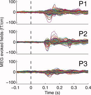
The averaged MEG evoked fields for all the subjects. Number of artefact‐free trials per subject was over 800. One line in each of the graphs represents one channel in the MEG sensor array. Notably, subject P3 had the worst signal to noise ratio. [Color figure can be viewed in the online issue, which is available at www.interscience.wiley.com.]
Initial Processing of fMRI, MRI, and MEG Data
The fMRI analysis in both experiments was carried out using FEAT version 5.63 of the FSL software tools [Smith et al.,2004]. The following prestatistic processing was used: slice time correction, high‐pass temporal filtering, MCFLIRT [Jenkinson et al.,2002] was applied for motion correction, and FLIRT [Jenkinson and Smith,2001; Jenkinson et al.,2002] for aligning the functional stacks with high resolution anatomical images (along with manual adjustments). Neither intensity normalization nor spatial smoothing was used in order to maximize the resolution of the data projection on the cortical surface reconstructions. On each individual, the first level time‐series statistical analysis was carried out using FILM with local autocorrelation correction [Woolrich et al.,2001] and the Z statistic images were thresholded by Z > 5 and a clusterwise significance of P = 0.05 [Worsley et al.,1992]. To combine different scanning sessions, higher‐level fixed effects analysis was performed by forcing the random effects variance to zero in FLAME [Beckmann et al.,2003; Woolrich et al.,2004].
For MEG forward and inverse modeling, the anatomical MRI data sets were processed with the Freesurfer software [Dale et al.,1999; Fischl et al.,1999]. The geometry of the white‐gray matter surface was derived with an automatic segmentation algorithm to yield a triangulated model with approximate 340,000 vertices [Dale et al.,1999; Fischl et al., 1999,2001]. This dense triangulation was decimated to a grid size of about 35,000 points. Using the MNE software (http://www.nmr.mgh.harvard.edu/martinos/userInfo/data/sofMNE.php), we calculated the magnetic field produced by current dipoles oriented normal to the cortical mantle at the decimated white‐gray matter surface vertex locations. In the forward calculations, we employed a single‐compartment BEM [e.g., Mosher et al.,1999]. All MEG data preprocessing and processing were conducted in MATLAB (The MathWorks, Natick, MA).
Simulated Data
For simulations, we utilized three source locations on the right occipital areas of subject P1 (Fig. 3A). The simulated dipolar sources had a 20‐nAm strength and different time courses with realistic measurement noise added based on empirical data [see, Auranen et al.,2007]. By slightly varying the location of two sources (2–3 mm along the cortex) the orientation changed significantly enough to make some of the sources barely visible in MEG sensors due to their almost radial orientation (S1r and S2r). This resulted in four different dipole configurations (I–IV) of the three sources S1, S2, and S3, so that in the first case (I) the sources were all well visible on the sensors, in the second case (II) one of the sources, S2r, was in practice covered by measurement noise and source S1, in the third case (III) source S1r was only somewhat visible due to orientation whereas the last case (IV) had the two previous cases combined. In the fourth case, practically only source S3 expressed clearly onto the sensor data producing visible fields (Fig. 3C).
Figure 3.

(A) Simulated source locations and timecourses. The orientations of the sources simulated using the real 3D white‐gray matter surface are visualized on the inflated cortical surface to reveal the clear difference in orientation between S1/S2 with S1r/S2r, respectively. (B) Simulated fMRI data used to generate different proposal distributions for the fMRI‐guided sampler. (C) The MEG fields produced by four different simulated dipole configurations. The sensor array consists of two planar gradiometers measuring the magnetic field gradient in two orthogonal directions on 102 locations around the head. There are clear differences in the expression of the sources to the sensors because of slight orientation differences. [Color figure can be viewed in the online issue, which is available at www.interscience.wiley.com.]
Simulated fMRI data used to construct the proposal distributions for the MCMC sampling scheme were produced by simple extended Gaussian kernels enveloping the actual dipole locations on the source space surface (Fig. 3B). We assessed the model with the four abovementioned simulated dipole configurations using five different proposal distributions: no guidance, correct fMRI‐guidance, an extra kernel, one of the locations missing, and one of the locations falsely localized, in order to reveal the differences with or without the guided sampling procedure and with small discrepancies in the proposal distribution.
Model Overview
To avoid shifting the focus from the novel idea of utilizing fMRI data for guiding the MCMC‐based algorithm, and to keep the manuscript straightforward, we do not duplicate the model formulation from [Auranen et al.,2007]. Here, the simulated and empirical data were analyzed with this previously described model with modifications so that the fMRI‐guidance in the form of proposal distributions in the reversible jump Markov chain Monte Carlo and Metropolis‐Hastings parts of the sampling procedure could be used [see, next section and Auranen et al.,2007, for details].
In this article, we employed both our singular value decomposition (SVD) ‐based strategy and the speed‐up strategy proposed by Jun et al. [2005], which uses a low‐rank approximation of the temporal current correlation obtained by eliminating negligible eigenvalues. The SVD speed‐up and regularization reduces the effective number of MEG measurements by using only the most important linearly independent channel combinations based on signal‐to‐noise ratio (SNR). These two actions help to accelerate the sampling procedure considerably without significantly biasing the results. This is crucial as we are analyzing relatively long segments of empirical data (500 ms) with a downsampled sampling rate of 300 Hz resulting to about 150 timepoints.
As minor computational upgrades to our previous model, we adaptively store to memory some of the intermediate computations that need to be calculated several times during sampling. The actual parametrization of the dipole location parameters using spherical angles is also modified in order to enable the use of the discrete fMRI proposal distributions.
The utilized source space consists of white‐gray matter boundary with sources oriented normal to the surface. This corresponds to the direction of the net current in the gray matter. The source space was discretized with ∼8,000 points for all the subjects in the inverse estimation.
fMRI‐Based Proposal Distribution
The fMRI‐guidance is implemented by creating proposal distributions of probable source locations from the empirical fMRI data by utilizing the Freesurfer software. In this, the functional volumes or more exactly, the statistical parametric maps are aligned with the anatomical stacks and the activations are projected and rendered to the source space of cortical white‐gray matter surface. As a result, we arrive with a vector of values (i.e., the proposal distribution), each element depicting the Z‐score in one vertex point of the source space. The active surface locations of the propoal distribution were directly assigned the corresponding Z‐score value from the projected statistical parametric maps. All the locations that do not contain any fMRI activation are set to a nonzero constant value, that is, the lowest Z‐score value of the fMRI data in question, after which the distribution is normalized to sum up to unity. Normalization and the assignment of the nonzero value were done similarly to the simulated fMRI activations.
fMRI‐Guided Sampling
The modifications to the actual sampling algorithm are as follows. With the acceptance probability of the Metropolis‐Hastings part of the algorithm (Eq. (14) of [Auranen et al.,2007]),
| (1) |
the dipole location parameter proposal distributions J t now take into account the asymmetrically proposed jumps to locations containing fMRI activation. These proposals will cause more rejections in the sampling scheme, but on the other hand also better jumps towards the specified target distribution π(·). The use of proposal distribution does not bias the obtained samples of the target distribution in any way, but it is of use in reducing random walk in the sampling procedure. Similarly, with the reversible jumps between different number of dipoles, the fMRI‐based proposal distribution affects the acceptance probability min{1,α,} of a new state via the proposal distribution, J, for the new dipole location parameters (Eq. (15) of [Auranen et al.,2007]):
 |
(2) |
Note that now this proposal distribution J is no longer the conditional prior for the dipole location parameters (uniform in here and in Auranen et al. [2007], thus the acceptance ratio remains a bit more complicated because those terms do not cancel out as previously. The other terms are described in detail previously with the basic model description [see, Auranen et al.,2007].
RESULTS
Simulations
For each of the simulated dipole configurations with different fMRI‐guidance, 10 MCMC chains of 5,000 iterations were sampled. In the analysis we utilize only 100 thinned (every twentieth) samples from the end of the chains, where convergence was visually verified by monitoring the energy, log(P), of the posterior distribution, P. Prior to sampling, we initialized the random seed generator of the computer so that the starting location (one random dipole) was the same for all different fMRI‐guide types, but random across different chains and datasets. For speed‐up, the number of utilized orthogonal measurement combinations was determined by using the discrepancy principle [Auranen et al.,2007; Kaipio and Somersalo,2005] and for the four simulated dipole configurations they were 52, 56, 90, and 90, correspondingly. Furthermore, about 70% of the eigenvalues were removed from the temporal current correlation matrix.
In Figure 4, we present the clustered locations of the dipoles from the samples for the different dipole configurations and fMRI‐guidance types. In general, the clusters are more disperse with no fMRI‐guidance, although for example S1 is rather difficult to localize (dipole configuration I) with all the different guidance types when there is a strongly visible nearby source S2 present. If source S2 is oriented to produce practically no visible fields S2r (II), then also S1 is very well localized with the fMRI‐guided methods in comparison to no fMRI‐guidance. Notably, with dipole configuration III, even though the fMRI‐guidance kernel for S2 was missing, S2 is still localized rather well (Fig. 4, second row from the bottom). Also, source S1r seems to be better localized with fMRI‐guided versions of the model when it produces only weak magnetic fields (Figs. 4 and 5). This suggests that slightly incorrect fMRI activations will not jeopardize the localization as long as the source is clearly expressed onto the MEG sensors and some coarse fMRI information that does not need to be exactly correct helps to guide the automatic sampling procedure. With the fourth configuration (IV), the localization results of all the fMRI‐guidance types and no guidance are similar (S1r and S3 well localized), which is expected as sources S1r and S3 are far apart from each other and S1r is expressed more clearly on the sensors than S2r.
Figure 4.

Above: The true locations of dipoles in four different configurations (I, II, III, and IV) and the corresponding mean posterior energies to reveal the differences in the amount of iterations required for the plausible convergence with the various fMRI‐guides. Below: Clustered samples, scaled between 0 and 1, with various types of fMRI guides to reveal the most common source locations emerging from the sampling. [Color figure can be viewed in the online issue, which is available at www.interscience.wiley.com.]
Figure 5.

A zoom in for the simulated results of configuration III with and without fMRI‐guidance. Note that fMRI‐guide helps to better localize source S1r and S3 in comparison to the nonguided analysis. [Color figure can be viewed in the online issue, which is available at www.interscience.wiley.com.]
To evaluate the average number of iterations required for convergence for each method with different fMRI‐guidances, we computed the mean of the posterior energies of the different chains for each situation (see Fig. 4). On the basis of this, it is clear that the methods with any type of fMRI‐guidance converge faster as their mean posterior energies reach a plateau earlier than the non‐guided case, the correct fMRI‐guide providing the fastest convergence.
For quantitative verification of our simulation results, we defined and propose two error metrics computed for the clustered dipole locations (see Fig. 6). The mean scatter error takes into account the spurious cluster locations and computes the mean error of each cluster location to the closest real source weighted by the importance of the specific cluster. The importance of the cluster in here means the percentage of the clustered samples containing a dipole in that specific cortical location, with “1” indicating that every single sample contained a dipole in that location. The mean location error describes the mean error of the closest (in mm) cluster location to the actual dipoles. In case of no fMRI‐guidance, the mean scatter error is clearly larger for all simulated datasets supporting the visual appearance of the clustered dipole locations. The mean location errors are small for all dipole configurations excluding II and IV, in which the error is large due to the fact that the practically invisible source S2r cannot be sufficiently localized. By careful comparison of different dipole configurations in Figure 3C, it is evident that this source does not really produce any detectable magnetic fields over the measurement noise level.
Figure 6.

Mean scatter error and mean location error in the simulations. The relatively large location error of dipole configurations II and IV is due to the almost undetectable source S2r. [Color figure can be viewed in the online issue, which is available at www.interscience.wiley.com.]
Empirical Data
Figure 7 shows the approximate locations of individual visual areas (see also, Fig. 8) mapped with the multifocal fMRI experiment visualized on the inflated cortical surface and colorcoded according to the presented stimuli. Statistical parametric maps (cluster, Z > 5, P = 0.05) of the fMRI drifting grating experiment are shown in the lower half of the same figure. While there are some variations across the subjects (P1, P2, and P3) the drifting grating stimulus seemed to activate the primary visual areas (V1, V2, V3, and V3a) and also the motion sensitive area V5. Note that location of the drifting grating response is concordant with the multifocal mapping. The statistical parametric (Z) maps of the drifting grating experiment were used for producing the fMRI‐based proposal distribution for the empirical MEG inverse estimation.
Figure 7.

Above: The multifocal fMRI results for subjects P1–P3. Localized retinotopic areas are illustrated on the inflated cortical surfaces. The small insert portrays the color‐coded locations of each stimulated region of the visual field, the white sector depicting the drifting grating stimulus. Below: The statistical parametric maps of the drifting grating fMRI experiment, projected on the individual brain surfaces together with the borders of the visual areas. The schematic representation of the color‐coded borders of the areas is shown in Figure 8. As the final projection of statistical parametric maps onto the cortical surface involves smoothing that diminishes the Z‐scores, the threshold was adjusted for these visualizations. [Color figure can be viewed in the online issue, which is available at www.interscience.wiley.com.]
Figure 8.

Schematic representation of the borders of the individual visual areas on the right hemisphere. The borders are shown based on this color‐coded system in Figures 7, 9, and 10 in order to reveal the approximate locations of the specified visual areas. [Color figure can be viewed in the online issue, which is available at www.interscience.wiley.com.]
For the drifting grating MEG inverse analysis, 10 MCMC chains of 7,500 samples were obtained with the number of utilized measurement combinations for the data being 46, 27, and 37, for subjects P1, P2, and P3, respectively. For clustering the samples, we only used the last 100 samples of the thinned chains although in some situations the convergence of the chains was uncertain. Especially with empirical data, the slow convergence, relating to the multimodality of the posterior distribution [Auranen et al.,2007], was prominent. Similarly to the simulated analyses, we computed the mean posterior energies and clustered dipole locations for both the fMRI‐guided case and the case with no fMRI‐guidance (see Fig. 9).
Figure 9.
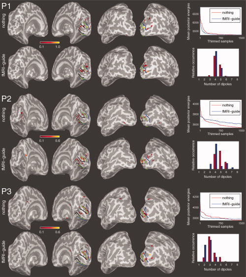
Left: Clustered locations of the chains from the drifting grating MEG experiment in subjects P1–P3 with and without fMRI‐guidance. Right: Mean posterior energies and number of sources in the clustered samples with and without fMRI‐guidance. [Color figure can be viewed in the online issue, which is available at www.interscience.wiley.com.]
The presented empirical results reveal more of the convergence properties of the sampler as well. Specifically, the convergence of the algorithm for subject P3, who clearly had the best SNR in the fMRI data, showed improvement in speed. Notably, the results for subject P2 are indecisive possibly due to poorer fMRI SNR and difficulties in the source space surface reconstruction related to acquiring the anatomical raw data with a 3 T magnet. With P1, the overall superb quality of his anatomical MRIs and good MEG SNR rendered the observed effect of improved convergence. On the basis of these observations it is presumable that the convergence is better for the fMRI‐guided case also with empirical data.
The relative occurences of number of dipoles in the clustered samples is similar in both cases. Regardless of clustered solution locations being quantitatively similar in both cases, the nonguided clustered locations are slightly more disperse, favoring the fMRI‐guided analysis. For example, with all the subjects (especially P2 and P3) the fMRI‐guide helped to get rid of some spurious dipole locations appearing on the left hemisphere without the fMRI‐guidance.
Despite being diffuse, the MEG inverse locations and different solution modes obtained with this approach coincide with the individual primary visual areas mapped with multifocal fMRI. Few example modes (i.e., solution estimates) of subjects P1 and P2 fMRI‐guided chains are displayed (see Fig. 10). Note that the estimation of the probability mass between the modes in here is impossible because the modes are from different chains and the sampler still has limited mixing properties between modes. Thus, one must rely on human expertise on interpreting which of the modes is the best given the underlying experimental task. For example, with subject P1 (chain 2), there is an early active dipole around 100 ms in V1 and later emerging dipoles close to V3/V3a of that individual. This is inline with the hypothesized activation pattern related to the drifting grating stimulus. Only in some of the chains such modes were visited that contained later emerging dipoles active in areas close to V5/MT. However, these dipoles were not shown in all the modes at the same location and did not show strong consistency. Along with the illustrated locations and latencies of the dipoles, a scatterplot depicting the datafit between forward calculated fields with original fields is shown. Just as in our previous study, the data fits are in general reasonable and equally good for different solution modes. The resulting solution modes of especially subjects P2 and P3 are not throughout as congruent with each other as is the case with the ones presented for subject P1.
Figure 10.

Representative example modes from four MCMC chains with fMRI‐guide are portrayed by estimated source locations, time courses, and datafit scatterplot of the forward calculated fields with respect to measured fields. [Color figure can be viewed in the online issue, which is available at www.interscience.wiley.com.]
DISCUSSION
Despite of many practical MEG inverse localization methods utilizing fMRI information are being available, the true nature of the coupling between the haemodynamic responses and electromagnetic measurements has not yet been revealed. In this study, we proposed a novel enhancement to a Bayesian, MCMC‐based, MEG inverse method in which fMRI data is used to construct a dipole location proposal distribution that guides the sampling algorithm. We validated the hypothesized improvements in the sampling efficiency by simulations and also tested the method with an empirical visual motion stimulus dataset, yielding a very complex inverse problem especially for an automated algorithm.
The simulation results suggest that the number of iterations required for plausible convergence with the fMRI‐guided sampler is smaller, if only clearly present in the simulated case (order of 3–5). Unfortunately, in the analyses of empirical data even the fMRI‐guided sampler seems to be hampered by poor mixing properties recognized already in our previous study without the fMRI information. However, the simulation results are encouraging and suggest that the localization accuracy and the dispersion of the dipole locations across different chains and modes are better with the fMRI‐guided method. Similar tendencies especially with the convergence properties of the sampler are observed also with the empirical results. Nonetheless, the multimodality makes it very difficult to properly obtain samples from the full posterior distribution and for the time being one must rely on, for instance, the clustered solutions presented in this study and to exemplars of representative solution modes. It is important to recall that one of the fundamental ideas in Bayesian MCMC‐based approaches is to aim at charting the whole distribution of possible solutions rather than one single estimate. In theory, this enables the researcher to commit himself on relating the experimental task with the activations rather than considering the confidence limits of the single point estimate first.
From the simulations, it seems evident that small errors in the fMRI‐guide (type I or II errors) do not seriously mislead the approach as long as the source is clearly detectable in MEG, that is the SNR is adequate. Conversely, the simulations suggest that in case of MEG source with low SNR, correct fMRI‐guidance is helpful. In fact, with the prevailing multimodality of the posterior distribution and deficiencies in the mixing capabilities of the sampler, the fMRI‐guide serves as a sort of implicit prior for the MEG inverse analysis although it is only used as a proposal distribution for the MCMC procedure. Importantly, this does not bias the results asymptotically even though the proposal distribution might not be accurate. This is desirable, since any suitable proposal distribution can then be used without invalidating the method. For instance, user defined seeding proposal distributions could be used, or even, in the absence of fMRI data, a beamformer style derived simple proposals from the MEG data alone. Such well‐grounded data‐driven MCMC methods have been used for example in image segmentation [Clark and Quinn,1999; Tu and Zhu,2002].
Another important virtue of our method is that with the two speed‐up strategies used [Auranen et al.,2007; Jun et al.,2005], the analysis of relatively long data segments (500 ms corresponding to roughly 150 timepoints) can be analyzed in a manageable time with current desktop computers. It is noteworthy, that with 204 MEG sensors and 100 timepoints, the required analysis time (for several MCMC chains) without the speed‐ups is in practice infeasible.
With experiments probing more complex aspects of, e.g., the visual or auditory system, it is convenient if the whole time course of the signal rather than just the peaks can be automatically analyzed. However, our approach still suffers from an obvious problem: the number of sources and their locations are required to stay fixed over the whole analysis period. Recently, Jun et al. [2006] presented an interesting modification to their original spatiotemporal dipole model which allows the source constellation to change over time. In their approach, activation starting and ending timepoints for each candidate source are added as additional unknown parameters in the analysis. These additional parameters are sampled as well and thus more realistic modeling of longer data sets is conceivable.
Although the inspection of the presented empirical data indicates that more accurate dipole fitting results might be achieved with traditional approaches, often requiring manual intervention and heuristic choices, the algorithm presented here serves as an alternative for fully automatic inverse analysis combining MEG/EEG and fMRI. It is possible that some preprocessing errors, such as imperfect coregistration of MEG and fMRI data, epi distortion, or noise in either data sets, reduce the efficiency of the experimental analyses. In spite of the multimodality of the posterior causing the sampler to operate perhaps more as a stochastic optimizer rather than an efficient sampler, there are clear advantages. The fMRI‐guided sampler can handle relatively large datasets, converges faster, is basically automatic, and, according to our simulations, yields better localization results than an approach based on MEG alone.
In conclusion, we demonstrated the benefits and possibilities of an automated fMRI‐guided MCMC‐based MEG inverse dipole localization method in a very challenging MEG inverse problem, which consisted of simulations and empirical MEG/fMRI data acquired during a presentation of a visual motion stimulus. In simulations, both the quantitative and qualitative localization accuracies are improved in comparison to the previous method without fMRI‐guidance for the MCMC sampler. With the empirical data, the dipoles are located at plausible sites in the low‐order visual areas and to some extent also at areas covering higher hierarchy in the human visual system indicating that these kind of methods can be utilized in evaluating the locations, latencies, and amplitudes of the combined fMRI and MEG brain activity.
Acknowledgements
The authors wish to thank M.D. Marja Balk for assistance in gathering the functional magnetic resonance imaging data.
REFERENCES
- Ahlfors SP,Simpson GV,Dale AM,Belliveau JW,Liu AK,Korvenoja A,Virtanen J,Huotilainen M,Tootell RBH,Aronen HJ,Ilmoniemi RJ ( 1999): Spatiotemporal activity of a cortical network for processing visual motion revealed by MEG and fMRI. J Neurophysiol 82: 2545–2555. [DOI] [PubMed] [Google Scholar]
- Auranen T,Nummenmaa A,Hämäläinen MS,Jääskeläinen IP,Lampinen J,Vehtari A,Sams M ( 2005): Bayesian analysis of the neuromagnetic inverse problem with lp‐norm priors. Neuroimage 26: 870–884. [DOI] [PubMed] [Google Scholar]
- Auranen T,Nummenmaa A,Hämäläinen MS,Jääskeläinen IP,Lampinen J,Vehtari A,Sams M ( 2007): Bayesian inverse analysis of neuromagnetic data using cortically constrained multiple dipoles. Hum Brain Mapp 28: 979–994. [DOI] [PMC free article] [PubMed] [Google Scholar]
- Baillet S,Garnero L ( 1997): A Bayesian approach to introducing anatomo‐functional priors in the EEG/MEG inverse problem. IEEE Trans Biomed Eng 44: 374–385. [DOI] [PubMed] [Google Scholar]
- Beckmann C,Jenkinson M,Smith SM ( 2003): General multi‐level linear modelling for group analysis in fMRI. Neuroimage 20: 1052–1063. [DOI] [PubMed] [Google Scholar]
- Belliveau JW,Kennedy DNJ,McKinstry RC,Buchbinder BR,Weisskoff RM,Cohen MS,Vevea JM,Brady TJ,Rosen BR ( 1991): Functional mapping of the human visual cortex by magnetic resonance imaging. Science 254: 716–719. [DOI] [PubMed] [Google Scholar]
- Bernardo JM,Smith AFM ( 1994): Bayesian Theory. Chichester: Wiley. [Google Scholar]
- Bertrand C,Ohmi M,Suzuki R,Kado H ( 2001): A probabilistic solution to the MEG inverse problem via MCMC methods: The reversible jump and parallel tempering algorithms. IEEE Trans Biomed Eng 48: 533–542. [DOI] [PubMed] [Google Scholar]
- Clark E,Quinn A ( 1999): A data‐driven Bayesian sampling scheme for unsupervised image segmentation. In: Proceedings of the IEEE International Conference on Acoustics,Speech, and Signal Processing, March 15–19, 1999, Phoenix, Arizona, USA.
- Courtney SM,Ungerleider LG ( 1997): What fMRI has taught us about human vision. Curr Opin Neurobiol 7: 554–561. [DOI] [PubMed] [Google Scholar]
- Dale AM,Fischl B,Sereno MI ( 1999): Cortical surface‐based analysis. I. Segmentation and surface reconstruction. Neuroimage 9: 179–194. [DOI] [PubMed] [Google Scholar]
- Dale AM,Liu AK,Fischl BR,Buckner RL,Belliveau JW,Lewine JD,Halgren E ( 2000): Dynamic statistical parametric mapping: Combining fMRI and MEG for high‐resolution imaging of cortical activity. Neuron 26: 55–67. [DOI] [PubMed] [Google Scholar]
- Daunizeau J,Grova C,Mattout J,Marrelec G,Clonda D,Goulard B,Pélégrini‐Issac M,Lina JM,Benali H ( 2005): Assessing the relevance of fMRI‐based prior in the EEG inverse problem: A Bayesian model comparison approach. IEEE Trans Signal Process 53: 3461–3472. [Google Scholar]
- DeYoe EA,Carman GJ,Bandettini P,Glickman S,Wieser J,Cox R,Miller D,Neitz J ( 1996): Mapping striate and extrastriate visusal areas in human cerebral cortex. Proc Natl Acad Sci USA 93: 2382–2386. [DOI] [PMC free article] [PubMed] [Google Scholar]
- Dougherty RF,Koch VM,Brewer AA,Fischer B,Modersitzki J,Wandell BA ( 2003): Visual field representations and locations of visual areas V1/2/3 in human visual cortex. J Vis 3: 586–598. [DOI] [PubMed] [Google Scholar]
- Engel SA,Glover GH,Wandell BA ( 1997): Retinotopic organization in human visual cortex and the spatial precision of functional MRI. Cereb Cortex 7: 181–192. [DOI] [PubMed] [Google Scholar]
- Fischl B,Liu A,Dale AM ( 2001): Automated manifold surgery: Constructing geometrically accurate and topologically correct models of the human cerebral cortex. IEEE Trans Med Imaging 20: 70–80. [DOI] [PubMed] [Google Scholar]
- Fischl B,Sereno MI,Dale AM ( 1999): Cortical surface‐based analysis II: Inflation, flattening, and a surface‐based coordinate system. Neuroimage 9: 195–207. [DOI] [PubMed] [Google Scholar]
- Friston KJ,Glaser DE,Henson RNA,Kiebel S,Phillips C,Ashburner J ( 2002a): Classical and Bayesian inference in neuroimaging: Applications. Neuroimage 16: 484–512. [DOI] [PubMed] [Google Scholar]
- Friston KJ,Penny W,Phillips C,Kiebel S,Hinton G,Ashburner J ( 2002b): Classical and Bayesian inference in neuroimaging: Theory. Neuroimage 16: 465–483. [DOI] [PubMed] [Google Scholar]
- Gelman A,Carlin JB,Stern HS,Rubin DB ( 2003): Bayesian Data Analysis, 2nd ed New York: Chapman and Hall. [Google Scholar]
- Gilks WR,Richardson S,Spiegelhalter DJ ( 1996): Markov chain Monte Carlo in Practice. New York: Chapman and Hall. [Google Scholar]
- Hämäläinen MS,Hari R,Ilmoniemi RJ,Knuutila J,Lounasmaa OV ( 1993): Magnetoencephalography—Theory, instrumentation, and applications to noninvasive studies of the working human brain. Rev Modern Phys 65: 413–497. [Google Scholar]
- Jenkinson M,Bannister P,Brady M,Smith S ( 2002): Improved optimisation for the robust and accurate linear registration and motion correction of brain images. Neuroimage 17: 825–841. [DOI] [PubMed] [Google Scholar]
- Jenkinson M,Smith SM ( 2001): A global optimisation method for robust affine registration of brain images. Med Image Anal 5: 143–156. [DOI] [PubMed] [Google Scholar]
- Jun SC,George JS,Paré‐Blagoev J,Plis SM,Ranken DM,Schmidt DM,Wood CC ( 2005): Spatiotemporal Bayesian inference dipole analysis for MEG neuroimaging data. Neuroimage 28: 84–98. [DOI] [PubMed] [Google Scholar]
- Jun SC,George JS,Plis SM,Ranken DM,Schmidt DM,Wood CC ( 2006): Improving source detection and separation in a spatiotemporal Bayesian inference dipole analysis. Phys Med Biol 51: 2395–2414. [DOI] [PubMed] [Google Scholar]
- Kaipio JP,Somersalo E ( 2005): Statistical and Computational Inverse Problems, Vol. 160 of Applied Mathematical Sciences. New York: Springer. [Google Scholar]
- Kincses WE,Braun C,Kaiser S,Grodd W,Ackermann H,Mathiak K ( 2003): Reconstruction of extended cortical sources for EEG and MEG based on a Monte‐Carlo‐Markov‐chain estimator. Hum Brain Mapp 18: 100–110. [DOI] [PMC free article] [PubMed] [Google Scholar]
- Korvenoja A,Huttunen J,Salli E,Pohjonen H,Martinkauppi S,Palva JM,Lauronen L,Virtanen J,Ilmoniemi RJ,Aronen HJ ( 1999): Activation of multiple cortical areas in response to somatosensory stimulation: Combined magnetoencephalographic and functional magnetic resonance imaging. Hum Brain Mapp 8: 13–27. [DOI] [PMC free article] [PubMed] [Google Scholar]
- Kwong KK,Belliveau JW,Chesler DA,Goldberg IE,Weisskoff RM,Poncelet BP,Kennedy DN,Hoppel BE,Cohen MS,Turner R,Cheng HM,Brady TJ,Rosen BR ( 1992): Dynamic magnetic resonance imaging of human brain activity during primary sensory stimulation. Proc Natl Acad Sci USA 89: 5675–5679. [DOI] [PMC free article] [PubMed] [Google Scholar]
- Liu AK,Belliveau JW,Dale AM ( 1998): Spatiotemporal imaging of human brain activity using functional MRI constrained magnetoencephalography data: Monte Carlo simulations. Proc Natl Acad Sci USA 95: 8945–8950. [DOI] [PMC free article] [PubMed] [Google Scholar]
- Mosher JC,Leahy RM,Lewis PS ( 1999): EEG and MEG: Forward solutions for inverse methods. IEEE Trans Biomed Eng 46: 245–259. [DOI] [PubMed] [Google Scholar]
- Nunez PL ( 1981): Electric Fields of the Brain: The Neurophysics of EEG. New York: Oxford University Press. [Google Scholar]
- Ogawa S,Tank DW,Menon R,Ellermann JM,Kim S,Merkle H,Ugurbil K ( 1992): Intrinsic signal changes accompanying sensory stimulation: Functional brain mapping with magnetic resonance imaging. Proc Natl Acad Sci USA 89: 5951–5955. [DOI] [PMC free article] [PubMed] [Google Scholar]
- Phillips C,Mattout J,Rugg MD,Maquet P,Friston KJ ( 2005): An empirical Bayesian to the source reconstruction problem in EEG. Neuroimage 24: 997–1011. [DOI] [PubMed] [Google Scholar]
- Phillips JW,Leahy RM,Mosher JC ( 1997): MEG‐based imaging of focal neuronal current sources. IEEE Trans Med Imaging 16: 338–348. [DOI] [PubMed] [Google Scholar]
- Sarvas J ( 1987): Basic mathematical and electromagnetic concepts of the biomagnetic inverse problem. Phys Med Biol 32: 11–22. [DOI] [PubMed] [Google Scholar]
- Schmidt DM,George JS,Ranken DM,Wood CC ( 2000): Spatial‐temporal Bayesian inference for MEG/EEG. In: Biomag 2000: 12th International Conference on Biomagnetism,Espoo, Finland. URL http://biomag2000.hut.fi/papers/0671.pdf.
- Schmidt DM,George JS,Wood CC ( 1999): Bayesian inference applied to the electromagnetic inverse problem. Hum Brain Mapp 7: 195–212. [DOI] [PMC free article] [PubMed] [Google Scholar]
- Sereno MI,Dale AM,Reppas JB,Kwong KK,Belliveau JW,Brady TJ,Rosen BR,Tootell RBH ( 1995): Borders of multiple visual areas in humans revealed by functional magnetic resonance imaging. Science 268: 889–893. [DOI] [PubMed] [Google Scholar]
- Smith SM,Jenkinson M,Woolrich MW,Beckmann CF,Behrens TEJ,Johansen‐Berg H,Bannister PR,Luca MD,Drobnjak I,Flitney DE,Niazy RK,Saunders J,Vickers J,Zhang Y,Stefano ND,Brady JM,Matthews PM ( 2004): Advances in functional and structural MR image analysis and implementation as FSL. Neuroimage 23: S208–S219. [DOI] [PubMed] [Google Scholar]
- Tu Z,Zhu SC ( 2002): Image segmentation by data‐driven Markov chain Monte Carlo. IEEE Trans Pattern Anal Mach Intell 24: 657–673. [Google Scholar]
- Vanni S,Dojat M,Warnking J,Delon‐Martin C,Segebarth C,Bullier J ( 2004a): Timing of interactions across the visual field in the human cortex. Neuroimage 21: 818–828. [DOI] [PubMed] [Google Scholar]
- Vanni S,Henriksson L,James AC ( 2005): Multifocal fMRI mapping of visual cortical areas. Neuroimage 27: 95–105. [DOI] [PubMed] [Google Scholar]
- Vanni S,Warnking J,Dojat M,Delon‐Martin C,Bullier J,Segebarth C ( 2004b): Sequence of pattern onset responses in the human visual areas: An fMRI constrained VEP source analysis. Neuroimage 21: 801–817. [DOI] [PubMed] [Google Scholar]
- Watson JDG,Myers R,Frackowiak RSJ,Hajnal JV,Woods RP,Mazziotta JC,Shipp S,Zeki S ( 1993): Area V5 of the human brain: Evidence from a combined study using positron emission tomography and magnetic resonance imaging. Cereb Cortex 3: 79–94. [DOI] [PubMed] [Google Scholar]
- Woolrich MW,Behrens TEJ,Beckmann CF,Jenkinson M,Smith SM ( 2004): Multi‐level linear modelling for fMRI group analysis using Bayesian inference. Neuroimage 21: 1732–1747. [DOI] [PubMed] [Google Scholar]
- Woolrich MW,Ripley BD,Brady JM,Smith SM ( 2001): Temporal autocorrelation in univariate linear modelling of fMRI data. Neuroimage 14: 1370–1386. [DOI] [PubMed] [Google Scholar]
- Worsley KJ,Evans AC,Marrett S,Neelin P ( 1992): A three‐dimensional statistical analysis for CBF activation studies in human brain. J Cereb Blood Flow Metab 12: 900–918. [DOI] [PubMed] [Google Scholar]