

Abstract
This article reviews progress and challenges in model driven EEG/fMRI fusion with a focus on brain oscillations. Fusion is the combination of both imaging modalities based on a cascade of forward models from ensemble of post‐synaptic potentials (ePSP) to net primary current densities (nPCD) to EEG; and from ePSP to vasomotor feed forward signal (VFFSS) to BOLD. In absence of a model, data driven fusion creates maps of correlations between EEG and BOLD or between estimates of nPCD and VFFS. A consistent finding has been that of positive correlations between EEG alpha power and BOLD in both frontal cortices and thalamus and of negative ones for the occipital region. For model driven fusion we formulate a neural mass EEG/fMRI model coupled to a metabolic hemodynamic model. For exploratory simulations we show that the Local Linearization (LL) method for integrating stochastic differential equations is appropriate for highly nonlinear dynamics. It has been successfully applied to small and medium sized networks, reproducing the described EEG/BOLD correlations. A new LL‐algebraic method allows simulations with hundreds of thousands of neural populations, with connectivities and conduction delays estimated from diffusion weighted MRI. For parameter and state estimation, Kalman filtering combined with the LL method estimates the innovations or prediction errors. From these the likelihood of models given data are obtained. The LL‐innovation estimation method has been already applied to small and medium scale models. With improved Bayesian computations the practical estimation of very large scale EEG/fMRI models shall soon be possible. Hum Brain Mapp, 2009. © 2008 Wiley‐Liss, Inc.
Keywords: alpha rhythm, EEG, fMRI, oscillation, neural mass models, hemodynamic response
INTRODUCTION
The principled combination of information from both modalities to achieve images with simultaneously high spatial and temporal resolution is what we shall term EEG/fMRI fusion [Ritter and Villringer, 2006]. It can be either data driven or model driven (see Fig. 1). Although data driven fusion provides empirical constraints for modeling, it is model driven fusion that will provide deeper understanding of neural mechanisms. This article shall review progress and challenges in analyzing brain oscillations with model driven EEG/fMRI fusion. Some recent methodological advances will also be highlighted. At the onset, we state that we limit our analysis to resting state oscillatory brain activity due, not only to space limitations, but also because there is a consistent body of work in this area that can also provide insight into the analysis of evoked and induced activity. When relevant we will include information on models with steady state stimulation. Another advantage of limiting our attention to resting state activity is that here we sidestep the mismatch in temporal resolution between EEG and fMRI, only occupying our attention with slow variations in the parameters of the resting state.
Figure 1.
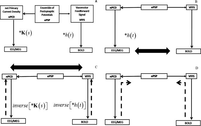
Strategies for EEG/fMRI data analysis. A: Simplified underlying forward models (FMs) for fusion. In a given voxel neural activity generates an ensemble of postsynaptic potentials (ePSP). Along the left branch of the diagram the temporally and spatially synchronized summated PSPs of neurons with open fields produce the primary current density (PCD). This is the PCD FM. The volume conductor properties of the head transform the PCD into EEG/MEG which is the FM for this type of signal. Along the right branch of this diagram, the ePSP generates a vasomotor feed forward signal (VFFS) via its own FM, which in turn is transformed via the hemodynamic FM into the observed BOLD signal. Note that any one of the model constructs enumerated here (ePSP, PCD, VFFS, EEG/MEG, BOLD) is time dependent and, according to the type of modeling, can be defined as either a single variable or a vector of variables. B: Fusion by measuring covariation of the EEG and BOLD. In this data driven approach to EEG/fMRI fusion the EEG is considered to have the same time evolutin as the PCD which is considered as a driver for the BOLD signal. The time varying power in an EEG band is convolved with a hemodynamic response function, h(t), and then correlated with the BOLD signal (correlation denoted by a thick arrow). Since the temporal dynamics of the EEG are taken as a surrogate for the VFFS this is an asymmetrical type of fusion. C: Fusion by measuring co‐variation of the PCD and VFFS. This is also a data driven approach in which the FMs for the EEG/MEG and BOLD are inverted, by solving respectively a spatial and temporal inverse problem to yield estimates of the PCD and VFFS. These estimates are then correlated (thick arrow) to accomplish a fusion that is symmetrical in that both modalities are given equal a priori weight. D: Model Driven Fusion by estimating the ePSP from EEG and BOLD. This is a model driven approach in which simultaneous Bayesian inversion is carried out with all FMs. In practice this involves repeated simulations with tentative values of ePSPs and other parameters and then modifying them to maximize an statistical measure of fit. One possible method for this estimation is shown in Figure 4.
Nevertheless the theoretical interpretation of this type of activity is of great importance. Oscillatory brain activity seems to be the weft that holds together the fabric of neural computations [Varela et al., 2001]. Several types of resting state and evoked rhythmic activity have been observed in local field potential (LFP)[Engel et al., 2001], electro and magneto‐encephalographic activity (EEG/MEG)[Buzsaki and Draguhn, 2004] as well as, more recently, in recordings of blood‐oxygen‐level dependent signals (fMRI)[Fox and Raichle, 2007]. These rhythmic activities have been found to be signatures of different behavioral states. The concurrent measurement of both the EEG and fMRI [Ives et al., 1993; Laufs et al., 2008] and the emergence of EEG/fMRI fusion methods promises improved identification of the neural ensembles—and the connections between them—that generate these different brain rhythms [Goldman et al., 2002].
Regarding EEG/fMRI fusion methods, are all based on the conceptual framework shown in Figure 1A. It is assumed that neural activity is transformed into recorded EEG or BOLD signal by corresponding forward models. We simplify current knowledge by assuming that the ensemble of postsynaptic potentials (ePSP) of neurons at a given voxel is the main contributor to both types of recordings [Attwell Iadecola, 2002; Logothetis, 2002; Riera et al., 2008]. To arrive at the EEG, a first forward model summarizes ePSPs from neurons with the appropriate geometry, spatial arrangement and temporal synchronization resulting in a net primary current density (PCD) distribution. This, in turn, is subject to a second transformation, a linear spatial convolution with the EEG Lead Field [Nunez and Silberstein, 2000]. The pathway to the BOLD signal also comprises two transformations, one which transforms the ePSPs into a local Vasomotor feed forward signal (VFFS) that then undergoes a (possibly nonlinear) temporal convolution with the hemodynamic response function (hrf). Usual inference from the data to the unobserved quantities proceeds in isolation along each branch solving the following inverse problems:
Estimating the PCD from EEG/MEG–the EEG (spatial) inverse problem [Trujillo‐Barreto et al., 2004]
Estimating the VFFS from the BOLD‐fMRI deconvolution or (temporal) inverse problem [Glover, 1999]
In contrast, EEG/fMRI fusion involves combining information (either observed data or estimated constructs) from both of the two cascades of forward models shown in Figure 1A. Fusion methods may be classified according to two criteria:
-
1
Asymmetrical versus symmetrical fusion: If one modality is given privileged status as a prior for the other modality we shall call this “asymmetrical fusion.” For example if BOLD activation is used as a spatial constraint for EEG sources [Liu et al., 1998]. By contrast “symmetrical approaches” do not assign an a priori inferential preference to any given modality [Trujillo‐Barreto et al., 2001]. In symmetrical fusion the best of each modality will be exploited and their relative importance determined from the data [Daunizeau et al., 2007].
-
2
Data versus model driven fusion: A further distinction is that of data driven fusion which is based on measuring mutual dependence between the two modalities in contrast to model driven fusion which exploits models of the chain of events leading to observed measurements. More specifically, the aim is to estimate the ePSP from both either the PCD or the VFFS. In terms of a widely used distinction [Friston, 1994] data driven approaches establish functional connectivities between observables/constructs while model driven approaches establish effective connectivity between them.
We now describe in more detail data driven EEG/fMRI fusion of resting state oscillatory activity that serves as a constraint for model driven efforts. For convenience of the reader a list of terms used in this article and their abbreviations are presented in Table I.
Table 1.
List of the abbreviations used in the paper
| Abbreviation | Meaning |
|---|---|
| ACP | Anatomical Connection Probability |
| BOLD | Blood Oxygenation Level Dependent |
| CBF | Cerebral Blood Flow |
| DCM | Dynamic causal model |
| DWMRI | Diffusion weighted magnetic resonance imaging |
| EEG | Electroencephalogram |
| ePSP | Ensemble of post‐synaptic potentials |
| EPSP | Excitatory post synaptic potential |
| fMRI | Functional magnetic resonance imaging |
| fdr | False discovery rate |
| hrf | Hemodynamic Response Function |
| Inh | Inhibitory interneurons |
| IPSP | Inhibitory post synaptic potential |
| LL | Local linearization |
| LRC | Long range connections |
| MHM | Metabolic/hemodynamic model |
| ODE | Ordinary Differential Equation |
| PCD | Primary current density |
| PSP | Post‐synaptic potentials |
| Pyr | Pyramidal cells |
| RDE | Random differential equations |
| RE | thalamic inhibitory reticular neurons |
| SDE | Stochastic differential equations |
| SRC | Short range connections |
| SSM | State‐space models |
| St | Stellate cells |
| TC | thalamocortical excitatory relay neurons |
| VFSS | Vasomotor feed‐fodward signal |
CONSTRAINTS PROVIDED BY DATA DRIVEN FUSION
Most work on data driven EEG/fMRI fusion of resting state rhythms has mapped measures of association or correlation of the EEG signal and BOLD as schematized in Figure 1C. According to our classification it has been of the asymmetrical fusion type, the EEG serving as a surrogate for the VFFS (Fig. 1A). Towards this end, estimates of power in specific spectral bands are summarized over certain EEG channels, convolved with a standard hemodynamic response function, and then correlated with the BOLD time course at each voxel. The resulting image is then thresholded to produce a SPM map of EEG‐BOLD correlation. Goldman et al. [2002] found positive alpha band/BOLD correlations in the thalamus and negative ones in the occipital cortex, somatosensory areas and the insula. Such findings have been replicated and extended by several other authors as nicely reviewed by Laufs [Laufs, 2008]. The initial findings were obtained with single EEG frequency band, alpha, averaged over posterior leads. This univariate approach is open to the criticism that the observed correlations with BOLD might actually be due to other, unobserved EEG frequency bands. This problem was remedied by multiple regressions of the BOLD on all EEG frequency bands [Laufs et al., 2003; Mantini et al., 2007]. This procedure highlighted the relation of the β2 band with the “default” fMRI resting state mode. An even more comprehensive approach is that of [Martinez‐Montes et al., 2004] who carried out EEG/fMRI fusion of the original Goldman et al. data set by a structured combination of spatial, temporal and frequency information of the EEG via a multilinear version of partial least squares. This method recognizes that a multichannel EEG time varying spectrum is a 3 dimensional array indexed by channel, frequency and time that can be decomposed into a sum of EEG “atoms” which each have a given spatial, spectral and temporal signature. The way these atoms are extracted ensures maximal covariance of their temporal signatures with those of BOLD atoms (with time and spatial signatures). Figure 2A shows the inverse solution of the EEG alpha atom spatial signature [Bosch‐Bayard et al., 2001] and the fMRI alpha spatial signature with a significant correlation that is positive for the thalamus and negative for cortical areas. It also shows that the EEG sources that mainly contribute to these correlations are concentrated in the occipital areas. The pattern has been speculated to be due to desynchronization of EEG generators with fluctuations to higher levels of vigilance and lower alpha power a conclusion reinforced by the experimental manipulation of these atoms by switching the subject from a resting state to mental arithmetic [Miwakeichi et al., 2004].
Figure 2.
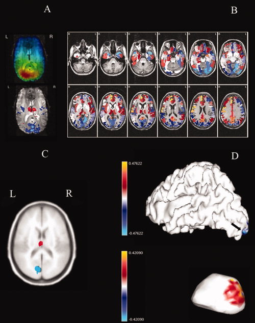
(Color) A: Fusion by correlation of EEG time varying spectra over all channels and BOLD. Data driven asymmetrical fusion as in Figure 1b where EEG spectra convolved with hemodynamic response function is correlated with BOLD signal using multi‐linear partial least squares which detects common atoms in both modalities. Top: Spatial signatures of PCD for the EEG alpha atom estimated by f inverse solution. Bottom: spatial signature of BOLD alpha atom. B: Fusion by correlation of log PCD alpha power and log VFFS. Symmetrical data driven EEEG/fMRI fusion as in Figure 1c obtained by estimating the time course of EEG source power in the alpha band using the VARETA inverse solution, estimating the VFFS by smooth deconvolution of the BOLD signal with a standard hemodynamic response, and correlating the log of these quantities at each voxel. C: Correlation of source EEG and BOLD in neural mass network of moderate size. Correlation of estimated PCDs and VFFS obtained from a medium sized simulation of realistically connected neural masses. Connectivity measures for neural masses were estimated by means of DTI images. Correlation values threshold using the local false discovery rate (fdr). Red corresponds to positive correlations, blue to negative correlations. Simulations produced by the Local Linearization (LL) integration scheme for stochastic differential equations. D: Correlation of source EEG and BOLD in large scale neural mass network (surface of cortex and thalamus. Correlation of estimated PCDs and VFFS obtained from a very large sized simulation of realistically connected neural masses. Correlations shown for the cortical surface (above) and the thalamus (below not shown to scale) with the rostral part shown to the left. The cortical surface comprised 8203 Jansen modules were placed) and the left portion of the thalamus 438 TC/RT modules. The simulation produced (not shown) similar distributions for the right brain. All modules interconnected using the connectivity matrix shown in Figure 5. Note positive (red) PCD/BOLD correlation for caudal thalamus and negative (blue) for part of the occipital cortex marked by an arrow. Simulations produced by the approximae Local Linearization (aLL) integration scheme for stochastic differential equations.
Data driven methods for EEG/fMRI fusion of brain oscillations can be further improved. We now give a example. As mentioned these methods are asymmetrical in the sense that the EEG is taken as a surrogate for the VFFS but this involves degrading the temporal resolution of the EEG signal by filtering with a low pass signal (the hrf). A higher resolution, symmetrical, data driven fusion can be gained by measuring the correlation between estimates of the PCD and VFFS instead of using the usual correlation between the hrf filtered EEG and BOLD. Results from a 96 channel concurrent EEG/fMRI recording of the resting state are shown in Figure 2B. The estimate of power at the alpha peak of the nPCD was obtained by means of the VARETA inverse solution [Bosch‐Bayard et al., 2001]. The VFFS at each voxel was obtained by a spline variant of BOLD deconvolution (Appendix A). We found more widespread correlations with nPCD/VFFS fusion than with EEG/BOLD fusion, the pattern here being thalamic and anterior cortical areas directly related and posterior cortical areas inversely related to alpha power. It should also be pointed out that much higher correlations (range −0.73 to 0.52) were found when comparing the logarithms of PCD and VFFS than when comparing EEG and BOLD (range −0.54 to 0.41).
Thus a consistent pattern for resting state EEG/fMRI relations has been described by a number of authors. We now turn to model driven EEG/fMRI fusion methods to see if these patterns can be explained.
MODEL DRIVEN EEG/fmri FUSION: STATE SPACE MODELS
Model driven EEG/fMRI fusion is predicated on the formulation of explicit biophysical model for the two different chains of forward events (Fig. 1A) that lead from the ePSP to the EEG, on the one hand, and to BOLD on the other. Once these models are formulated it is possible to:
Simulate EEG and fMRI signals originated by neural activity and study their interrelation
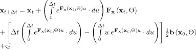
Given data, estimate neural activity—the ePSP—as well as other model parameters (Figs. 1D and 4).
Figure 4.
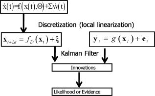
Local linearization (LL)‐innovation approach to estimating states and parameters of nonlinear random systems. A state space model of a dynamical system is the combination of: (a) A continuous time stochastic differential equation describing the evolution of system states x, and (b) A discrete time observation equation that explains how the observations y t are obtained from the states. Discretization of the state equation by means of the Local Linearization scheme allows the application of sequential Bayesian inference of the unobserved states via the Kalman Filter. This in turn allows the estimation of the innovations or prediction error which in turn can be used to estimate the likelihood of the model. Once the likelihood has been obtained estimation of model parameters and comparison of models is possible.
EEG/fMRI models are particular cases of State Space Models (SSM)[Kalman, 1960]1
| (1) |
The first line expresses the state equation, a set of stochastic differential equations (SDE) that describe how the state vector x(t) of the system evolves in continuous time. The vector v(t) describes external inputs, controls or causes that influence the system. The set of parameters specifying the model is Θ. The vector  contains the dynamic noise, random inputs to the system that are modeled as a Gaussian white noise process2. μ is the mean of the random input and Σ is a square root of a covariance matrix. The second equation, the observation equation, describes how the observations y
t are determined by the states x
t = x(t) at discrete time instants t, and corrupted by measurement noise e
t. SSM are well known in control theory since the 1960s [Frost and Kailath, 1971; Kalman, 1960].
contains the dynamic noise, random inputs to the system that are modeled as a Gaussian white noise process2. μ is the mean of the random input and Σ is a square root of a covariance matrix. The second equation, the observation equation, describes how the observations y
t are determined by the states x
t = x(t) at discrete time instants t, and corrupted by measurement noise e
t. SSM are well known in control theory since the 1960s [Frost and Kailath, 1971; Kalman, 1960].
In the neuroimaging literature SSM have become popular under the name Dynamic Causal Models (DCM) [Friston et al., 2003]. The initial formulation of DCM [Friston et al., 2003] did not consider noise inputs (Σ = 0) and was therefore a deterministic SSM stated in terms of ordinary differential equations (ODE). More recent versions have been in terms of SDEs [Chen et al., 2008; Friston et al., 2008; Stephan et al., 2008]. We note that since the focus of this article is EEG/fMRI fusion of resting state oscillations, we shall not consider in the remainder of this article the external inputs v(t) in Eq. (1). SSM (DCM) with external inputs v(t) are of course necessary for studying event related [(David et al., 2006b, c; Friston, 2006]) or induced activity [Chen et al., 2008].
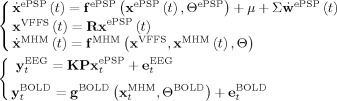
Mapping the EEG/fMRI generative model of Figure 1A onto a SSM we define:
x ePSP are the state variables that define the evolution of ePSP according to some neural model.
P is a projection matrix that selects and sums thosecomponents of the ePSP that contribute to the PCD.
K is the lead field matrix that projects the PCD to an observed EEG/MEG measurement.
R is the projection matrix that transforms x ePSP into the VFFS x VFFS;
 are the state variables that together with x
VFFS define the evolution of a metabolic hemodynamic model (MHM) [Sotero and Trujillo‐Barreto, 2007, 2008].
are the state variables that together with x
VFFS define the evolution of a metabolic hemodynamic model (MHM) [Sotero and Trujillo‐Barreto, 2007, 2008].g BOLD is the model that relates the MHM model to the observed BOLD signal.
y and y are the discretized EEG and BOLD measurements respectively.
The particular form of SSM that underlies model driven EEG/fMRI fusion (Fig. 1D) is then
 |
(2) |
In these equations state variables, functions, dynamic noises, measurement noises and parameters all are labeled with corresponding superscripts that describe the part of Figure 1A they refer to. Note that we have assumed a deterministic model for the MHM though this can be generalized to a stochastic model with dynamic noise [Sotero et al., 2008].
Models f ePSP for describing the evolution of ePSPs (at the root of Fig. 1A) can be constructed at various levels of detail. Recent examples [Izhikevich and Edelman, 2008] have incorporated comprehensive information about the microcircuitry [Riera et al., 2008] of the brain. We shall focus rather on a mesoscopic level more suited to the coarse grained nature of both EEG and fMRI measurements. These are the class of neural mass models for EEG oscillators [David and Friston, 2003; Jansen and Rit, 1995; Lopes da Silva et al., 1974; Moran et al., 2007; Valdes et al, 1999a, b ; Wilson and Cowan, 1972] obtained by mean field approximations of subpopulations of excitatory and inhibitory neurons each governed by well known dynamics. See [David et al., 2006a; Harrison et al., 2006] for a review on how to obtain these equations. We shall now specify these mesoscopic models in a format slightly different from the cited references.
Consider i = 1,…,N m neural mass models that give rise to the state vector x ePSP, these are chosen to correspond to a discretization of the brain that can be as coarse as the grid for estimating nPCD, BOLD or even finer. Each neural mass x is cast as a noisy oscillator (Fig. 3A)
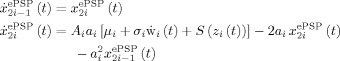 |
(3) |
Figure 3.
Neural Mass model for EEG/fMRI fusion. This model is obtained by linking the parameters of a interconnected set of N
m neural masses to the forward models for EEG and fMRI outlined in figure 1A where averaged population values of postsynaptic potentials (PSP) serve as state variables. A: State Space Model (SSM) for a Neural Mass. Each Neural Mass (numbered as i) is shown on the right part of the figure and depicted as a component which receives two external inputs: the net input PSP z
i(t) (continuous arrow), and Gaussian white noise  (dashed arrow). The neural mass produces as an output the ePSPs x
which are also the state variables for this SSM. The ePSPs will feed into other neural masses. Note that z
i(t) is the sum of the ePSPs that are emitted from other connected neural masses, amplified by the synaptic contact coefficients z
i(t) = ∑
c
i,j
x
2j−1(t), where c
i,j indicates connections from population j to i. By convention these synaptic connectivities will be negative for when j is an inhibitory cell. On the left is shown in more detail the sequence of operations which take input to output: 1 − z
i(t) is converted into an average pulse density of action potentials p
i(t) = S(z
i(t)) by a static nonlinear sigmoid function S(v). 2‐The noise input, with mean μi and standard deviation σi, is added to the pulse density. 3 ‐
(dashed arrow). The neural mass produces as an output the ePSPs x
which are also the state variables for this SSM. The ePSPs will feed into other neural masses. Note that z
i(t) is the sum of the ePSPs that are emitted from other connected neural masses, amplified by the synaptic contact coefficients z
i(t) = ∑
c
i,j
x
2j−1(t), where c
i,j indicates connections from population j to i. By convention these synaptic connectivities will be negative for when j is an inhibitory cell. On the left is shown in more detail the sequence of operations which take input to output: 1 − z
i(t) is converted into an average pulse density of action potentials p
i(t) = S(z
i(t)) by a static nonlinear sigmoid function S(v). 2‐The noise input, with mean μi and standard deviation σi, is added to the pulse density. 3 ‐  is converted into the output x
(t) by linear convolutions with the neural PSP impulse responses h
i(t). The complete neural mass model creates two additional signals (not shown) that will act as the two components of the VFSS signal originating the BOLD signal. These are the sum of all EPSP u
E(t) = ∑
c
i,j
x2j−1(t) and all IPSP u
I(t) = −∑
c
i,j
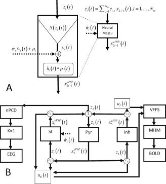
x2j−1(t). B: Model for a Jansen‐Rit Cortical Module. Here N
m = 3. Pyramidal cell (Pyr), stellate cell (St), and inhibitory interneuron (Inh) populations generate ePSPs, denoted respectively by {x
(t), x
(t), x
(t)}. The output of Pyr cells, x
(t), multiplied by c
1,2, c
3,2 drives the St and Inh populations. Pyr receives feedback from St and Inh with coefficients c
2,1, c
2,3 respectively. The only dynamic noise input is to the St Population. On the one hand, the nPCD is the transmembrane PSP of the Pyr population which is equal to the net input PSP z
2(t) generated by the St and Inh populations z
2(t) = c
2,1
x
(t) + c
2,3
x
(t) (EPSP‐IPSP). This is also equal to the EEG with the trivial lead field K = 1. Loosely speaking, this is as though we were actually measuring a Local Field Potential (LFP). On the other hand, The VFFS has two components
is converted into the output x
(t) by linear convolutions with the neural PSP impulse responses h
i(t). The complete neural mass model creates two additional signals (not shown) that will act as the two components of the VFSS signal originating the BOLD signal. These are the sum of all EPSP u
E(t) = ∑
c
i,j
x2j−1(t) and all IPSP u
I(t) = −∑
c
i,j
x2j−1(t). B: Model for a Jansen‐Rit Cortical Module. Here N
m = 3. Pyramidal cell (Pyr), stellate cell (St), and inhibitory interneuron (Inh) populations generate ePSPs, denoted respectively by {x
(t), x
(t), x
(t)}. The output of Pyr cells, x
(t), multiplied by c
1,2, c
3,2 drives the St and Inh populations. Pyr receives feedback from St and Inh with coefficients c
2,1, c
2,3 respectively. The only dynamic noise input is to the St Population. On the one hand, the nPCD is the transmembrane PSP of the Pyr population which is equal to the net input PSP z
2(t) generated by the St and Inh populations z
2(t) = c
2,1
x
(t) + c
2,3
x
(t) (EPSP‐IPSP). This is also equal to the EEG with the trivial lead field K = 1. Loosely speaking, this is as though we were actually measuring a Local Field Potential (LFP). On the other hand, The VFFS has two components  , the sum of excitatory PSP and u
I(t) = c
2,3
x
(t) the inhibitory PSP. The VFSS components are fed into the Metabolic Hemodynamic Model (MHM) which we shall not detail here (see Appendix C) a system of ODE which depends on additional state variables x
7(t),…,x
14(t). The observed BOLD is generated by the Balloon model then is transformed to BOLD by the equation y
2(t) = g
BOLD (x
13(t),x
14(t)).
, the sum of excitatory PSP and u
I(t) = c
2,3
x
(t) the inhibitory PSP. The VFSS components are fed into the Metabolic Hemodynamic Model (MHM) which we shall not detail here (see Appendix C) a system of ODE which depends on additional state variables x
7(t),…,x
14(t). The observed BOLD is generated by the Balloon model then is transformed to BOLD by the equation y
2(t) = g
BOLD (x
13(t),x
14(t)).
The variable x
(t) is the average output ePSP produced by each neural mass which can be either excitatory (EPSP) or inhibitory (IPSP) while  is its time derivative. The variables x
(t) are the transformation of the net input to the mass z
i(t) by the application of first a nonlinear sigmoid function S(z
i(t)) and then a linear convolution with the neural PSP impulse response functions h
i(t). The Laplace transform of h
i(t) originates the second order ODE. Note that dynamic noise
is its time derivative. The variables x
(t) are the transformation of the net input to the mass z
i(t) by the application of first a nonlinear sigmoid function S(z
i(t)) and then a linear convolution with the neural PSP impulse response functions h
i(t). The Laplace transform of h
i(t) originates the second order ODE. Note that dynamic noise  may be added to S(z
i(t)) transforming (3) into a SDE.
may be added to S(z
i(t)) transforming (3) into a SDE.
The sigmoid function is defined [David et al., 2006a] as  , where 2e
0 is the maximum firing rate, v
0 is the postsynaptic potential (PSP) corresponding to a firing rate e
0, and parameter r controls the steepness of the sigmoid function S(z
i(t)). These sigmoid function parameters are usually fixed. The impulse responses are defined as h
i(t) = A
i
a
i
te
where the parameter A
i represents the maximum amplitude of the EPSP or IPSP, while the lumped parameters a
i depends on passive membrane time constants and other distributed delays in the dendritic network. Note that these constants differ for excitatory and the inhibitory neural masses respectively, though they are usually considered constant for whole groups of neural masses (see Appendix B for typical parameter values).
, where 2e
0 is the maximum firing rate, v
0 is the postsynaptic potential (PSP) corresponding to a firing rate e
0, and parameter r controls the steepness of the sigmoid function S(z
i(t)). These sigmoid function parameters are usually fixed. The impulse responses are defined as h
i(t) = A
i
a
i
te
where the parameter A
i represents the maximum amplitude of the EPSP or IPSP, while the lumped parameters a
i depends on passive membrane time constants and other distributed delays in the dendritic network. Note that these constants differ for excitatory and the inhibitory neural masses respectively, though they are usually considered constant for whole groups of neural masses (see Appendix B for typical parameter values).
A Neural Mass model is the interconnection of several neural masses. The ePSPs x
(t) produced by each component population will feed into other neural masses. Note that z
i(t) is the sum of the ePSPs that are emitted from other connected neural masses, amplified by the synaptic contact coefficients  , where C = {c
i,j} indicates synaptic strengths of connections from neural mass j to neural mass i. By convention these synaptic connectivities will be negative when j is an inhibitory cell. These relations are summarized by:
, where C = {c
i,j} indicates synaptic strengths of connections from neural mass j to neural mass i. By convention these synaptic connectivities will be negative when j is an inhibitory cell. These relations are summarized by:
| (4) |
In correspondence with the general EEG/fMRI SMM (2) the recorded EEG is
 |
(5) |
in which expression several things have happened
x ePSP(t), and therefore z(t) has been discretized (see the next section on correct ways of doing this).
Of all z t only those corresponding to neural populations with open fields [Nunez et al., 2000, 2001] will contribute to the nPCD, as selected by the matrix P open which also determines the level of spatial averaging we shall select for the primary current.
The EEG is obtained by projection to the lead field and addition of sensor noise.
Both EPSP and IPSP may contribute to the BOLD signal [Sotero and Trujillo‐Barreto, 2007, 2008; Sotero et al., 2008; Riera et al., 2006; Babajani and Soltanian‐Zadeh, 2006; Babajani et al., 2005]. We will therefore consider additional variables that form part of the VFSS vector. These are the sum of all EPSP u E(t) and all IPSP u I(t) in a volume generating the BOLD signal
 |
(6) |
Generation of the BOLD signal proceeds then according to Appendix C
With this formalism in place we can discuss the different models, of every increasing complexity, have been dealt with in the literature. We shall classify these models into small scale, medium scale, and large scale models according to the ability to deal with hundreds, thousands and hundreds of thousands of neural masses.
SIMULATION OF STATE SPACE MODELS
We shall now review methods for simulations of SSM. These simulations are useful for two reasons. In the first place inspection of the simulated time series and comparison with actual data can provide face validity for the models being proposed. Moreover bifurcations of the modeled nonlinear systems with changes in parameter values suggest neural mechanisms of normal and abnormal brain activity [Lopes da Silva et al., 2003; Breakspear et al., 2006; Coombes et al., 2007]. In the second place, as will be argued in the next section, repeated simulations are the basis for the estimation of states and parameters.
Simulation consists of integrating the system of SDE (1) which, for interesting nonlinear cases, cannot be done analytically. Therefore it is customary to find either:
global approximations that allow analytical solutions for theoretical work [Moran et al., 2007] or
local approximations in order to calculate numerical values of the state vector x = x(t k) for time steps t k = k Δt by integrating the system from t to t + Δt where Δt is the integration step [Valdes et al., 1999a, b].
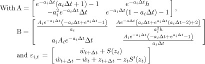
The basis of such approximations is the Taylor‐Ito expansion [Kloeden and Platen, 1995; Jimenez et al., 1999] of a SDE around a reference point x 0. Retaining only first order terms this leads to the following approximation for the SSM (1) around a reference value x 0
| (7) |
with b(x 0, Θ) = {b i(x 0, Θ)} = {Tr(ΣΣt F i,xx (x t, Θ))}, Note that for a deterministic SSM Σ = 0, we are dealing with a ODE instead of a SDE, and Eq. (7) reduces to the usual Taylor expansion. However for a SDE the Ito calculus takes into consideration a further term.
Global approximations have been mostly of the linear deterministic kind that is to say assuming Σ = 0 and taking x 0 to be fixed for the whole analysis. Unfortunately, as mentioned before, this ignores the stochastic component of the SSM. Examples with expansion around x 0 = 0 are some formulations of DCM [Friston et al., 2003; Friston et al., 2007]. This is a rather arbitrary choice and for that reason an alternative is x 0 = x s, the solution to the steady state equation f(x s,Θ) = 0. Such is the choice taken for example by [Robinson et al, 2004; Moran et al., 2007, 2008; Zetterberg et al., 1978]. As long as the system is operating around this steady state values the approximation is valid and allows transformation of the equations to the frequency domain and the analytical determination of notable properties of the system. However the linearized system does not preserve some important nonlinear properties. This is evident, for example, when several equilibrium points are present or there is a stable attractor such as a limit cycle which will not appear in the globally linearized discretization which only has a single point attractor.
For this reason many articles examine simulated trajectories of the state space variables. For the EEG most [Lopes da Silva et al., 1974; Jansen and Rit, 1995; Babajani et al., 2006] have used off the shelf methods developed for Ordinary Differential Equations (ODE). This can be problematic for several reasons. In the first place, even for deterministic SSM (where the noise component is set to zero), these methods are not guaranteed to reproduce the properties of the original continuous dynamical system, in other words they may alter the dynamical invariants of the original continuous system [Biscay et al., 1996; Carbonell et al., 2007]. For SDEs the situation is even worse. Tong has shown [Tong, 1990] that simulations of stochastic systems with polynomial based methods (such as Runge‐Kutta) are almost sure to explode. Additionally, many of these methods are computationally very expensive and are not well suited to migrate up to large scale simulations. Avoiding polynomial expansions and based on the Taylor‐Ito expansion in Eq. (7) one can obtain integration methods by retaining only the constant term which lead to the Euler (ODE) and Euler‐Maruyama (SDE) methods. These however have poor orders of convergence.
These are pitfalls avoided by the fully stochastic Local Linearization technique of Ozaki (henceforth designated the LL Method). The LL method integrates the linear approximation of the SSM (7) around the current point x 0 = x t in the orbit of the system in state space:
 |
(8) |
This integral has an exact solution which can be stated as
 |
(9) |
with  t a stochastic process with mean 0 and covariance matrix
Expression (9) is quite imposing but several different fast and accurate methods for calculating it are available. These numerical variants are known as “LL‐schemes” [Jimenez and Carbonell, 2005; De la Cruz et al., 2007] and care should be taken because some have proven to be more accurate than others. The major computational burden in these schemes is the evaluation of matrix exponentials such as e .
The LL method is accurate, stable and conserves the dynamical properties of the original continuous time system. It was first introduced by [Ozaki, 1989, 1992a], later elaborated by [Biscay et al., 1996] and extensively developed in recent years [Carbonell et al., 2002, 2005, 2006, 2007, 2008; Carbonell and Jimenez, 2008; De la Cruz et al., 2007; De la Cruz et al., 2006; Jimenez et al., 1998, 1999, 2002, 2005, 2006; Jimenez, 2002; Jimenez and Biscay, 2002; Jimenez and Carbonell, 2006]. Though originally restricted in its applications to neuroimaging [Valdes et al., 1999a, b; Riera et al., 2004, 2006, 2007], the LL method has gained popularity in recent years. A recent article incorporates it for the first time into the DCM of fMRI signals [Stephan et al., 2008] though using a less accurate LL‐scheme.
ESTIMATION OF STATE SPACE MODELS
Given data [y 1,…,y ] gathered at N t time points, in our case the EEG/fMRI measurements, it is often of interest to estimate information about the SSM under examination. The two main estimation problems are
Assuming Θ known, to estimate the x t. Predicted estimates
 are obtained sequentially from data gathered previously to time t, [y
1,…,y
t−1]. Filtered estimates
are obtained sequentially from data gathered previously to time t, [y
1,…,y
t−1]. Filtered estimates  are obtained sequentially from data gathered up to time t, [y
1,…,y
t]. Finally, smoothed estimates
are obtained sequentially from data gathered up to time t, [y
1,…,y
t]. Finally, smoothed estimates  are obtained with the whole sample of observations, [y
1,…,y
].
are obtained with the whole sample of observations, [y
1,…,y
].Assuming either filtered or smoothed estimates of the states, to estimate the parameters of the system, Θ.
The methods for estimation depend critically on the simulation (approximation) method selected. As discussed in the previous section, the type of approximation determines the properties that the estimated system will be able to exhibit. For example, with a global linear deterministic approximation of the SSM [Robinson et al., 2004; Moran et al., 2008] around a stable operating point x s, and a linear observation equation the SSM is essentially treated as a linear device. The SSM equations (including a stochastic input) how read
| (10) |
with f = f(x s,Θ), F = f x(x s,Θ), and G = g(x t,Θ,v(t)).
Transforming these equations to the frequency domain and rearranging terms yields
| (11) |
where the subscript ω indicates discrete frequencies and noise variables now have a complex multivariate Gaussian distribution. This expression can then be used to estimate the parameters Θ. In practice expression (11) is not used for parameter estimation [Robinson et al., 2004; Moran et al., 2008]. Rather the spectra (variance of complex values) of y ω are used as the data. This discards all the phase information available in the time series. It would be interesting to see if improvements in estimation could be obtained by using (11) or directly the linear SSM (10) with the methods to be described next.
Instead of global linearization, an alternative is to respect the full nonlinearities of the system by repeatedly generating EEG/fMRI simulations in the time domain (or equivalently calculating their mean and covariance at each point) and maximize their likelihood given the data by adjusting the parameters Θ. In short, we advocate the use of the the LL‐innovation method, designed to preserve the dynamical properties of the continuous time models. This method, outlined in Figure 4, was originated by T. Ozaki [1992b] and further developed in [Biscay et al., 1996; Valdes et al., 1999a, b]. It consists of the following steps:
-
1
The same LL discretization scheme described in the section on SSM simulation is used to generate a linear SDE for a given position at a trajectory in state space.
-
2
Once a locally linearized discrete state evolution is available, it can be fed together with the linearized observation equation and the data to any of several variants of the Kalman Filter in order to get predicted
 and filtered
  estimates of the states.
 -
3
Of extreme importance is that these prediction estimates may be used to estimate the innovations ϵt = y t − E[g(x , e t)] or prediction error, the extra information about a state space orbit, given the past data and after accounting for observation noise. As shown early on by Ozaki [1992b], with a properly chosen model for the dynamics, the innovations will be distributed as Gaussian white noise even if the system is highly nonlinear and the noise processes are not Gaussian.
-
4Finally in view of the Gaussian nature of the innovations, the log likelihood of the SSM given the data may be calculated as:
with Ψ(Θ)=Σ(Θ)Σ(Θ)T.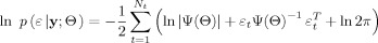
(12)
The importance of obtaining the innovations is that it removes temporal dependencies and whitens the observed time series x t into an independent series. To perform this whitening step we need to find a suitable dynamic SSM providing the prediction of the time series by using past observations. Whitening, i.e. removing the temporal dependencies on the past, and finding a suitable causal dynamic model is in fact the same thing. By whitening the causal relations are extracted from the observed time series, and a relevant dynamic model is obtained.
The concepts described so far are supported by a very strong mathematical theorem given by [Levy, 1956]; see also theorem 41 in [Protter, 1990] which states that “for any continuous‐time Markov process x(t) the corresponding innovations can be represented, under mild conditions, as the sum of two white noise processes, namely a Gaussian noise process and a Poisson noise process”. This theorem is a stronger version of the well‐known theorem for Markov diffusion processes [Ito, 1951, 1985; Doob, 1953] according to which “any dynamic process can be represented by a differential equation driven by Gaussian white noise, if the process is Markov and continuous (i.e. without any discontinuous jump)”. The case of additional observation noise has been treated by [Frost and Kailath, 1971]. Consequently we expect that, under the assumption of continuous dynamics, the time series of resulting innovations, for an optimal predictor, will be uncorrelated (in fact, independent) and Gaussian, even if, due to possible nonlinearities in dynamics, the process is non‐Gaussian distributed. This theorem implies that, if we employ a properly chosen model for the dynamics, the prediction errors will be distributed as Gaussian white noise. Then the log‐likelihood function for the time series may be calculated using the standard Gaussian likelihood, even though the original observed time series may have displayed nonlinearities and non‐Gaussian distribution.
The methodology based on Levy's theorem has been employed in time series analysis since the early 1990s [Ozaki, 1992b]. In the neurosciences it has been applied to the identification of dynamic causal models, such as the Zetterberg model for EEG time series [Valdes et al., 1999a, b] and Balloon model for fMRI time series [Riera et al., 2004]. Finally, the log‐likelihood function for the time series may be calculated using the standard Gaussian likelihood, even though the original observed time series may have displayed nonlinearities and non‐Gaussian distribution. Thus the parameter set Θ may be adjusted (using an optimization technique) to yield the maximum likelihood estimators. An evident extension is to augment the likelihood with a penalty function (negative log prior) to carry out Bayesian estimation.
The LL‐innovation approach to SSM estimation is not the only one currently available [Singer, 2008; Jimënez et al., 2006]. Popular alternatives are:
-
1
The Expectation Maximization (EM) algorithm developed by [Shumway and Stoffer, 1982]. which alternates between estimating the smoothed estimates
 and the parameters Θ.
 -
2
Monte Carlo based methods that select a set of sample points or “particles” and follow their trajectories sequentially [Chen, 2003]. Particle methods can cope with quite general SSM but are currently limited to very small scale models.
-
3
A series of methods derived from Variational Bayes techniques which reformulates the SSM by means of a path integral [Kappen, 2008; Wiegerinck and Kappen, 2006; Archambeau et al., 2007a, b]. Use of mean field approximations promise computationally very efficient estimation procedures.
-
4
A variant of these Variational techniques is the quite recent Dynamic Expectation Maximization (DEM) [Friston et al., 2007, 2008; Friston, 2008] which reformulates the SSM in terms of generalized coordinates and therefore eschews use of sequential methods such as the Kalman filter.
-
5
The Ensemble Kalman Filter (EnKF) [Evensen and van Leeuwen, 2000; Evensen, 2003] a variant of particle methods developed by geophysicists that is suited for very large scale SSM. It is to be noted that the term “ensemble” used here refers to the set of particles to be integrated using nonlinear SDE and not to “ensemble learning” which is a synonym for Variational Bayes methods.
It is to be noted that any combination of these methods may be combined with the LL integration technique to develop new estimation methods. These approaches are currently being explored. Nevertheless the LL‐innovation approach outlined here is a quite feasible alternative. Just as an example, when compared to the EM method, the latter has a higher computational cost (with a backward pass of the Kalman smoother) and yields state estimates that are not always reliable. It is also recognized that the EM algorithm may be quite slow in convergence.
SMALL SCALE EEG/fMRI MODELS
This type of modeling will illustrated with a EEG/fMRI model consisting of a single voxel housing the classical Jansen and Rit neural mass for a single cortical column [Jansen and Rit, 1995; Zetterberg et al., 1978] which is essentially the same as the Zetterberg model. This cortical module will be a component in subsequent more complicated models and is shown diagrammatically in Figure 3B. It only contains 3 interconnected populations of excitatory pyramidal (Pyr) and stellate (St) cells as well as inhibitory interneurons (Inh). Using the notation introduced for EEG/fMRI SSM, x ePSP(t) = {x (t),x (t),x (t)} for Pyr, Inh, St cells respectively. The system matrices are:
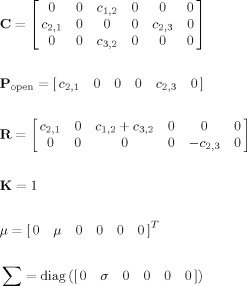 |
(13) |
Note that the only population with a stochastic input is St, assumed to be the input from the thalamus.
In this model the nPCD is generated by the transmembrane potential of Pyr. This is just the difference between EPSP and IPSP generated by St and Inh, nPCD = z (t) − z (t). For the sake of simplicity, the lead field is assumed to be K = 1, thus the EEG is equal to the nPCD. Loosely speaking this is as though we were actually measuring the Local Field Potential (LFP). The VFFS has two components u e = z 1 + z 2, the sum of EPSP and u i = z 3 the IPSP. As mentioned before, the VFSS feeds into the Metabolic Hemodynamic Model (MHM) [Sotero and Trujillo‐Barreto, 2007] (see Appendix C), a system of ordinary differential equations (ODE) depending on additional state variables x 7(t),…,x 14(t). The observed BOLD is generated by the Balloon model then is transformed to BOLD by the equation y 2(t) = g BOLD (x 13(t),x 14(t)) in Appendix C. Summarizing, for this cortical module the EEG/fMRI model the complete state vector is x(t) = {x 1(t),…,x 14(t)}. Usual values for constants in this article are listed in Appendix B. A typical simulation obtained using the LL method for integrating the SDE is shown in Figure 2C. Matlab code is provided in the supplementary material to generate this figure.
Using this type of approach, Neural Mass Modeling, has been producing for decades seemingly correct simulations of EEG rhythms (David and Friston, 2003; Lopes da Silva et al., 1974; Zetterberg et al., 1978) that not only produce EEG like signals but also predict nonlinear bifurcation behavior that can be interpreted, for example, as an explanation of epileptic seizures [Breakspear et al., 2006; Lopes da Silva et al., 2003]. In addition, as already mentioned, [Moran et al., 2007; Rowe et al., 2004] have carried out valuable theoretical analysis of EEG models [Moran et al., 2008; Robinson et al., 2004] by means of global linearization around system steady states and passing to the frequency domain. They also have fitted small scale neural mass models to EEG data by comparison of data versus model spectra.
However, to our knowledge, the first time full nonlinear neural mass models were fit to actual EEG recordings by means of the LL‐innovation method [Valdes et al., 1999a, b] used to estimate the parameters of Zetterberg's model [Zetterberg et al., 1978] for the alpha rhythm.
Fitting the parameters of this neural mass model corresponds to solving the inverse problem from the EEG to the dynamics of the ePSPs in Figure 1A. In our example, the parameters to be estimated are Θ = {c 1,2,c 2,1,c 2,3,c 3,2,μ,σ}. Unsurprisingly, the LL‐innovation approach found parameter values that, when used to produce simulated produce recordings, provided traces very similar to the original data. A new aspect was the calculation of the likelihood of the fit useful for model comparison. Even more, examination of the Gaussianity and independence of the innovations allowed the identification of several alpha rhythm recordings that could not be explained by this model‐thus providing a criterion for falsification of the theory.
What did come as a surprise was a predictive aspect of this model. The Zetterberg model exhibits a stochastic Hopf bifurcation, in which changes in parameter values transform the topology of the stable manifold in state space from a point attractor to a limit cycle. The parameters estimated for each EEG recording corresponded either to a point attractor or to a limit cycle. This model driven fingerprint for dynamic behavior was then independently confirmed with a data driven procedure. This involved fitting non parametric nonlinear time series models and ascertaining if it's “skeleton” (dynamics when the dynamic noise is turned off) was of the appropriate type. The identification of a bifurcation in a data set through model fitting is a topic of major interest. Of course, there are many types of bifurcations, each of which bear their dynamical signature in data and not all of which are displayed by a given model [Izhikevich, 2006]. Hence a complementary approach to model fitting is the visual analysis of the bifurcation structure of a given model and comparison to appropriate data as for example in [Breakspear et al., 2006]. A relevent review of combining model and data driven exploration of nonlinear dynamics can be found in [Valdés et al., 1999].
A number of biophysical models have been proposed for BOLD signals [Stephan et al., 2004]. The global approximation around a steady state and analysis in the frequency domain has also been applied to this type of model [Robinson et al., 2006].
Regarding fully nonlinear models, [Sotero and Trujillo‐Barreto, 2007] have developed a biophysical model of the coupling between neuronal activity and the BOLD signal (metabolic/hemodynamic model, MHM) that allowed explicit evaluation of the role of both excitatory and inhibitory activity. In addition to glycolysis, the “glycogen shunt” is assumed in the astrocytes. They also assume that cerebral blood flow is not directly controlled by energy usage, but it is only related to excitatory activity. Appendix C summarizes this model. By means of simulations with the LL approach, these authors successfully predicted the appearance of negative BOLD phenomena. In a subsequent article [Sotero et al., 2008], they were able to use the LL‐innovation method to fit a stochastic version of this model to BOLD signals obtained in a motor task. Using the Bayesian Information Criterion (BIC) allowed selection among several competing models. In particular it was found that observations seemed to be generated by only an excitatory population rather.
With regard to EEG/fMRI fusion, [Riera et al., 2006, 2007] were the first to use the full LL‐innovation approach for estimating a local electro vascular coupling model. LL simulations explained the continuous dynamics of electrical and vascular states within a cortical unit. They explicitly dealt with the mismatch in temporal resolution of EEG and fMRI by incorporating this information into the model. The innovation approach was then used to estimate state variables and system parameters from the EEG and BOLD signals in selected regions of interest. They applied this algorithm to recordings obtained from two subjects while passively observing a radial checkerboard with a white/black pattern reversal. The EEG and fMRI data from the first subject was used to estimate the electrical/vascular states and parameters of the model in V1.
These examples of small scale models illustrate the feasibility of creating neural mass based methods for EEG/fMRI fusion. Unfortunately it is only at this small scale that the LL‐innovation estimation has been applied. At larger scales only simulations have been possible as yet.
MEDIUM SCALE EEG/fMRI SIMULATIONS
Small scale simulations must be considered only as a proof of concept for EEG/fMRI fusion. More realistic situations must involve at least thousands of neural masses. Several issues become critical then. One problem is that of specifying the connectivities between distant neural populations since in the cortical module model the matrix C only contains local intra module connections (which we will denote as contained in the matrix C 0). [Babajani and Soltanian‐Zadeh, 2006] postulated exponential decay with distance of short range (SR) connectivity strength of both excitatory and inhibitory populations to neighboring voxels which can be included in the connectivity matrix C SR. Thus in their case they use the connectivity matrix C = C 0 + C SR. With these specifications, these authors successfully simulated EEG and the associated BOLD signals using decay parameters described in the literature. A distinctive feature of their model is the inclusion of a large number of cortical modules per voxel which addresses the issue of generator synchronization discussed on the EEG and BOLD. However, the integration methods used were standard creating the doubt if the dynamical behavior observed corresponded to the original continuous time system.
Another example of a medium sized simulation can be found in [Sotero et al., 2007]. Here the generation of EEG rhythms was studied using a model with several dozen cortical regions comprising thousands of neural masses. These regions were coupled with connectivity coefficients obtained from a neuroimaging database. This simulation included a number of new features:
Modification of the cortical module model to include Pyr to Pyr connections and 16 SDE3.
Inclusion of the thalamus as a single module as a set of 12 SDE with local connectivities which was also coupled with the cortical modules. The thalamic module consisted of an excitatory thalamic relay population receiving visual dynamic noise input. The relay population projects to cortex as well as to the inhibitory reticular thalamic population which feed back to the relay population.
Use of the connectivity matrix C = C 0 + C SR + C LR which includes in C LR the coupling strength of inter‐area or Long Range (LR) connections between large cortical areas.
Additionally, the model was modified to take into consideration conduction delays collected in the matrix T. These were used to modify the PSP functions have variable longer time courses [Jansen and Rit, 1995; Sotero et al., 2007].
A realistic lead field K was used to generate the EEG
The matrices C LR and T were defined according to their anatomical connections probability (ACP) matrix [Iturria‐Medina et al., 2007]. The ACP gives the probability that any two areas are connected at least by a single nervous fiber according to diffusion weighted Magnetic Resonance Imaging (DWMRI) techniques and Graph Theory. This matrix is estimated as follows:
-
1
The cerebral volume was represented as a non‐directed weighted graph G brain,0 = [N 0,A 0,W 0], where N 0 is the set of voxels (nodes) having a non‐zero probability of belonging to some cerebral tissue, A 0 is the set of white matter links (arcs) between contiguous voxels in N 0, and W 0 is a set of real numbers representing arcs weights. The weight of an arc is chosen so that it represents the probability that contiguous linked nodes are really connected by nervous fibers.
-
2
An iterative algorithm was employed for finding the most probable trajectory between any two nodes, which is assumed to be the hypothetical nervous fiber pathway running between these points. A node‐node anatomical connectivity measure (ranging between 0, not connected, and 1, perfectly connected) is defined as the lowest weight of the arcs set belonging to the most probable path.
-
3
After computing the node‐node connectivity measure between any two nodes of the brain surface, a threshold value of 0.6 was applied to retain values higher than 0.6, which were assigned to the matrix C LR (element cij represents the connectivity between nodes i and j).
-
4
The delay matrix T = {τi,j} i,j = 1,…,N m was estimated as the average path length between voxels (nodes), multiplied by a conduction velocity of 10 m/s. Both matrices were then averaged over neighboring voxels as to obtain the corresponding matrices for the reduced set of vertices actually used in the simulation.
The previously described model results in quite a large system of SDE. In LL schemes, the limiting step for their solution is calculating matrix exponentials. Fortunately this can now be done efficiently for sparse systems using Krylov subspace methods [Jimenez, 2002; Jimenez and Carbonell, 2005], a feature taken advantage of with the empirical sparseness of the estimated anatomical connectivity matrix as described by [Iturria‐Medina et al., 2007].
Simulations of different types of human brain rhythms were carried out in order to test the model. Changing parameter values allowed the simulation of different EEG rhythms in a similar fashion as described in [David et al., 2006a, b; David and Friston, 2003]. The simulated alpha rhythm was reactive to increase of thalamic input (visual stimulation). However alpha activity was only obtained by using in simulations the connectivity patterns estimated from DWMRI. Alpha disappeared when the elements of C LR were randomly reshuffled. This shows that the connectivity pattern assumed for EEG/fMRI simulations can be quite critical. [Sotero and Trujillo‐Barreto, 2008] then went on to augment this EEG model with their MHM model (Appendix C) for BOLD generation. The VFFS (the input to the MHM) was the number of active synapses within the voxel. The simulated EEG and BOLD signals where then subjected to the data driven EEG/BOLD correlation method described in Figure 1B. Strikingly, the observed pattern of positive BOLD‐EEG correlations in thalamus and negative BOLD‐EEG correlations in the occipital cortex present in real data (Fig. 2A) was also obtained for the simulated data (Fig. 2C).
LARGE SCALE EEG/fMRI SIMULATIONS
The previously described medium scale simulations have at most modeled a total of 1032 neural masses– the basic limitation for larger simulations is just computational. We now report a new type of integration scheme, the LL‐algebraic method, which is particularly adapted to the analysis of very large networks of neural masses. The motivation for this new type of LL scheme comes from techniques used for the analysis of electrical circuits [Schuster and Unbehauen, 2006] and other modular systems, in which the nonlinear components are described by ODE or SDE and their interconnections through algebraic equations. These types of systems which combine differential equations and algebraic equations are known as Differential Algebraic equations (DAE) and Stochastic Differential Algebraic equations (SDAE) [Denk and Winkler, 2007] and can be solved very efficiently. For example, the technique we shall use involves solving iteratively and separately the algebraic equations and the SDE [Vijalapura et al., 2005]. In fact it can easily be seen from that our neural mass models are already in a differential algebraic formulation in which Equation (3), the formula that specifies neural mass dynamics, is the differential part, and (4), the part that specifies connectivities, is the algebraic part.
The LL‐algebraic integration method alternates between two steps:
-
1
Assuming that the inputs z i(t) to each neural mass have been calculated, Eq. (3) is now a second order random differential equation (RDE). RDEs are functions of stochastic process that do not enter the equation linearly and are not necessarily Gaussian white noise (as is the case for SDE). RDEs do not pose any special problem since methods for their LL integration have been recently developed [Carbonell et al., 2005].
-
2
Given the outputs from all neural masses, the inputs z(t) may be calculated using x(t) using expression (4) z(t) = Cx(t).
Two factors may be used to speed up the simulations by orders of magnitude. One is that the numerical integration in step 1 may be carried out analytically (IV) for example using the program Mathematica 6.0 (Wolfram Research Inc.). A program for this derivation is provided in the supplementary material. Denoting the states of the i‐th neural mass states by  the integration step found analytically is:
| (14) |
 |
The second speed up factor is that, as discussed in the previous section, brain connectivity matrices are very sparse– speeding up step 2. An additional bonus of this method for integration is that the second step can now be modified to include explicitly conduction delays
| (15) |
This contrasts with the suboptimal approach of slowing down the PSP functions as has been done in [Jansen and Rit, 1995; Sotero et al., 2007].
A similar approach can be used to optimize computations for the MHM model. Careful examination of Appendix C reveals that it can be decoupled into pairs of RDE that are linked by algebraic identities. Thus these may be solved using the approach outlined above of interleaving differential and algebraic steps. The differential integration steps have also been solved analytically. Finally we mention that these integration steps for both neural masses and the MHM are all in a format that allows the use of vectorized MATLAB operations making simulation of hundreds of thousands of neural masses possible in approximately real time on a state‐of‐the‐art desktop PC. A demonstration program in MATLAB is available in the supplementary material.
In order to show the feasibility of this approach for large scale simulations, the T2 image of a normal subject was transformed to MNI space and segmented into three different brain tissues (cerebral spinal fluid, gray matter and white matter). Each individual gray matter voxel was labeled based on an anatomical atlas (constructed by manual segmentation) using the transformation matrix obtained in the previous step. All segmentation procedures were implemented by using SPM5 (Statistical Parametric Mapping, FIL, UCL) and the IBASPM (Individual Brain Atlases using SPM) toolbox (Cuban Neuroscience Center, http://www.fil.ion.ucl.ac.uk/spm/ext/#IBASPM). Then, the surfaces for the thalamus, gray and white matter (for both hemispheres) were extracted using the marching cubes algorithm as well as, the previously computed individual atlas. This yielded a set of 65,728 vertices for further analysis. This was down‐sampled to 16138 vertices for use in the simulation.
A Jansen‐Rit cortical module was placed at each of the cortical vertices (8203 for the left hemisphere, 8362 for the right hemisphere). A thalamic module was placed at each of the vertices on the thalamic surfaces (438 for the left and 465 for the right). This yielded a total of 106,614 RDEs for the neural masses to which 99,390 additional ones are added to include the MHM for each voxel. The connectivity and delay matrices were calculated as described in the section on medium scale simulations. However instead of calculating these parameters only for large cortical areas, the long range connection matrices contain all 16138 by 16138 connections and delays. Figure 5A illustrates the connections of the visual cortex. These matrices were also found empirically to be quite sparse (Fig. 5B).
Figure 5.
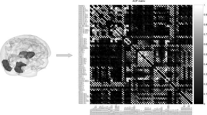
Connectivity matrix used for large scale simulations. Sample estimated nerve fiber pathways between voxels of the left and right occipital poles (left panel) of cortical tessellation shown in Figure. From these pathways anatomical connectivity values between these voxels were estimated. For use in the large scale neural mass simulations shown in Figure 2a, in reality all the voxels on both cortical and thalamic surfaces were used to calculate the overall connectivity matrix. This connectivity matrix (dimensions 16138 × 16138) is summarized for purposes of illustration here to a region to regional representation corresponding to 90 well‐known anatomical areas (right panel). The same technique also estimates the length of the fiber connections that is used to infer conduction delays between voxels. Note the extreme sparseness of connections.
Simulations were carried out based on the parameter set described in Appendix B. Resting state EEG epochs of 15.3 s duration were simulated with a Gaussian white input to the relay cells of the posterior right thalamus with mean 20 and variance 2 pulses/second. Changing levels of thalamic stimulation were achieved by increasing the input to the thalamus to a mean of 100 pulses/second during 2 s. A continuous Morlet wavelet transform was used to estimate the power in the alpha band of the Local Field Potential at each of the cortical and thalamic modules. A reference signal was calculated for each module by convolving the power at 9 Hz with a standard hemodynamic response function. The correlations between the reference signal and the simulated BOLD signal are shown in Figure 2D (left side view). It is to be noted that this simulation produces the same empirical pattern shown in Figure 2A–C.
DISCUSSION AND CONCLUSIONS
This article presents a general framework for EEG/fMRI fusion on which both data driven and model driven methods are based. For data driven methods it provides a conceptual framework for improvement. For example the framework suggests that instead of the usual approach of directly correlating hrf convolved EEG power changes with BOLD [Goldman et al., 2002; Martinez‐Montes et al., 2004], an alternative approach might be to solve the spatial inverse problem for the EEG and the temporal inverse problem for BOLD and directly compare estimates of nPCD and VFSS (Appendix A and Fig. 1C). However independently of the level of comparison, a consistent finding for all data driven analyses of EEG power in the alpha band has been that of positive correlations between EEG alpha power and BOLD in both frontal cortices and thalamus; and negative ones for the occipital region. These findings provide empirical constraints that should be a test of the predictive powers of more theoretical approaches to EEG/fMRI fusion.
We argue that the appropriate level of description for model driven fusion is the mesoscopic level that can be implemented using neural mass modeling. In this article a general model Neural Mass‐Metabolic Hemodynamic Model is set out as a State Space Model (aka DCM) that couples a neural mass EEG/fMRI model with a metabolic hemodynamic model. This model generalizes many others that have been presented before and is based upon a particularly simple form. This form consists of stating each neural mass as a distinct module and separating out the synaptic connections and conduction delays between populations as algebraic constraints, thus allowing the use of efficient numerical techniques developed for differential‐algebraic equations.
Of primary importance is to implement computer simulations that preserve the dynamical properties of the original continuous time system. We show that the Local Linearization (LL) method for integrating ordinary, stochastic, and random differential equations is appropriate for use in neural mass modeling. LL simulations of small and medium sized network were able to produce many types of EEG rhythms and were consistent with the appearance of negative BOLD signals. Additionally they reproduced the EEG/BOLD correlations found by data driven fusion methods. These simulations clearly show that the emergence of EEG rhythms depends critically on the use of realistic anatomical connectivity information estimated from DWMRI. A new LL‐algebraic method allows simulations with hundreds of thousands of neural populations and full voxel to voxel connectivities and conduction delays.
The neural mass models used in this article are derivations of the Jansen model [Jansen and Rit, 1995] and correspond to mean field approximations of integrate and fire neurons. The present framework can easily accommodate more realistic neural mass model that go beyond such simplifications by considering the second moments of neural masses [Marreiros et al., 2008] or mean field approximations of neurons with intrinsic properties [Robinson et al., 2008].
The LL integration method can be combined with many other procedures as an alternative to the Extended Kalman Filtering, the usual staple for engineering applications. In particular the LL‐innovation method for estimation consists of the discretization of the continuous time system in order to permit Kalman filtering estimate of the states as well as the data innovations or prediction errors [Galka et al., 2004; Kalman, 1960]. Under very general conditions these innovation errors will be Gaussian so the likelihood or Bayesian criteria may be easily calculated.
The LL‐innovation method has already been applied to the estimation of small scale EEG network which revealed hidden dynamical characteristics of alpha rhythm recordings that distinguish point attractor versus limit cycle behavior. This classification was then independently verified with non parametric data driven modeling. Estimation for BOLD signals allowed model selection and distinguished the contribution of inhibitory and excitatory PSPs to fMRI. Finally, combined EEG/fMRI models were able to carry out joint estimation of physiological parameters. However to avoid trivial model fitting it is important to clearly identify predictions of the EEG/fMRI model that would allow its falsification. These might be susceptible to verification via behavioral, TMS, or pharmacological modification of brain states.
EEG/fMRI should soon become a more effective tool for the explanation of inter individual differences in resting state or event related EEG. For example the increasing availability of extensive EEG/fMRI/DWMRI data sets may decide between contrasting views of the origin of brain oscillations. Such a comparison begs to be carried out between local [Lopes da Silva et al., 1974] and global [Nunez et al., 2001] models of the EEG. A perhaps more complex issue is that of EEG/fMRI fusion becoming a bridge to understand cognitive functions. For this, a junction must be made between our type of modeling and that of neural information processing systems.
Until now the LL‐innovation for estimation approach has been limited to small scale models. Fortunately there are promising developments in large scale state and parameter estimation problems, the Ensemble Kalman Filter [Evensen and van Leeuwen, 2000] and Dynamic Expectation Maximization [Friston et al., 2008] being two recent examples. Additionally, special methods are being developed for the estimation of differential algebraic systems [Becerra et al., 2001; Gerdin et al., 2007; Jorgensen et al., 2007]. It is to be expected that the combination of these techniques with the new large scale integration techniques discussed in this article will allow the estimation of realistic models with appropriate resolution in the near future. One of the most complicating factors is that even with prior DWMRI constraints the number of connectivities to be estimated may become very large. In this case the use of Bayesian estimation methods geared to finding sparse models might be necessary [Valdes‐Sosa et al., 2006].
Finally it should be emphasized that this article has limited itself to the analysis of EEG and fMRI data recorded concurrently. Many useful experiments are carried out with non concurrent data so that modifications of our model driven framework for this situation are worthwhile. A promising approach is to apply Bayesian data augmentation methods for datasets with at least partial overlap (for example to combine MEG/EEG and EEG/fMRI).
Supporting information
Additional Supporting Information may be found in the online version of this article.
Mathematica functions: There are 4 Mathematica notebooks that find the anlaytic expression for a Local Linearization (LL) step of integration of the corresponding deterministic or stochastic differntial equations. The notebooks are: cbf.nb cbvdoxy.nb glucose.nb neuralmass.nb For those that don?t have Mathematica we also append the corresponding Mathematica session in pdf form. The analytical equations are automatically translated to matlab and are the basis of the matlab demos. For more information view readme.txt included in .zip file.
Acknowledgements
The manuscript was substantially improved thanks to the thoughtful comments of 2 anonymous reviewers to whom we wish to extend our thanks. We also wish to acknowledge intensive discussions with Juan Carlos Jimenez‐Sobrino, Nelson Trujillo‐Barreto, and Lester Melie‐García. Wilmer Lobaina‐Carnet has our gratitude for the preparation of the figures.
APPENDIX A. TEMPORAL DECONVOLUTION OF THE HEMODYNAMIC RESPONSE FUNCTION
For a given voxel the following estimator for the VFFS was used:
| (A1) |
where v denotes the vector of VFFSs for time instants t = 1, …, N T, b the BOLD waveform, H the matrix form of the hemodynamic response, L the one dimensional Laplacian operator toeplitz ([−1 2–1,] T), and λ a regularizing parameter. Note that this is a temporal spline inverse solution that generalizes with a smoothness constraint the deconvolution method of Glover et al. [1999].
APPENDIX B. EXTENDED NEURAL MASS MODEL. VALUES OF PARAMETERS AND THEIR PHYSIOLOGICAL INTERPRETATION
Table .
| Parameters with the same value in all simulations | ||
|---|---|---|
| Parameter | Physiological interpretation | Value |
| A | Average synaptic gain for Excitatory, Inhibitory neurons | 3.25 mV, 22 mV |
| e 0, v 0, r | Parameters of the nonlinear sigmoid function | 5 s−1, 6 mV, 0.56 mV−1 |
| a,b,a t, b t | Average synaptic time constants for Cortex and thalamic Excitatory and Inhibitory populations. | 100 (s−1), 50, 100, 40 |
| c 1, c 3 | Synaptic contacts made by pyramidal cells on excitatory and inhibitory interneurons within a cortical module | 150, 40 |
| c 2, c 4 | Synaptic contacts made by excitatory and inhibitory interneurons on pyramidal cells within a cortical module | 120, 40 |
| c 5 | Synaptic contacts between pyramidal cells within a cortical module | 150 |
| c 6, c 7 | Synaptic contacts made by pyramidal cells on pyramidal cells of different cortical module corresponding to short and long range connections. | 50,10 |
| c 7t | Synaptic contacts made by pyramidal cells on thalamic TC cell | 100 |
| c 1t, c 3t | Synaptic contacts made by thalamic TC cells on RE and on stellate cells. | 50, 80 |
| c 2t | Synaptic contacts made by RE neurons on TC cells | 50 |
APPENDIX C. METABOLIC/HEMODYNAMIC MODEL
In Sotero and Trujillo‐Barreto (2007) the role that inhibitory and excitatory activities play in the generation of the BOLD signal was studied with the help of a biophysical model. All the variables are normalized to baseline values. According to the model, changes in excitatory (u e(t)) and inhibitory (u i(t)) neuronal activities are linked to the corresponding changes in glucose consumption, x 7(t) and x 9(t) respectively, by means of linear differential equations:
Then, the total glucose consumption is calculated as a weighted average of the excitatory and inhibitory contributions. The glucose variables were then directly related to the metabolic rates of oxygen for excitatory (m e(t)) and inhibitory (m i(t)) activities, as well as to the total oxygen consumption (m(t)):
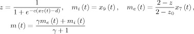 |
For describing CBF (x 11(t)) dynamics, the MHM uses the model introduced in Friston et al. (2000) but with the additional assumption that CBF is not coupled to inhibitory activity:
As in earlier approaches, in the MHM (Sotero and Trujillo‐Barreto, 2007) the Balloon model (Buxton et al, 2004) is employed for linking the output of the metabolic and vascular models to normalized cerebral blood volume (x 13(t)) and deoxyhemoglobin content (x 14(t)).
Knowing x 13(t) and x 14(t), the BOLD signal is calculated as in Buxton et al. (2004):
The interpretation and values of MHM parameters are displayed in the following table:
Table .
| Parameter | Interpretation | Value | |
|---|---|---|---|
| a e | Efficacy of glucose consumption response to excitation | 1 | |
| a i | Efficacy of glucose consumption response to inhibition | 1 | |
| τe | Time‐constant of the excitatory glucose consumption impulse response. | 1 | |
| τi | Time‐constant of the inhibitory glucose consumption impulse response | 0.8 | |
| c | Steepness of the sigmoid function x | 2.5 | |
| d | Position of the threshold of the sigmoid function x | 1.6 | |
| δe | Delay between excitatory neuronal activity and corresponding glucose consumption. | 0.1 s | |
| δi | Delay between inhibitory neuronal activity and corresponding glucose consumption. | 0.1 s | |
| δf | Delay between excitatory neuronal activity and CBF response | 0.2 s | |
| γ | Baseline ratio of excitatory to inhibitory synaptic activity in the voxel | 5 | |
| ε | Efficacy of blood flow response to excitation | 0.6 | |
| τs | Constant for CBF signal decay | 1.5 (Friston et al., 2000) | |
| τf | Constant for CBF autoregulatory feedback | 2.4 (Friston et al., 2000) | |
| τ0 | Transit time through the balloon | 1 s (Buxton et al., 2004) | |
| α | Coefficient of the steady state flow‐volume relationship | 0.4 (Buxton et al., 2004) | |
| a1 | Weight for deoxyhemoglobin change | 3.4 (Buxton et al., 2004) | |
| a2 | Weight for blood volume change | 1 (Buxton et al., 2004) | |
|
|
Baseline blood volume | 0.02 (Friston et al., 2000) |
APPENDIX D. EXPLICIT EQUATIONS FOR LL INTEGRATION OF A NEURAL MASS
As described in (Carbonell et al., 2005) the local linearization of a Random Differential (RDE) is as follows. Let's assume that a k‐dimensional random process q(t), t∈ [t 0,T] and a nonlinear function f are given and define the d‐dimensional RDE
Then, given a step size Δt, the local linearization scheme that solves numerically the equation above at the time instants t n = t 0 + nΔt, n = 0,1,…. is given by:
where L = [I d, 0dx2], r = [01x(d+1),1]T and the (d + 2) × (d + 2) matrix C n is defined by blocks as
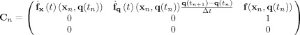 |
(A2) |
Now consider the neural mass:
| (A3) |
The required Jacobian matrices are
| (A4) |
Substituting expressions (A3) and (A4) into the formula (A2) produces an expression which can be solved symbolically making it possible to obtain expression (14) in the main text. A Mathematca 6.0 (Wolfram Research Inc.) program to do this is included in the supplementary material. A similar analysis is valid for the MHM equations (Appendix C). Note that these equations for the MHM are organized in pairs with algebraic constraints linking them. Thus it is possible to use the same strategy as just outlined for the neural mass.
Footnotes
Mathematical Notation: lower case Latin symbols f denote scalars, lower case bold symbols f vectors, upper case symbols F matrices, and Greek letters ϕ unknown parameters. F
T is the transpose of F, Tr(F) its trace, F
−1 its inverse,  its determinant.
  the derivative of the time dependent function f(t) F
x(x
0) is the Jacobian matrix of derivatives of with f respect to x, evaluated at x = x
0,
the derivative of the time dependent function f(t) F
x(x
0) is the Jacobian matrix of derivatives of with f respect to x, evaluated at x = x
0,  . Similarly, the Hessian matrix of f with respect to its i‐th component is defined as
 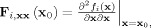 . f
t shall denote the value at time instant t of the discretized process f(t). diag (f) will denote the diagonal matrix with elements of f on the main diagonal. The matrix toeplitz(f) will denote the symmetric matrix with each elements of f along the corresponding diagonal.
. f
t shall denote the value at time instant t of the discretized process f(t). diag (f) will denote the diagonal matrix with elements of f on the main diagonal. The matrix toeplitz(f) will denote the symmetric matrix with each elements of f along the corresponding diagonal.
According to stochastic differential calculus (Protter, 1990; Ito, 1951, 1985) the derivative  does not actually exist since w(t) is a Wiener process or Brownian motion that is nowhere differentiable. In that formalism the equations for a SDE are actually expressed in terms of differentials which are a shorthand to denote stochastic integral.
In reality Random Differential Equations, but see (Carbonell et al., 2007) for the equivalence in this particular case.
REFERENCES
- Archambeau C,Opper M,Shen Y,Cornford D,Shawe‐Taylor J ( 2007a): Variational inference for diffusion processes In Platt C.,Koller D.,Singer Y.,Roweis S. editors, Neural Information Processing Systems (NIPS) 20, 2008. The MIT Press; Cambridge. Massachusetts: pp. 17–24. [Google Scholar]
- Archambeau C,Cornford D,Opper M,Shawne‐Talyor J. ( 2007b): Gaussian process approximations of stochastic differential equations. JMLR: Workshop and Conference Proceedings. pp. 1–16. [Google Scholar]
- Attwell DF,Iadecola C ( 2002): The neural basis of functional brain imaging signals. Trends Neurosci 25: 621–625. [DOI] [PubMed] [Google Scholar]
- Babajani A,Soltanian‐Zadeh H ( 2006): Integrated MEG/EEG and fMRI model based on neural masses. IEEE Trans Biomed Eng 53: 1794–1801. [DOI] [PubMed] [Google Scholar]
- Babajani A,Nekooei MH,Soltanian‐Zadeh H ( 2005): Integrated MEG and fMRI model: Synthesis and analysis. Brain Topogr 18: 101–113. [DOI] [PubMed] [Google Scholar]
- Becerra VM,Roberts PD,Griffiths GW ( 2001): Applying the extended Kalman filter to systems described by nonlinear differential‐algebraic equations. Control Eng Pract 9: 267–281. [Google Scholar]
- Biscay R,Jimenez JC,Riera JJ,Valdes PA ( 1996): Local linearization method for the numerical solution of stochastic differential equations. Ann Inst Stat Math 48: 631–644. [Google Scholar]
- Bosch‐Bayard J,Valdes‐Sosa P,Virues‐Alba T,Aubert‐Vazquez E,John ER,Harmony T ( 2001): 3D statistical parametric mapping of EEG source spectra by means of Variable Resolution Electromagnetic Tomography (VARETA). Clin Electroencephalogr 32: 47–61. [DOI] [PubMed] [Google Scholar]
- Breakspear M,Roberts JA,Terry JR,Rodrigues S,Mahant N,Robinson PA ( 2006): A unifying explanation of primary generalized seizures through nonlinear brain modeling and bifurcation analysis. Cereb Cortex 16: 1296–1313. [DOI] [PubMed] [Google Scholar]
- Buxton RB,Uludag K,Dubowitz DJ,Liu TT ( 2004): Modeling the hemodynamic response to brain activation. NeuroImage 23: S220–S223. [DOI] [PubMed] [Google Scholar]
- Buzsaki G,Draguhn A ( 2004): Neuronal oscillations in cortical networks. Science 304: 1926–1929. [DOI] [PubMed] [Google Scholar]
- Carbonell F,Jimenez JC ( 2008): Weak local linear discretizations for stochastic differential equations with jumps. J Appl Probability 45: 201–210. [Google Scholar]
- Carbonell F,Jimenez JC,Biscay R ( 2002): A numerical method for the computation of the Lyapunov exponents of nonlinear ordinary differential equations. Appl Math Comput 131: 21–37. [Google Scholar]
- Carbonell F,Jimenez JC,Biscay RJ,De la Cruz H ( 2005): The local linearization method for numerical integration of random differential equations. Bit Numeric Math 45: 1–14. [Google Scholar]
- Carbonell F,Jimenez JC,Biscay RJ ( 2006): Weak local linear discretizations for stochastic differential equations: Convergence and numerical schemes. J Comput Appl Math 197: 578–596. [Google Scholar]
- Carbonell F,Biscay R,Jimenez JC,De la Cruz H ( 2007): Numerical simulation of nonlinear dynamical systems driven by commutative noise. J Comput Phys 226: 1219–1233. [Google Scholar]
- Carbonell F,Jimenez JC,Pedroso LM ( 2008): Computing multiple integrals involving matrix exponentials. J Comput Appl Math 213: 300–305. [Google Scholar]
- Chen Z ( 2003):Bayesian Filtering: From Kalman Filters to Particle Filters, and Beyond . http://users.isr.ist.utl.pt/~jpg/tfc0607/chen_bayesian.pdf
- Chen CC,Kiebel SJ,Friston KJ ( 2008): Dynamic causal modelling of induced responses. Neuroimage 41: 1293–1312. [DOI] [PubMed] [Google Scholar]
- Coombes S,Venkov NA,Shiau L,Bojak I,Liley DTJ,Laing CR ( 2007): Modeling electrocortical activity through improved local approximations of integral neural field equations. Phys Rev E 76: 051901–051908. [DOI] [PubMed] [Google Scholar]
- Daunizeau J,Grova C,Marrelec G,Mattout J,Jbabdi S,Pelegrini‐Issac M ( 2007): Symmetrical event‐related EEG/fMRI information fusion in a variational Bayesian framework. Neuroimage 36: 69–87. [DOI] [PubMed] [Google Scholar]
- David O,Friston KJ ( 2003): A neural mass model for MEG/EEG: Coupling and neuronal dynamics. Neuroimage 20: 1743–1755. [DOI] [PubMed] [Google Scholar]
- David O,Friston KJ,Harrison LM ( 2006a): Neuronal models of EEEG and MEG In: Friston KJ,editor. Statistical Parametric Mapping: The Analysis of Functional Brain Images, 1st ed UK: Academic Press; pp 414–440. [Google Scholar]
- David O,Kiebel SJ,Harrison LM,Mattout J,Kilner JM,Friston KJ ( 2006b): Dynamic causal modeling of evoked responses in EEG and MEG. Neuroimage 30: 1255–1272. [DOI] [PubMed] [Google Scholar]
- David O,Kilner JM,Friston KJ ( 2006c): Mechanisms of evoked and induced responses in MEG/EEG. Neuroimage 31: 1580–1591. [DOI] [PubMed] [Google Scholar]
- De la Cruz H,Biscay RJ,Carbonell F,Jimenez JC,Ozaki T ( 2006): Local Linearization‐Runge Kutta (LLRK) methods for solving ordinary differential equations Computational Science – Iccs 2006,Part 1, Proceedings, 3991, Heidelberg: Springer Berlin; pp 132–139. [Google Scholar]
- De la Cruz H,Biscay RJ,Carbonell F,Ozaki T,Jimenez JC ( 2007): A higher order local linearization method for solving ordinary differential equations. Appl Math Comput 185: 197–212. [Google Scholar]
- Denk G,Winkler R ( 2007): Modelling and simulation of transient noise in circuit simulation. Math Comput Model Dyn Syst 13: 383–394. [Google Scholar]
- Doob JL ( 1953): Stochastic Processes. New York: Wiley. [Google Scholar]
- Engel AK,Fries P,Singer W ( 2001): Dynamic predictions: Oscillations and synchrony in top‐down processing. Nat Rev Neurosci 2: 704–716. [DOI] [PubMed] [Google Scholar]
- Evensen G ( 2003): The Ensemble Kalman Filter: Theoretical formulation and practical implementation. Ocean Dyn 53: 343–367. [Google Scholar]
- Evensen G,van Leeuwen PJ ( 2000): An ensemble Kalman smoother for nonlinear dynamics. Monthly Weather Rev 128: 1852–1867. [Google Scholar]
- Fox MD,Raichle ME ( 2007): Spontaneous fluctuations in brain activity observed with functional magnetic resonance imaging. Nat Rev Neurosci 8: 700–711. [DOI] [PubMed] [Google Scholar]
- Friston KJ ( 1994): Functional and effective connectivity in neuroimaging: A synthesis. Hum Brain Mapp 2: 56–78. [Google Scholar]
- Friston K ( 2006): Dynamic causal modelling of brain responses. J Psychophysiol 20: 322. [Google Scholar]
- Friston KJ ( 2008): Variational filtering. Neuroimage 41: 747–766. [DOI] [PubMed] [Google Scholar]
- Friston KJ,Harrison L,Penny W ( 2003): Dynamic causal modelling. Neuroimage 19: 1273–1302. [DOI] [PubMed] [Google Scholar]
- Friston K,Mattout J,Trujillo‐Barreto N,Ashburner J,Penny W ( 2007): Variational free energy and the Laplace approximation. Neuroimage 34: 220–234. [DOI] [PubMed] [Google Scholar]
- Friston KJ,Trujillo‐Barreto N,Daunizeau J ( 2008): DEM: A variational treatment of dynamic systems. Neuroimage 41: 849–885. [DOI] [PubMed] [Google Scholar]
- Frost PA,Kailath T ( 1971): An innovation approach to least squares estimation. III. Nonlinear estimation in white Gaussian noise. IEEE Trans Autom Contr 16: 217–226. [Google Scholar]
- Galka A,Yamashita O,Ozaki T,Biscay R,Valdes‐Sosa P ( 2004): A solution to the dynamical inverse problem of EEG generation using spatiotemporal Kalman filtering. Neuroimage 23: 435–453. [DOI] [PubMed] [Google Scholar]
- Gerdin M,Schon TB,Glad T,Gustafsson F,Ljung L ( 2007): On parameter and state estimation for linear differential‐algebraic equations. Automatica 43: 416–425. [Google Scholar]
- Glover GH ( 1999): Deconvolution of impulse response in event‐related BOLD fMRI. Neuroimage 9: 416–429. [DOI] [PubMed] [Google Scholar]
- Goldman RI,Stern JM,Engel J,Cohen MS ( 2002): Simultaneous EEG and fMRI of the alpha rhythm. Neuroreport 13: 2487–2492. [DOI] [PMC free article] [PubMed] [Google Scholar]
- Harrison LM,David O,Friston KJ ( 2006): Neuronal models of ensemble dynamics In: Friston KJ,editor. Statistical Parametric Mapping: The Analysis of Functional Brain Images,1st ed UK: Academic Press; pp 391–405. [Google Scholar]
- Ito K ( 1951): On stochastic differential equations. Mem Am Math Soc 4: 1–51. [Google Scholar]
- Ito K ( 1985): An outline of development of the theory of stochastic‐processes. Stochastic Process Appl 21: 5. [Google Scholar]
- Iturria‐Medina Y,Canales‐Rodriguez EJ,Melie‐Garcia L,Valdes‐Hernandez PA,Martinez‐Montes E,Aleman‐Gomez Y, et al. ( 2007): Characterizing brain anatomical connections using diffusion weighted MRI and graph theory. Neuroimage 36: 645–660. [DOI] [PubMed] [Google Scholar]
- Ives JR,Warach S,Schmitt F,Edelman RR,Schomer DL ( 1993): Monitoring the patients EEG during Echo‐Planar Mri. Electroencephalogr Clin Neurophysiol 87: 417–420. [DOI] [PubMed] [Google Scholar]
- Izhikevich EM ( 2006): Dynamical Sytems in Neuroscience: The Geometry of Excitability and Bursting. Cambridge, MA: MIT Press. [Google Scholar]
- Izhikevich EM,Edelman GM ( 2008): Large‐scale model of mammalian thalamocortical systems. Proc Natl Acad Sci USA 105: 3593–3598. [DOI] [PMC free article] [PubMed] [Google Scholar]
- Jansen BH,Rit VG ( 1995): Electroencephalogram and visual‐evoked potential generation in a mathematical‐model of coupled cortical columns. Biol Cyber 73: 357–366. [DOI] [PubMed] [Google Scholar]
- Jimenez JC ( 2002): A simple algebraic expression to evaluate the local linearization schemes for stochastic differential equations. Appl Math Lett 15: 775–780. [Google Scholar]
- Jimenez JC,Biscay RJ ( 2002): Approximation of continuous time stochastic processes by the local linearization method revisited. Stochastic Anal Appl 20: 105–121. [Google Scholar]
- Jimënez JC,Biscay R,Ozaki T ( 2006): Inference methods for discretely observed continuous‐time stochastic volatility models: A commented overview. Asian‐Pacific Financial Markets 12: 109–141. [Google Scholar]
- Jimenez JC,Valdes PA,Rodriguez LM,Riera JJ,Biscay R ( 1998): Computing the noise covariance matrix of the local linearization scheme for the numerical solution of stochastic differential equations. Appl Math Lett 11: 19–23. [Google Scholar]
- Jimenez JC,Shoji I,Ozaki T ( 1999): Simulation of stochastic differential equations through the local linearization method. A comparative study. J Stat Phys 94: 587–602. [Google Scholar]
- Jimenez JC,Carbonell F ( 2005): Rate of convergence of local linearization schemes for initial‐value problems. Appl Math Comput 171: 1282–1295. [Google Scholar]
- Jimenez JC,Carbonell F ( 2006): Local linear approximations of jump diffusion processes. J Appl Probability 43: 185–194. [Google Scholar]
- Jimenez JC,Biscay R,Mora C,Rodriguez LM ( 2002): Dynamic properties of the local linearization method for initial‐value problems. Appl Math Comput 126: 63–81. [Google Scholar]
- Jimenez JC,Pedroso LM,Carbonell F,Hernandez V ( 2006): Local linearization method for numerical integration of delay differential equations. SIAM J Numer Anal 44: 2584–2609. [Google Scholar]
- Jorgensen JB,Kristensen MR,Thomsen PG,Madsen H ( 2007): New extended Kalman filter algorithms for Stochastic differential algebraic equations. Assess Future Directions Nonlinear Model Predictive Control 358: 359–366. [Google Scholar]
- Kalman RE ( 1960): A new approach to linear filtering and predicition problems. Trans ASME J Basic Eng 82: 35–45. [Google Scholar]
- Kappen HJ ( 2008): An introduction to stochastic control theory, path integrals and reinforcement learning . http://www.snn.ru.nl/~bertk/kappen_granada2006.pdf.
- Kloeden PE,Platen E ( 1995): Numerical Solutin of Stochastic Differential Equations, 2nd Corrected Printing ed Berlin‐ Heidelberg‐New York: Springer Verlga. [Google Scholar]
- Laufs H ( 2008): Endogenous brain oscillations and related networks detected by surface EEG‐combined fMRI. Hum Brain Mapp 29: 762–769. [DOI] [PMC free article] [PubMed] [Google Scholar]
- Laufs H,Kleinschmidt A,Beyerle A,Eger E,Salek‐Haddadi A,Preibisch C ( 2003): EEG‐correlated fMRI of human alpha activity. Neuroimage 19: 1463–1476. [DOI] [PubMed] [Google Scholar]
- Laufs H,Daunizeau J,Carmichael DW,Kleinschmidt A ( 2008): Recent advances in recording electrophysiological data simultaneously with magnetic resonance imaging. Neuroimage 40: 515–528. [DOI] [PubMed] [Google Scholar]
- Levy P ( 1956): Sur une classe de courbes de l'espace de Hilbert et sur une equation integrale non lineaire. Ann Sci Ecole Norm Sup 73: 121–156. [Google Scholar]
- Liu AK,Belliveau JW,Dale AM ( 1998): Spatiotemporal imaging of human brain activity using functional MRI constrained magnetoencephalography data: Monte Carlo simulations. Proc Natl Acad Sci USA 95: 8945–8950. [DOI] [PMC free article] [PubMed] [Google Scholar]
- Logothetis NK ( 2002): The neural basis of the blood‐oxygen‐level‐dependent functional magnetic resonance imaging signal. Philos Trans Roy Soc London Ser B 357: 1003–1037. [DOI] [PMC free article] [PubMed] [Google Scholar]
- Lopes da Silva FH,Blanes W,Kalitzin SN,Parra J,Suffczynski P,Velis DN ( 2003): Epilepsies as dynamical diseases of brain systems: Basic models of the transition between normal and epileptic activity. Epilepsia 44: 72–83. [DOI] [PubMed] [Google Scholar]
- Lopes da Silva FH,Hoeks A,Smits H,Zetterbe LH ( 1974): Model of brain rhythmic activity—Alpha‐rhythm of thalamus. Kybernetik 15: 27–37. [DOI] [PubMed] [Google Scholar]
- Mantini D,Perrucci MG,Del Gratta C,Romani GL,Corbetta M ( 2007): Electrophysiological signatures of resting state networks in the human brain. Proc Natl Acad Sci USA 104: 13170–13175. [DOI] [PMC free article] [PubMed] [Google Scholar]
- Marreiros AC,Daunizeau J,Kiebel SJ,Friston KJ ( 2008): Population dynamics: Variance and the sigmoid activation function. Neuroimage 42: 147–157. [DOI] [PubMed] [Google Scholar]
- Martinez‐Montes E,Valdes‐Sosa PA,Miwakeichi F,Goldman RI,Cohen MS ( 2004): Concurrent EEG/fMRI analysis by multiway Partial Least Squares. Neuroimage 22: 1023–1034. [DOI] [PubMed] [Google Scholar]
- Miwakeichi F,Martinez‐Montes E,Valdes‐Sosa PA,Nishiyama N,Mizuhara H,Yamaguchi Y ( 2004): Decomposing EEG data into space‐time‐frequency components using Parallel Factor Analysis. Neuroimage 22: 1035–1045. [DOI] [PubMed] [Google Scholar]
- Moran RJ,Kiebel SJ,Stephan KE,Reilly RB,Daunizeau FKJ ( 2007). A neural mass model of spectral responses in electrophysiology. Neuroimage 37: 706–720. [DOI] [PMC free article] [PubMed] [Google Scholar]
- Moran RJ,Stephan KE,Kiebel SJ,Rombach N,O'Connor WT,Murphy KJ ( 2008): Bayesian estimation of synaptic physiology from the spectral responses of neural masses. NeuroImage 42: 272–284. [DOI] [PMC free article] [PubMed] [Google Scholar]
- Nunez PL,Silberstein RB ( 2000): On the relationship of synaptic activity to macroscopic measurements: Does co‐registration of EEG with fMRI make sense? Brain Topography 13: 79–96. [DOI] [PubMed] [Google Scholar]
- Nunez PL,Wingeier BM,Silberstein RB ( 2001): Spatial‐temporal structures of human alpha rhythms: Theory, microcurrent sources, multiscale measurements, and global binding of local networks. Hum Brain Mapp 13: 125–164. [DOI] [PMC free article] [PubMed] [Google Scholar]
- Ozaki T ( 1989): Statistical identification of nonlinear random vibration systems. J Appl Mech–Trans ASME 56: 186–191. [Google Scholar]
- Ozaki T ( 1992a) A bridge between nonlinear time‐series models and nonlinear stochastic dynamic‐systems—A local linearization approach. Statistica Sinica 2: 113–135. [Google Scholar]
- Ozaki T ( 1992b): Identification of nonlinearities and non‐Gaussianities in time series In: Brillinger D,Caines P, Geweke J,Parzen E,Rosenblatt M, Taqqu M, editors.New Directions in Time Series Analysis, Part I, IMA Volumes in Mathematics and Its Application, Vol. 45, Berlin: Springer; pp. 227–264. [Google Scholar]
- Protter P ( 1990): Stochastic Integration and Differential Equations. Berlin: Springer. [Google Scholar]
- Riera JJ,Watanabe J,Kazuki T,Naoki M,Aubert E,Ozaki T, et al. ( 2004): A state‐space model of the hemodynamic approach: Nonlinear filtering of BOLD signals. Neuroimage 21: 547–567. [DOI] [PubMed] [Google Scholar]
- Riera JJ,Wan XH,Jimenez JC,Kawashima R ( 2006): Nonlinear local electrovascular coupling. I. A theoretical model. Hum Brain Mapp 27: 896–914. [DOI] [PMC free article] [PubMed] [Google Scholar]
- Riera JJ,Jimenez JC,Wan X,Kawashima R,Ozaki T ( 2007): Nonlinear local electrovascular coupling. II. From data to neuronal masses. Hum Brain Mapp 28: 335–354. [DOI] [PMC free article] [PubMed] [Google Scholar]
- Riera JJ,Schousboe A,Waagepetersen S,Howarth C,Hyder F ( 2008): The micro‐architecture of the cerebral cortex: Functional neuroimaging models and metabolism. NeuroImage 40: 1436–1459. [DOI] [PMC free article] [PubMed] [Google Scholar]
- Ritter P,Villringer A ( 2006): Simultaneous EEG‐fMRI. Neurosci Biobehav Rev 30: 823–838. [DOI] [PubMed] [Google Scholar]
- Robinson PA,Rennie CJ,Rowe DL,O'Connor SC ( 2004): Estimation of multiscale neurophysiologic parameters by electroencephalographic means. Hum Brain Mapp 23: 53–72. [DOI] [PMC free article] [PubMed] [Google Scholar]
- Robinson PA,Drysdale PM,Van der MH,Kyriakou E,Rigozzi MK,Germanoska B ( 2006): BOLD responses to stimuli: Dependence on frequency, stimulus form, amplitude, and repetition rate. Neuroimage 31: 585–599. [DOI] [PubMed] [Google Scholar]
- Robinson PA,Wu H,Kim JW ( 2008): Neural rate equations for bursting dynamics derived from conductance‐based equations. J Theoretical Biol 250: 663–672. [DOI] [PubMed] [Google Scholar]
- Rowe DL,Robinson PA,Rennie CJ ( 2004): Estimation of neurophysiological parameters from the waking EEG using a biophysical model of brain dynamics. J Theoretical Biol 231: 413–433. [DOI] [PubMed] [Google Scholar]
- Schuster M,Unbehauen R ( 2006): Analysis of nonlinear electric networks by means of differential algebraic equations solvers. Electrical Eng 88: 229–239. [Google Scholar]
- Shumway RH,Stoffer DS ( 1982): An Approach to time series smoothing and forecasting using the em algorithm. J Time Series Anal 3: 253–264. [Google Scholar]
- Singer H ( 2008): Nonlinear continuous time modeling approaches in panel research. Statistica Neerlandica 62: 29–57. [Google Scholar]
- Sotero RC,Trujillo‐Barreto NJ ( 2007): Modelling the role of excitatory and inhibitory neuronal activity in the generation of the BOLD signal. Neuroimage 35: 149–165. [DOI] [PubMed] [Google Scholar]
- Sotero RC,Trujillo‐Barreto NJ ( 2008): Biophysical model for integrating neuronal activity, EEG, fMRI and metabolism. Neuroimage 39: 290–309. [DOI] [PubMed] [Google Scholar]
- Sotero RC,Trujillo‐Barreto NJ,Iturria‐Medina Y,Carbonell F,Jimenez JC ( 2007): Realistically coupled neural mass models can generate EEG rhythms. Neural Comput 19: 478–512. [DOI] [PubMed] [Google Scholar]
- Sotero RC,Trujillo‐Barreto NJ,Jiménez JC,Carbonell F,Rodríguez‐Rojas R ( 2008): Identification and comparison of stochastic metabolic/hemodynamics model (sMHM) for the generation of the BOLD signal. J Comput Neurosci DOI 10.1007 / s10827‐008‐0109‐3. [DOI] [PubMed] [Google Scholar]
- Stephan KE,Harrison LM,Penny WD,Friston KJ ( 2004): Biophysical models of fMRI responses. Curr Opin Neurobiol 14: 629–635. [DOI] [PubMed] [Google Scholar]
- Stephan KE,Kapser L,Harrison LM,Daunizeau J,van Ouden HEM,Breakspear M ( 2008): Nonlinear dynamic causal models for fMRI. Neuroimage 42: 649–662. [DOI] [PMC free article] [PubMed] [Google Scholar]
- Tong H ( 1990). Nonlinear Time Series: A Dynamical System Approach. Oxford: Clarendon Press. [Google Scholar]
- Trujillo‐Barreto NJ,Martínez‐Montes E,Melie‐García L,Valdés‐Sosa PA ( 2001): A symmetrical Bayesian Model for fMRI and EEG/MEG Neuroimage Fusion. IJBEM 3. [Google Scholar]
- Trujillo‐Barreto NJ,Aubert‐Vazquez E,Valdes‐Sosa PA ( 2004): Bayesian model averaging in EEG/MEG imaging. Neuroimage 21: 1300–1319. [DOI] [PubMed] [Google Scholar]
- Valdés P,Bosch J,Jiménez JC,Trujillo N,Biscay LR,Morales F ( 1999a): The statistical identification of nonlinear brain dynamics: A progress report In: Pradlan N, Rapp PE, Sreenivasan R, editors, Nonlinear Dynamics and Brain functioning, New York: Nova Science; pp 243–264. [Google Scholar]
- Valdes PA,Jimenez JC,Riera J,Biscay R,Ozaki T ( 1999b): Nonlinear EEG analysis based on a neural mass model. Biol Cybernet 81: 415–424. [DOI] [PubMed] [Google Scholar]
- Valdes‐Sosa PA,Bornot JM,Vega M,Melie L,Lage A,Canales E ( 2006): Granger causality on spatial manifolds: Applications to neuroimaging In: Schelter B,Winterhalder M, Timmer J, editors. Handbook of Time Series Analysis. Berlin: Wiley‐VCH; pp 461–485. [Google Scholar]
- Varela F,Lachaux JP,Rodriguez E,Martinerie J ( 2001): The brainweb: Phase synchronization and large‐scale integration. Nat Rev Neurosci 2: 229–239. [DOI] [PubMed] [Google Scholar]
- Vijalapura PK,Strain J,Govindjee S ( 2005): Fractional step methods for index‐1 differential‐algebraic equations. J Comput Phys 203: 305–320. [Google Scholar]
- Wiegerinck W,Kappen B ( 2006): A Gaussian approximation for stochastic nonlinear dynamical processes with annihilation. In NIPS 2006 Workshop on Dynamical Systems, Stochastic Processes and Bayesian Inference. Whistler, BC, Canada..
- Wilson HR,Cowan JD ( 1972): Excitatory and inhibitory interactions in localized populations of model neurons. Biophys J 12, 1–24. [DOI] [PMC free article] [PubMed] [Google Scholar]
- Zetterberg LH,Kristiansson L,Mossberg K ( 1978): Performance of a model for a local neuron population. Biol Cybernet 31: 15–26. [DOI] [PubMed] [Google Scholar]
Associated Data
This section collects any data citations, data availability statements, or supplementary materials included in this article.
Supplementary Materials
Additional Supporting Information may be found in the online version of this article.
Mathematica functions: There are 4 Mathematica notebooks that find the anlaytic expression for a Local Linearization (LL) step of integration of the corresponding deterministic or stochastic differntial equations. The notebooks are: cbf.nb cbvdoxy.nb glucose.nb neuralmass.nb For those that don?t have Mathematica we also append the corresponding Mathematica session in pdf form. The analytical equations are automatically translated to matlab and are the basis of the matlab demos. For more information view readme.txt included in .zip file.