An fMRI normative database for connectivity networks using one‐class support vector machines

Abstract

The application of functional magnetic resonance imaging (fMRI) in neuroscience studies has increased enormously in the last decade. Although primarily used to map brain regions activated by specific stimuli, many studies have shown that fMRI can also be useful in identifying interactions between brain regions (functional and effective connectivity). Despite the widespread use of fMRI as a research tool, clinical applications of brain connectivity as studied by fMRI are not well established. One possible explanation is the lack of normal patterns and intersubject variability—two variables that are still largely uncharacterized in most patient populations of interest. In the current study, we combine the identification of functional connectivity networks extracted by using Spearman partial correlation with the use of a one‐class support vector machine in order construct a normative database. An application of this approach is illustrated using an fMRI dataset of 43 healthy subjects performing a visual working memory task. In addition, the relationships between the results obtained and behavioral data are explored. Hum Brain Mapp, 2009. © 2008 Wiley‐Liss, Inc.

INTRODUCTION

Neuroimaging has played a fundamental role in the study of human behavior and neuroscience. Functional magnetic resonance imaging (fMRI), based on the blood oxygenation level dependent (BOLD) signal, is one of the most commonly used tools in this field and has been the basis of many studies of cognitive processing in brain mapping research. Since its first description by Ogawa et al. [ 1990], the number of studies involving BOLD fMRI has increased rapidly [Bandettini, 2007], emphasizing the current importance of this technique.

The majority of fMRI literature is confined to the description of brain regions that are activated by certain stimuli. However, the network‐level nature of much brain activity requires, in addition, the quantification and understanding of interactions between brain regions, i.e., connectivity analysis. Structural equation (SEM, McIntosh [ 1999]) and dynamic causal models (DCM, Friston et al. [ 2003]) have been the most commonly used approaches to investigate connectivity in fMRI. However, in original forms, these approaches require the prior specification of a model describing inter‐regional connections. Marrelec et al. [ 2006, 2007] suggested the application of partial correlation analysis (PCrA) which does not require prespecification of connectivity structure or models. PCrA measures the dependence between two random variables whilst controlling for the influences of a set of other variables and as such, is useful for identifying direct relationships. The main limitation of PCrA is that it only quantifies dependencies and does not describe the influences between brain areas, i.e., there is no inference of causality or directionality. However, PCrA is a simple and reliable technique to describe functionally connected networks and it is possible to infer causality qualitatively by other information available in literature (e.g., studies in rats or primates).

Pattern recognition methods such as Support Vector Machines (SVMs) have been widely used to analyze fMRI data [Mitchell et al., 2004; Mourao‐Miranda et al., 2005, 2006, 2007; Wang et al., 2003, 2007]. In these applications, fMRI volumes are treated as spatial samples and SVMs are used to identify statistical properties of the data that discriminate between groups of subjects or brain states. An extension of “classical” SVM is the one‐class support vector machine [OC‐SVM Campbell and Bennett, 2001; Schölkopf et al., 2001; Tax and Duin, 1999]. OC‐SVM has been applied with success in Bioinformatics, to identify compounds, which inhibit CYP3A4 [Kriegl et al., 2005] to detect horizontal gene transfer in several genomes [Tsirigos and Rigoutsos, 2005] and to predict protein–protein interaction [Alashwal et al., 2006]. Zhou et al. [ 2005] proposed the application of OC‐SVM for the identification of brain tumors using structural MRI images. Song et al. [ 2007] introduced OC‐SVM to detect “novelty” or outlying behavior in brain activity measured using fMRI. Basically, OC‐SVM has the ability to estimate population quantiles from a set of multidimensional samples in a nonparametric fashion. After training OC‐SVM using a set of examples, one may assess whether a new observation is likely to belong to the training data population, with a controlled probability of misclassification. OC‐SVM is an attractive approach in medical research because given a set of variables measured in normal subjects, it is able to quantitatively define “normality” and measure the distance of subsequently tested subjects from it.

In a clinical setting, a physician often needs an assessment of functional normality in a single patient. Thus, it would be attractive to be able to determine how the patient behaves compared to a group of normal subjects. Unfortunately, databases on fMRI are rare, since most studies have been carried out on fewer than 20 individuals. Database initiatives are in progress, examples being the BIRN project (http://www.nbirn.net/) and the ICBM (http://www.loni.ucla.edu/ICBM/). Clearly, it is very important to clarify how fMRI data vary in a normal population, so we can understand better measurements made in pathological conditions.

In this article, we describe how combining Spearman partial correlation and one‐class SVM might be used to create a normative functional connectivity database. This approach is illustrated using fMRI datasets from a memory experiment with 43 participants.

MATERIALS AND METHODS

Spearman Partial Correlation

Correlational analysis is most commonly performed using the Pearson product moment correlation coefficient (PCC), a quantity that measures the strength of the linear dependence between two random variables. Because of its simplicity, PCC is one of the most widely used approaches when the aim is the identification of associations between quantitative variables. However, the two main limitations of PCC are (1) that it measures only the linear dependence and (2) that it does so in a bivariate fashion. The first limitation implies that nonlinear relationships such as polynomial, exponential and other kinds of associations cannot be quantified properly. The second limitation means that the associations are restricted to pairwise combinations. The latter fact may lead to spurious correlations under some conditions where the variables are not directly associated. To overcome the two limitations of PCC analysis, Spearman correlation and PCrA may be applied, respectively.

Spearman's correlation coefficient (SCC) is a nonparametric approach based on identifying relationships between the ranks of two variables. The main advantages of Spearman's correlation compared to PCC are twofold: firstly there are no assumptions about the variables distribution and secondly it is able to identify nonlinear monotonic relationships.

The SCC (ρ_X,Y) between the variables X and Y is given by

where T is the number of observations (pairs) and D_i is the difference between the ranks of the i‐th pair of observations. Under the hypothesis of no correlation, the asymptotic distribution of the quantity

may be approximated by a t student distribution. For small samples, the distribution is described in precalculated tables. However, with increasing of computational power, modern approaches to test the Spearman correlation often use permutations or bootstrap based strategies.

Like PCC, SCC is per se a bivariate approach. To obtain a more general (partial, nonparametric, nonlinear, and robust against outliers) analysis, SCC may be combined with partial correlation analysis (PCrA). The partial correlation coefficient measures the association between two variables, whilst controlling for the effects of set of other variables. Suppose we have three variables A, B, and C. The partial correlation between A and B, controlling for C, is the correlation between A and B, removing the dependence that both have on C. Thus, if A and B are correlated solely because both depend on C, the partial correlation is zero. The main aim of PCrA is the identification of direct relationships between two variables, removing the influences of other variables that could possibly lead to spurious correlations.

The Spearman's partial correlation (SPC) between the variables (1, 2) given the set of control variables (3,4,…,K) is calculated by

where is the element at the i‐th row and j‐th column of the matrix Ψ = Ω⁻¹, with

The relationship between correlation analysis and brain connectivity structures is intuitive. Basically, correlation analysis of brain signals, such as BOLD, attempts the identification of dependencies or interactions between brain regions. As stated in the introduction of this paper, it is not only the localization of active brain regions in a particular task that is of interest but also the underlying connectivity relationships between these regions. The pioneer studies were carried out by Biswal et al. [ 1995], Peltier and Noll [ 2001] and Xiong et al. [ 1999], who studied the connectivity network between motor areas using bivariate correlation analysis. Marrelect et al. [ 2006] introduced the PCrA in fMRI from a Bayesian statistics perspective, in order to identify connectivity networks in motor tasks. In addition, Marrelect et al. [ 2006] demonstrated that PCrA produces more reliable and interpretable results than bivariate correlational analysis. In this work, we have used the estimation of the functional connectivity structure via SPC to characterize “normal” subjects. In our approach, the partial correlation strength of the BOLD signal at spatially distinct regions of interest (ROI) is computed as the feature variables of the OC‐SV.

One‐Class SVM

The OC‐SV was first introduced by Schölkopf et al. [ 2001], with foundations on the statistical learning theory of Vapnik [ 1995]. The support vector machine (SVM) is a supervised classifier with good‐generalization properties (it performs well in predicting the class of new observations). It is based on structural risk minimization. The aim is to calibrate the SVM using a training dataset to maximize discrimination between classes or categories of data. When a new observation (test data) is available, the classifier is able to predict the category to which the observation belongs. Each observation has one or more characterization features (predictor variables) and a class label. The main advantages of SVM compared to other classification methods is that the generalization properties are better, mainly in cases when there are a large number of features. Further details, algorithms and theory about SVM can be found in Burges [ 1998], Schölkopf and Smola [ 2002] and Vapnik [ 1995].

The one‐class SVM (OC‐SVM) is a generalization of the above support vector methods to the case of unlabeled data (unsupervised classification). The idea is to estimate (define) a subset from the training data, such that the probability that a new observation lies outside this subset is p (p ∈ (0,1)), a parameter previously specified. In mathematical terms, the aim is to estimate a function f of feature variables that is positive on a subset containing the fraction (1−p) of the data, and negative elsewhere.

Firstly, to guarantee the uniqueness of the solution (notice that there are infinite subsets that can be drawn with probability (1−p)), the quantile estimator is chosen from the class of the minimum volume. In other words, we are looking for the minimum subset that contains the support of p. A first attempt aimed at accomplishing this task could consist of trying to estimate the joint probability density function of the population based on the sample set. However, this may be difficult or even unfeasible in cases where the number of features (dimensions) is high. A principle of Vapnik [ 1995] statistical learning theory is: “never to solve a problem more general than the one we actually need to solve.” Thus, the estimation of the full joint probability density function would not be in agreement with this principle. The main idea of OC‐SVM is, given the probability P, to deal with the quantile estimation issue as a kind of classification problem.

Let the k‐dimensional training data given by

where y _i is a k × 1 vector of predictor variables of the i‐th observation. Let be a function that maps the input space to feature space. In general, the feature space is a nonlinear deformation of the input space. This approach is useful, since it allows nonlinear separation in the input space, by defining a linear hyperplane in the feature space.

The OC‐SVM approach is the solution of a quadratic optimization problem, given by

subject to the following constraints

The parameter ν is related to the probability P of misclassification, that is, declaring an observation as abnormal when it is normal. In addition, ν can be interpreted as the upper bond for type I error (misclassification rate). The parameter T is the number of training examples, ξ_i's are the slack variables (related to inclusion of error costs in the model) and ρ is a variable proportional to the distance between the origin and SVM decision boundary in feature space.

For computational efficiency, the solution is not obtained directly in the primal space, but in dual space, which is

constrained to

where

The parameters α_i's and β_i's are the Lagrange multipliers. The observations which the corresponding α_i are greater than zero are called the support vectors, and they compose the decision function whether new observations belong or not to the same population of the training data. One interesting property of solving the problem in dual space is that it does not depend directly on the function Φ, but only on the dot product (Φ(y _i) · Φ(y _j)). This leads to a mathematical manipulation often called “the kernel trick,” which assumes that there exists a kernel function

but does not require full knowledge of Φ [Schölkopf and Smola, 2002]. In fact, the problem is to know which kernel functions can represent the dot product of Φ's. The Mercer condition concerning kernels [Vapnik, 2005] guarantees that there are many families of functions satisfying this property. One of the most popular kernels satisfying the Mercer condition is the radial basis function (RBF) defined by,

where γ is a smoothness parameter (related to the number of support vectors, and thus, deals with overfitting). In practice joint specification of γ and ν is necessary, in order to achieve the expected error rate and good generalization properties.

Intuitively, the RBF kernel maps all the data from the input space to the surface of a hypersphere in the feature space. This hypersphere is centered at the origin in feature space, and thus, the data projections are all equidistant from the origin. The optimization in OC‐SVM aims to achieve the maximization of the distance between the origin and discrimination hyperplane (ρ/‖w‖). Basically, the slack variables ξ_i allow the misclassification of some observations whilst permitting the cost of this misclassification to be taken in consideration. This procedure is illustrated in Figure 1.

Figure 1.

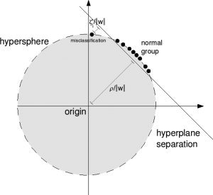
Illustration of one‐class SVM with an RBF kernel.

Applications of OC‐SVM can be found in image processing [Schölkopf et al., 2001], information retrieval [Manevitz and Yousef, 2002] and bioinformatics [Spinosa and Carvalho, 2005]. In medical research, Zhou et al. [ 2005] applied one‐class SVM in clinical applications focusing on the detection of tumor tissue in brain using magnetic resonance images. Gardner et al. [ 2006] used the technique in order to characterize seizures using intracranial EEG signals. In fMRI literature, applications OC‐SVM can be found in Hardoon and Manevitz [ 2005] and Song et al. [ 2007]. Further information, applications, details, and lectures about SVM and kernel methods can be found at http://www.csie.ntu.edu.tw/~cjlin/libsvm and http://www.videolectures.net/Top/Computer_Science/Machine_Learning/Kernel_Methods.

In general, the main goal of one‐class SVM in medical applications is to decide if a new subject does or does not belong to the class of “normal” subjects, or which subjects have patterns of behavior different from the majority of the population.

Normative Connectivity Database

The main proposal of this research is an approach combining both SPC and OC‐SVM. As described in previous sections, SPC can be used to identify underlying functional connectivity structures in the data. The connectivity network of a single subject can be described by a multivariate random variable representing the linkages intensities between the nodes. In addition, OC‐SVM is suitable to define normative databases from a multivariate perspective. Thus, assuming that fMRI data from a group of T subjects performing the same task is available, we propose the following approach:

• Step 1: Obtain group statistical parametric maps highlighting areas respondent to certain stimuli of interest

• Step 2: Select ROI, regarding the identification of network structure;

• Step 3: Extract individual BOLD time series representing the temporal variation within each ROI (it may be the local maxima of activation or cluster average time‐series);

• Step 4: Estimate individual functional connectivity structures by calculating SPC of ROIs time series. Thus, for each individual, a multivariate random variable of dimension K containing the links coefficients is observed;

• Step 5: Note that, T independent multivariate variables of dimension K are observed, and thus, OC‐SVM may be applied. In this context, the features are the partial correlation coefficients and the training examples are the individuals.

Data Acquisition

Forty‐three volunteers participated in this study. They had no history of neurological or psychiatric disease. The study was approved by the local ethical committee (CApPesq‐HC/FMUSP number 507/03) and subjects provided written informed consent in accordance with the Helsinki Declaration.

The subjects were scanned in a 1.5 T GE magnet, 33 mT/m (Milwaukee, USA) using a quadrature head coil. All subjects were instructed to maintain their heads still, and assisted in doing so using two adhesive ribbons on the forehead and lateral foam pads to minimize head motion without inducing discomfort.

Subjects were given a laterality questionnaire—the Edinburg inventory [Oldfield, 1971]. For each question, each subject had to select between the preferential left/right hand to perform a task (one point to the side selected), if he only uses the left/right hand (two points to the side) and whether it did not make a difference (one point for each side). The laterality index (LI) was calculated by computing

In summary, the LI varies from −1 to 1, where 1 describes a strongly right‐handed subject

The fMRI data set for each subject was obtained using a gradient‐echo echo‐planar sequence (EPI‐GRE) based on BOLD contrast. The acquisition parameters were: 5 mm thickness, 0.5 mm interslice gap, TR 2000 ms, TE 40 s, FOV 24 cm, matrix 64 × 64 mm², AC‐PC plane, 24 slices for each volume.

The experiment consisted of a visual working memory task, from the ICBM functional reference battery. This paradigm used an AB block design, during which the subject had to observe a cycle of abstract pictures followed by a single picture immediately after this cycle. He/she was asked to decide if this picture had been shown during that cycle or not. If it was repeated, the subject pressed the right button of a joystick, and if not, the left button. Each cycle was composed of a green circle at the start (presented for 400 ms), followed by a 50 ms blank screen, four different pictures (450 ms each), a red circle (400 ms) to indicate the end of the “encoding” picture cycle and then, after seeing a blank screen for 50 ms, a “test” picture is presented for 2,200 ms which they had to assess whether they had seen before. They were told to avoid using any kind of verbal label. In each “on” block there were five cycles. In each subject, the order of presentation of pictures and the order of cycles was random, but the same random order was used in all subjects. The participants were trained on the task prior to scanning, to become familiar with the five pictures, fully understand the task and improve performance. The stimuli were visually presented projected on a screen. The control condition consisted of arrowheads pointing to different positions, which were presented for 200 ms every 1,800 ms. The subjects were instructed to press the right button when the arrowhead was pointing to the right (>), the left button when it was pointing to the left (<), or do nothing when it was pointing up or down. The run was composed of six cycles. The experiment starts with an “off” block, which lasts 40 s. Each subsequent block lasts 28 s. Total number of images was 4,200 and the duration was 5 min and 56 s including 4 dummy acquisitions at the start of the experiment).

Image Processing

The fMRI datasets were processed for motion and slice time correction, spatially smoothed using a Gaussian kernel (FWHM = 9 mm) to improve signal to noise characteristics and normalized to the stereotatic space of Talairach and Tornoux [ 1988]. Activation maps were obtained using the fMRI software XBAM (http://www.brainmap.co.uk/xbam.htm), assuming a haemodynamic response described by a linear combinations of two Poisson functions with peak responses 4 and 8 s after stimulus onset. The group activation maps were obtained nonparametrically [Brammer et al., 1997; Bullmore et al., 1999].

The SPC was implemented in R platform (http://www.r-project.org) and OC‐SVM is available in the package e1071 (derived from LIBSVM at http://www.csie.ntu.edu.tw/~cjlin/libsvm).

RESULTS

The activated clusters in the memory task (cluster‐wise P‐value <0.05, see Fig. 2) are shown in Table I.

Figure 2.

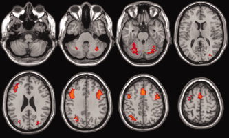
Group activation maps for the memory task experiment (p‐cluster <0.05).

Table I.

Areas significantly activated during the memory experiment (cluster‐wise P‐value <0.05)

Tal(x)	Tal(y)	Tal(z)	Side	BA	Brain region
−30	−71	−23	L	–	Cerebellum
29	−70	−29	R	–	Cerebellum
−25	−81	−7	L	18	Occipito‐parietal (V2,V3)
36	−59	42	R	19	Occipito‐parietal (V2,V3)
−43	19	26	L	47	Prefrontal cortex
47	11	31	R	44	Prefrontal cortex
4	15	42	L/R	24	Medial prefrontal cortex

Five clusters were selected as ROI: the right and left occipito–parietal visual cortex, the medial, right and left prefrontal cortex. For each subject, the average time series across voxels within the clusters were considered as the representative BOLD of the region. The application of detrending or any temporal filtering to this data was not found to be necessary based on analysis of the time series obtained.

The Spearman partial correlations between the BOLD signals of the five ROI's were then calculated separately for each individual. The functional connectivity network between the ROI's was then identified (see Fig. 3). The statistical significance of each link was then assessed by performing t tests (across subjects) assuming the null hypothesis of no partial correlation. All links were significant at a level of significance of 1% (Bonferroni multiple comparisons correction). However, Figure 3 shows that the links with the highest strengths are between the frontal areas and between ipsilateral visual and frontal areas. The intensities of these links were also estimated, for comparison, using Pearson's partial correlation. Nevertheless, the variance of Spearman's correlation was less than Pearson's in 8 of the 10 links, highlighting the robustness of the former and justifying its use.

Figure 3.

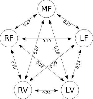
Estimated group connectivity network. The numbers in the arrows indicate values of Spearman partial correlation. (M/L/R)F: Medial, left and right frontal regions, respectively. (L/R)P: Left and right parietal cortex, respectively.

In the following, OC‐SVM with RBF kernel was applied to construct a normative database for the connectivity structure in this memory experiment. RBF is the most commonly choice for OC‐SVM kernel because it allows nonlinear classification, has an intuitive interpretation (see Fig. 1) and provides good results [Hardoon and Manevitz, 2005; Song et al., 2007]. As previously described, the parameter v can be seen as the upper bound for misclassification proportion, and considering the sample size, it was fixed at 0.2. The RBF parameter γ is related to the number of support vectors, and it was set aiming a number of support vector less than 30% of sample size (to avoid overfitting), resulting in γ = 0.01 with an error rate around 16.5% (i.e., observations at the tails of the distribution). Small values for ν and this accuracy rate were not chosen due to the relatively small number of examples available, which would lead to imprecise estimates. Parameter tuning using classical cross‐validation methods (leave‐one‐out, k‐fold,e etc) was not applied in this case, since it leads to overestimation of the misclassification rate (the sample size is relatively small and the observations in the tails are the most influential in hyperplane determination, mainly when the outliers are present in the data. This is an important point of concern, because fMRI experiments usually involve not more than twenty subjects per group and small numbers of outliers may have major effects. Using this approach, if the data of a new subject (BOLD time series of the ROIs') is available, one could decide, based on the estimated functional connectivity network, if this subject is or not from the population of the normative database. If more training examples were available, the rate of false positives may be decreased substantially.

Analysis of characteristics from subjects in the tails of the distribution (misclassified) was carried out to gain some insight on the origin of the factors underlying their extreme positions. The marginal kernel density estimate for each link is shown in Figure 4. The index and location of these misclassified subjects are also shown, and extreme observations (in the tails) are circled. It is important to highlight that the simple analysis of marginal distributions is not enough to achieve OC‐SVM criterion. In fact, OC‐SVM deals with multidimensional variables (in this case 10), and thus, the algorithm's decision is difficult to represent in a simple intuitive form. However, by its simplicity, the marginal analysis may provide some insight into the classification and interpretation of results. Note that for all misclassified observations, there is at least one connectivity link with an extreme value, compared to the rest of observations. In other words, these observations have at least one link different from the group pattern, which might be a plausible explanation for the misclassification.

Figure 4.

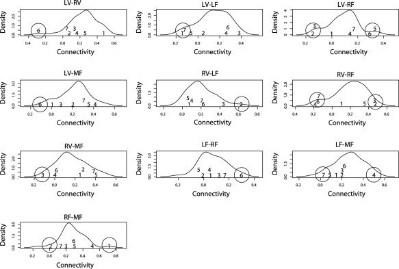
Kernel estimates of marginal densities for each feature variable (partial correlation). The numbers indicate the index and location of misclassified samples, which were considered in the tails of multivariate distribution (below p‐quantile). Extreme observations are highlighted with a circle.

The association between these differences in the connectivity structure and behavioral data is also a point of interest. Finding any behavioral characteristic that reflects this connectivity changes is the second target of this work. Figure 5 shows the kernel densities estimates for the laterality indices of all subjects. The index and location of misclassified subjects are also shown. Note that the laterality indices of these subjects lie in the tail of the distribution, that is, they are extreme values. In other words, subjects with extreme laterality indices show different functional networks, compared to the normal population. We are currently analyzing the implications of this finding, which may be an exciting way to look at behavior influences on the intersubject variability often found in fMRI datasets.

Figure 5.

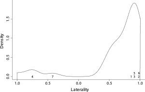
Kernel estimates density of laterality score in the data. The numbers indicate the index and location of misclassified samples using one‐class SVM.

DISCUSSION

Studies of functional integration are playing an important role in characterizing brain states and cognitive processes. To establish fMRI role in this setting, characterization of functional connectivity patterns and their correlates with behavioral data are critical. In this article, we suggest a combination of partial Spearman correlation coefficients and one‐class SVM, and show how this combination can be used to obtain a normative connectivity database in a memory experiment using fMRI. In addition, the correlations between subjects' classification and behavioral data show some quite consistent and interpretable results, suggesting that this approach can provide new information about the neural organization of brain functions and cognitive processing.

The multivariate profile of normal subjects extracted using one‐class SVM is described in terms of a multivariate probability distribution, instead of means or covariance matrices. This property is desirable, since the probability structure of non‐Gaussian or bimodal distributions cannot be adequately described only by their first two moments. In addition, after SVM is calibrated, new subjects can be classified as being normal or not by using the trained SVM. However, it is important to note that the specification of type I error (classification a subject as abnormal when he/she is normal) is associated with the sample size. A low P‐value for a type I error implies that only few observations laying outside the normal pattern will be used to estimate the desired quantile, leading to low precision. Thus, for an efficient false positive control, the type I error should be set according to the sample size.

In our study, the connectivity structure was identified using the Spearman partial correlation. Nevertheless, any approach that provides quantitative estimates of correlation strengths such as SEM, DCM, or multivariate autoregressive models (MAR) may be combined with one‐class SVM. In fact, the efficiency of the combination depends on the consistency and variability of the estimates across subjects. Generally, correlation measures are more consistent because of their simplicity and because they are only an index of synchronicity (functional connectivity), which is much less restrictive than “causality” or effective influences.

The experimental design is also important for obtaining reliable estimates of functional connectivity. For correlation analysis, block experiments may be preferable since they produce larger and stable BOLD effect sizes so that connectivity is driven by factors associated with the experimental design rather than “noise”. Even so, the method can be applied to event‐related paradigms, but the estimates of connectivity will depend on the reliability and signal to noise ratio of the experimentally related responses. On the other hand, the effectiveness of experimental design in the identification of neural networks depends on the approach adopted to estimate the connectivity links. Event related experiments are known to be adequate and efficient with DCM and MAR. In summary, one‐class SVM prediction power depends on the similarity of subjects' observations, thus, independently of the methods used to estimate the connectivity network, the paradigm should be set in order to minimize the variability between subjects.

The main limitations in applying one‐class SVM and SPC to obtain connectivity databases are related to the selection of ROI. In fact, the selection is necessary, since an fMRI volume is composed of a large number of voxels. Network estimation between all these voxels is feasible using pairwise correlations, principal component analysis or sparse vector autoregressive modelling [Valdes‐Sosa et al., 2005]. However, in these cases, the dimension of the feature vector would be large, with the inclusion of confounder variables, that is, connections with large variability across subjects and without interpretable relevance in the context of the task. Further, the inclusion of variables decreases the estimates of partial correlation, increases its variances and makes the interpretation of the results complex. For this reason, we suggest the inclusion only of those regions comprising the neural networks related to the paradigm under investigation. A second limitation, related to the latter, is that despite the fact of being able to identify abnormal subjects, one‐class SVM does not explicitly indicate which of characteristics that they possess lead to this abnormality. Some possible reasons can be found in the analysis of each network connection separately (as in Fig. 4). Nevertheless, the classification may be possibly related to multivariate properties of the data, and thus, univariate analysis of a large set of variables can be complex or not informative at all.

Future projects involve the application of the proposed approach to obtain specific pathologic databases. Normative databases of healthy individuals are useful to decide if a subject is healthy or not. However, if a subject is classified as being non‐normal, treatment indications are not always clear. On the other hand, one may obtain a pathologic database of respondents to a specific treatment. Thus, if an individual suffers from a disease (Parkinson, depression, Alzheimer, etc) and he/she is classified as being respondent to a certain therapy, there is evidence that this treatment is adequate for him/her. In addition, OC‐SVM may be more suitable than two classes SVM in cases when some patients demonstrate profiles similar to normal ones. Thus, supervised learning may fail in this case, but one‐class SVM would still be consistent to detect patients with abnormal profiles.

In conclusion, clinical applications of fMRI are still at research stage and the development of new technologies to extract profiles from normative databases will be essential for their wider use.

REFERENCES

- Alashwal H,Deris S,Othman RM ( 2006): One‐class support vector machines for protein‐protein interactions prediction. Int J Biomed Sci 1: 120–127. [Google Scholar]
- Bandettini P ( 2007): Functional MRI today. Int J Psychophysiol 63: 138–145. [DOI] [PubMed] [Google Scholar]
- Biswal B,Yetkin FZ,Haughton VM,Hyde JS ( 1995): Functional connectivity in the motor cortex of resting human brain using echo‐planar MRI. Magn Reson Med 34: 537–541. [DOI] [PubMed] [Google Scholar]
- Brammer MJ,Bullmore ET,Simmons A,Williams SC,Grasby PM,Howard RJ,Woodruff PW,Rabe‐Hesketh S ( 1997): Generic brain activation mapping in functional magnetic resonance imaging: a nonparametric approach. Magn Reson Imaging 15: 763–770. [DOI] [PubMed] [Google Scholar]
- Bullmore ET,Suckling J,Overmeyer S,Rabe‐Hesketh S,Taylor E,Brammer MJ ( 1999): Global, voxel, and cluster tests, by theory and permutation, for a difference between two groups of structural MR images of the brain. IEEE Trans Med Imaging 18: 32–42. [DOI] [PubMed] [Google Scholar]
- Burges CJC ( 1998): A Tutorial on Support Vector Machines for Pattern Recognition. Boston: Kluwer Academic. [Google Scholar]
- Campbell C,Bennett K ( 2000): A linear programming approach to novelity detection. In Advances in Neural Information Processing Systems 13: Proceedings of the 2000 Conference. MIT‐Press.
- Friston KJ,Harrison L,Penny W ( 2003): Dynamic causal modelling. Neuroimage 19: 1273–1302. [DOI] [PubMed] [Google Scholar]
- Gardner AB,Krieger AM,Vachtsevanos G,Litt B ( 2006): One‐class novelty detection for seizure analysis from intracranial EEG. J Mach Learn Res 7: 1025–1044. [Google Scholar]
- Hardoon DR,Manevitz LM ( 2005): fMRI Analysis via One‐class Machine Learning Techniques. International Joint Conferences on Artificial Intelligence. Scotland: Edinburgh. pp 1604–1605.
- Kriegl JM,Arnhold T,Beck B,Fox T ( 2005): A support vector machine approach to classify human cytochrome P450 3A4 inhibitors. J Comput Aided Mol Des 19: 189–201. [DOI] [PubMed] [Google Scholar]
- McIntosh AR ( 1999): Mapping cognition to the brain through neural interactions. Memory 7: 523–548 (Review). [DOI] [PubMed] [Google Scholar]
- Manevitz LM,Yousef M ( 2002): One‐class svms for document classification. J Mach Learn Res 2: 139–154. [Google Scholar]
- Marrelec G,Krainik A,Duffau H,Pelegrini‐Issac M,Lehericy S,Doyon J,Benali H ( 2006): Partial correlation for functional brain interactivity investigation in functional MRI. Neuroimage 32: 228–237. [DOI] [PubMed] [Google Scholar]
- Marrelec G,Horwitz B,Kim J,Pélégrini‐Issac M,Benali H,Doyon J ( 2007): Using partial correlation to enhance structural equation modeling of functional MRI data. Magn Reson Imaging 25: 1181–1189. [DOI] [PubMed] [Google Scholar]
- Mitchell TM,Hutchinson R,Niculescu RS,Pereira F,Wang X,Just M,Newman S ( 2004): Learning to decode cognitive states from brain images. Mach Learn 57: 145–175. [Google Scholar]
- Mourao‐Miranda J,Bokde AL,Born C,Hampel H,Stetter M ( 2005): Classifying brain states and determining the discriminating activation patterns: Support vector machine on functional MRI data. Neuroimage 28: 980–995. [DOI] [PubMed] [Google Scholar]
- Mourao‐Miranda J,Reynaud E,McGlone F,Calvert G,Brammer M ( 2006): The impact of temporal compression and space selection on SVM analysis of single‐subject fMRI data. Neuroimage 33: 1055–1065. [DOI] [PubMed] [Google Scholar]
- Mourao‐Miranda J,Friston KJ,Brammer M ( 2007): Dynamic discrimination analysis: a spatial‐temporal SVM. Neuroimage 36: 88–99. [DOI] [PubMed] [Google Scholar]
- Oldfield RC ( 1971): The assessment and analysis of handedness: The Edinburgh inventory. Neuropsychologia 9: 97–113. [DOI] [PubMed] [Google Scholar]
- Ogawa S,Lee TM,Kay AR,Tank DW ( 1990): Brain magnetic resonance imaging with contrast dependent on blood oxygenation. Proc Natl Acad Sci USA 87: 9868–9872. [DOI] [PMC free article] [PubMed] [Google Scholar]
- Peltier SJ,Noll DC ( 2001): T2* Dependence of low frequency functional connectivity. Neuroimage 16: 985–992. [DOI] [PubMed] [Google Scholar]
- Schölkopf B,Platt JC,Shawe‐Taylor JS,Smola AJ,Williamson RC ( 2001): Estimating the support of a high‐dimensional distribution. Neural Comput 13: 1443–1471. [DOI] [PubMed] [Google Scholar]
- Schölkopf B,Smola AJ ( 2002): Learning With Kernels: Support Vector Machines,Regularization, Optimization and Beyond. Cambridge, MA: MIT Press. [Google Scholar]
- Song X,Iordanescu G,Wyrwicz A ( 2007): One‐class machine learning for brain activation detection. IEEE Conference on Computer Vision and Pattern Recognition. United States: Minneapolis. pp 1–6.
- Spinosa EJ,Carvalho AC ( 2005): Support vector machines for novel class detection in Bioinformatics. Genet Mol Res 4: 608–615. [PubMed] [Google Scholar]
- Talairach J,Tournoux P ( 1988): Co‐planar Stereotaxic Atlas of the Human Brain. New York: Thieme. [Google Scholar]
- Tax D,Duin R ( 1999): Data domain description by support vectors In: Veleysen M,editor. Proceeding of ESANN. Brussels: D. Facto Press; pp 251–256. [Google Scholar]
- Tsirigos A,Rigoutsos I ( 2005): A sensitive, support vector machine method for the selection of horizontal gene transfers in viral, archaeal and bacterial genomes. Nucleic Acids Res 33: 3699–3707. [DOI] [PMC free article] [PubMed] [Google Scholar]
- Valdes‐Sosa PA,Sanchez‐Bornot JM,Lage‐Castellanos A,Vega‐Hernandez M,Bosch‐Bayard J,Melie‐Garcia L,Canales‐Rodriguez E ( 2005): Estimating brain functional connectivity with sparse multivariate autoregression. Philos Trans R Soc Lond B Biol Sci 360: 969–981. [DOI] [PMC free article] [PubMed] [Google Scholar]
- Vapnik V ( 1995): The Nature of Statistical Learning Theory. New York: Springer‐Verlag. [Google Scholar]
- Xiong J,Parsons LM,Gao J,Fox PT ( 1999): Interregional connectivity to primary motor cortex revealed using MRI resting state images. Hum Brain Mapp 8: 151–156. [DOI] [PMC free article] [PubMed] [Google Scholar]
- Wang X,Hutchinson R,Mitchell TM ( 2003): Training fMRI classifiers to discriminate cognitive states across multiple subjects. The 17th Annual Conference on Neural Information Processing Systems. Canada: Vancouver.
- Wang Z,Childress AR,Wang J,Detre JA ( 2007): Support vector machine learning‐based fMRI data group analysis. Neuroimage 36: 1139–1151. [DOI] [PMC free article] [PubMed] [Google Scholar]
- Zhou J,Chan KL,Chong VFH,Krishnan SM ( 2005): Extraction of brain tumor from MR images using one‐class support vector machines. In the Proceedings of 2005 IEEE Engineering in Medicine and Biology. China: Shanghai. [DOI] [PubMed]