Multivariate Granger causality analysis of fMRI data

Abstract

This article describes the combination of multivariate Granger causality analysis, temporal down‐sampling of fMRI time series, and graph theoretic concepts for investigating causal brain networks and their dynamics. As a demonstration, this approach was applied to analyze epoch‐to‐epoch changes in a hand‐gripping, muscle fatigue experiment. Causal influences between the activated regions were analyzed by applying the directed transfer function (DTF) analysis of multivariate Granger causality with the integrated epoch response as the input, allowing us to account for the effects of several relevant regions simultaneously. Integrated responses were used in lieu of originally sampled time points to remove the effect of the spatially varying hemodynamic response as a confounding factor; using integrated responses did not affect our ability to capture its slowly varying affects of fatigue. We separately modeled the early, middle, and late periods in the fatigue. We adopted graph theoretic concepts of clustering and eccentricity to facilitate the interpretation of the resultant complex networks. Our results reveal the temporal evolution of the network and demonstrate that motor fatigue leads to a disconnection in the related neural network. Hum Brain Mapp, 2009. © 2008 Wiley‐Liss, Inc.

INTRODUCTION

The role of networks in brain function has been increasingly recognized over the past decade [Friston et al., 1993; Sporns et al., 2004]. In functional neuroimaging, brain networks are primarily studied in terms of functional connectivity (defined as temporal correlations between remote neurophysiologic events) and effective connectivity (defined as the causal influence one neuronal system exerts over another) [Friston, 1995]. Though the two prominent approaches to characterizing effective connectivity—structural equation modeling [McIntosh et al., 1994) and dynamic causal modeling [Friston et al., 2003]—have their advantages and disadvantages, neither of them incorporate information on temporal precedence, which may be considered as a necessary condition for causality. Also, these techniques require an a priori specification of an anatomical network model and are therefore best suited to making inferences on a limited number of possible networks. Recently, an exploratory structural equation model approach that does not require prior specification of a model was described [Zhuang et al., 2005]. However with increasing number of regions of interest, its computational complexity becomes intractable and the numerical procedure becomes unstable. These disadvantages can largely be circumvented by methods which are based on the cross‐prediction between two time series such as Granger causality [Granger, 1969].

With fMRI data, recent studies have applied Granger causality analysis between a target region of interest (ROI) and all other voxels in the brain to derive Granger causality maps [Abler et al., 2006; Goebel et al., 2003; Roebroeck et al., 2005]. A major limitation of applying the target ROI based approach to neuroimaging data is that it is a bivariate method and ignores interactions between other ROIs in the underlying neuronal network leading to an oversimplification of the multivariate neuronal relationships that exist during the majority of cognitive tasks. Simulations by Kus et al. [2004] have shown that a complete set of observations from a process have to be used to obtain causal relationships between them and that pair‐wise estimates may yield incorrect results. To date, multivariate measures of Granger causality have been largely limited to electrophysiological data [Blinowska et al., 2004; Ding et al., 2000; Kaminski et al., 2001; Kus et al., 2004] although multivariate autoregressive models have been used to infer functional connectivity from fMRI data [Harrison et al., 2003]. We have previously presented preliminary forms of the study described here [Deshpande et al., 2006a, b].

A critical consideration for fMRI data is the limitations imposed by the hemodynamic response. The fMRI response is dictated by the sluggish hemodynamic response, which is believed to be spatially dependent [Aguirre et al., 1998; Handwerker et al., 2004; Silva et al., 2002]. Given that the hemodynamic response takes 6–10 s, Granger causality analysis applied to the measured raw time series sampled with a TR on the order of a second may be contaminated by regional differences in the hemodynamic response. We alleviate the effect of spatially varying hemodynamic delay by focusing on the causal relationships at a temporal scale much coarser than the hemodynamic response. Neuronal processes such as fatigue, learning, and habituation evolve slower than the hemodynamic response and are amenable to a coarse temporal scale causal analysis.

Another consideration is that multivariate causality relationships can be difficult to interpret and to compare across data sets. With several anatomical regions included in a network, the possible number of interconnections between them increases quadratically. The complexity of the problem is further increased by our desire to characterize the temporal evolution of these network interactions. Graph theoretic concepts are well suited to represent the information present in these networks. Graphical representations for fMRI‐derived causal neuronal networks were introduced recently in the context of studying unmeasured latent variables in effective connectivity analysis [Eichler, 2005]. The utility of graphical models in characterizing the topology of large networks has been demonstrated in the case of anatomical networks in macaques [McIntosh et al., 2006], and functional networks obtained from MEG [Stam, 2004] and EEG [Fallani et al., 2006; Sakkalis et al., 2006]. In the present study, we have used the graphical representation for effective characterization of the network topology. In addition to utilizing concepts such as clustering [Fallani et al., 2006; Sakkalis et al., 2006; Stam, 2004], we introduce the application of eccentricity analysis to determine the ROIs having a major influence on the network.

In this work, we have adapted the directed transfer function (DTF) which was recently introduced as a causal multivariate measure for EEG [Kus et al., 2004]. The DTF is based on Granger causality, but is rendered in a multivariate formulation [Blinowska et al., 2004] and hence is effective in modeling the inherent multivariate nature of neuronal networks. For our application, we used the product of the non‐normalized DTF and partial coherence to emphasize the direct connections and de‐emphasize mediated influences. This procedure has been shown to be robust [Kus et al., 2004] although equally good options such as conditional Granger causality exist [Chen et al., 2006]. Using an extended period of fMRI data collected during a fatigue experiment [Peltier et al., 2005], we extracted the area under each epoch to form a summary time series which captures the epoch‐to‐epoch variation. The rationale was that this is more likely to reflect the physiological process of fatigue and also alleviates the effect of the spatially varying hemodynamic delay. This fact was substantiated using simulations. Further, we investigated the changes in the dynamics of the networks as the subjects progressively fatigued, demonstrating the utility of this approach.

MATERIALS AND METHODS

MRI Data Acquisition and Preprocessing

Ten healthy right‐handed male subjects performed a prolonged motor task while they underwent functional magnetic resonance imaging in a 3T Siemens Trio (Siemens AG, Berlin, Germany). Informed consent was obtained prior to scanning and the procedure was approved by the internal review board at Emory University. The subjects performed repetitive right‐hand contractions at 50% maximal voluntary contraction (MVC) level by gripping a bottle‐like device [Liu et al., 2002]. Online measurement of handgrip force was accomplished by a pressure transducer connected to the device through a nylon tube filled with distilled water. For each subject, the target level of 50% MVC was calculated based on the maximal grip force measured at the beginning of the experiment. Visual cues (a rectangular pulse whose profile matched the amplitude and duration of the handgrip contraction) were generated by a waveform generator and projected onto the screen above the subject's eye in the magnet to guide the subjects in performing the contractions. Each contraction lasted 3.5 s, followed by a 6.5 s intertrial interval (ITI). The total fatigue task comprised of 120 contractions lasting 20 min. After the completion of the task, the level of muscle fatigue was determined by measuring the MVC handgrip force. The choice of 50% MVC level was made so as to fatigue the muscles in ∼10–15 min for the given length of contraction and ITI. Echo planar imaging (EPI) data was obtained with the following scan parameters: Thirty 4‐mm slices (no gap) covering from the top of the cerebrum to the bottom of the cerebellum, 600 volumes, repetition time (TR) of 2 s, echo time (TE) of 30 ms, a flip angle (FA) of 90°, and an in‐plane resolution of 3.44 × 3.44 mm².

The data analysis for activation detection was carried out using Brainvoyager™ 2000 (Ver 4.9 © Rainer Goebel and Max Planck Society, Maastricht, The Netherlands. http://www.brainvoyager.com). Two subjects were excluded from the analysis because of excessive head motion. Subsequent to motion and slice scan time correction, a reference waveform derived based on the activation paradigm (Fig. 1) was correlated with each detrended voxel time series to produce activation maps (Fig. 2). The correspondence of the activation paradigm with a time series from the primary motor area is illustrated in Figure 1. As shown in Figure 2, six ROIs—contralateral (left) primary motor (M1) cortex, primary sensory cortex (S1), premotor area (PM), ipsilateral (right) cerebellum (C), supplementary motor area (SMA), and parietal area (P)—were identified from the activation maps, and ROI specific average time courses were obtained. Because of the overlap of activations in M1 and S1, these areas were delineated based on the location of central gyrus [Yousry et al., 1997] by assigning the activations in the precentral gyrus as M1 and that in the postcentral gyrus as S1. SMA activation was taken to be medial and the parietal activation included both medial and contra‐lateral activations in the posterior parietal cortex.

Figure 1.

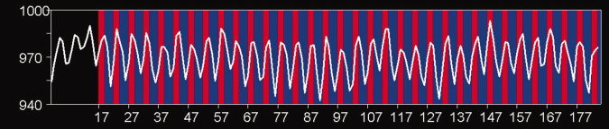
A time series from M1 overlaid on the activation paradigm. Red: 3.5 s contraction. Blue: 6.5 s intertrial interval. [Color figure can be viewed in the online issue, which is available at www.interscience.wiley.com.]

Figure 2.

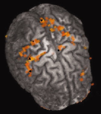
A sample activation map obtained from the fatigue motor task showing the regions of interest. ▪ SMA, ▴M1, * S1, ♥ P, ◂ PM.

To investigate fatigue induced causal influences, the area under the time course of each epoch was calculated as a summary measure and a corresponding summary time series was derived from the mean time series for each ROI (Fig. 3). An epoch was defined as the duration containing the contraction time and intertrial interval. The underlying hemodynamic response in each epoch corresponded to one contraction. Three nonoverlapping segments from the summary time series, each containing 40 points, was input into the multivariate Granger causality analysis. The use of these windows allowed us to investigate the temporal dynamics of the network.

Figure 3.

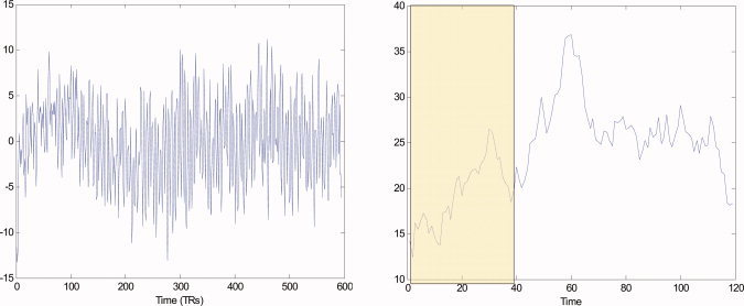
Left: Original fMRI time series. Right: Summary time series (yellow patch shows the first time window). [Color figure can be viewed in the online issue, which is available at www.interscience.wiley.com.]

Simulations

The purpose of the simulations was to show that hemodynamic confounds can overwhelm long term effects, leading to erroneous results and this confound can be eliminated by analyzing the summary time series. Two time series, R₁ and R₂, were simulated by assuming an event‐related paradigm consisting of 120 trials with an epoch duration of 20 s. Each event was assumed to lead to a HRF defined by two Gamma functions [Friston et al., 1999] with the following parameters: sampling interval = 2 s, dispersion of response = 1 s, dispersion of undershoot = 1 s, delay of response (relative to onset) = 6 s, delay of undershoot (relative to onset) = 10 s, ratio of response to undershoot = 6, length of kernel = 20 s. The HRF for R₁ was assumed to be 1 s behind that of R₂ (i.e., R₂ leads R₁). The peak amplitudes for the trials in R₁ and R₂ were modulated by slowly varying sinusoids, denoted by A₁ and A₂, with A₁ leading A₂ by one epoch. Because an epoch is 20 s long, R₁ leads R₂ inspite of the 1 s hemodynamic lead R₂ has over R₁. Gaussian noise (SNR = 0, 5, 10, and 100, 500 realizations each) was added to the simulated signals to test the effect of random noise in the system. Granger causality analysis was applied to raw time series, R₁ and R₂, and the summary time series obtained by integrating each epoch, C₁ and C₂. Because C₁ and C₂ are proportional to A₁ and A₂, respectively, C₁ leads C₂.

Multivariate Granger Causality Analysis

The principle of Granger causality is based on the concept of cross prediction. Accordingly, if incorporating the past values of time series X improves the future prediction of time series Y, then X is said to have a causal influence on Y [Granger, 1969]. In the case of any two time series X and Y, the efficacy of cross‐prediction could be inferred either through the residual error after prediction [Roebroeck et al., 2005] or through the magnitude of the predictor coefficients [Blinowska et al., 2004]. Both approaches are equivalent and the analytical relationship between them is given by Granger [1969]. In this section, we describe the multivariate model of Granger causality used in this study.

The Granger causality analysis was accomplished using custom software written in MATLAB (The MathWorks Inc, Massachusetts). A multivariate autoregressive (MVAR) model was constructed from the summary time series of the ROIs. In the following, an italic capital letter represents a matrix with components corresponding to the ROIs and the variable in the parenthesis indicates either time or temporal frequency. Let X(t) = (x ₁(t),x ₂(t),…x_k(t))^T be the data matrix and x_k correspond to the time series obtained from the kth ROI. The MVAR model with model parameters A(n) of order p is given by

(1)

where E(t) is the vector corresponding to the residual error. This form of MVAR is analytically proven to have a unique solution [Caines et al., 1975; Granger, 1969]. Akaike information criterion (AIC) was used to determine the model order [Akaike, 1974]. Equation (1) can be rewritten as follows

(2)

Equation (2) was transformed to the frequency domain resulting in

(3)

We designate and A as the matrix corresponding to elements a_ij. Here, δ_ij is the Dirac‐delta function which is one when i = j and zero elsewhere. Also, , where k is the total number of ROIs. Note that time domain matrices are represented by bold letters and their frequency domain counterparts are denoted by capital letters in normal font.

(4)

(5)

The transfer matrix of the model, H(f), contains all the information about the interactions between the time series and h_ij(f), the element in the ith row and jth column of the transfer matrix, is referred to as the non‐normalized DTF [Kus et al., 2004] corresponding to the influence of ROI j onto ROI i. Least squares estimation [Tyraskis et al., 1985] was used to solve for the prediction coefficients. This procedure imposes a theoretical constraint that the number of data points in each time series be more than the number of MVAR parameters to be estimated (which is the square of the number of time series for a first order model) [Kus et al., 2004; Tyraskis et al., 1985].To emphasize direct connections and de‐emphasize mediated influences, H(f) was multiplied by the partial coherence between ROIs i and j to obtain direct DTF (dDTF) [Korzeniewska et al., 2003; Kus et al., 2004]. Simulations provided by Kus et al. and Korzeniewska et al. prove that dDTF is a robust measure capable of de‐emphasizing mediated influences. To calculate the partial coherence, we first computed the cross‐spectra using

(6)

where V is the variance of the matrix E(f) and the asterisk denotes transposition and complex conjugate. The partial coherence between ROIs i and j is then given by

(7)

where the minor M_ij(f) is defined as the determinant of the matrix obtained by removing the ith row and jth column from the matrix S.

The partial coherence between a pair of ROIs indicates the association between them when the statistical influence of all other ROIs is discounted. It lies in the range [0, 1] where a value of zero indicates no direct association between the ROIs. The direct DTF (dDTF) was obtained as the sum of all frequency components of the product of the non‐normalized DTF and partial coherence as given in the equation below.

(8)

dDTF as defined above emphasizes the direct connections between ROIs. Working in the frequency domain offers the advantage of uncovering interactions in specific frequency bands. In our data, we did not observe distinct frequency specific patterns except that Granger causality remained high in the lower frequencies and decreased with increasing frequency. This is to be expected considering the fact that the summary time series had higher spectral energy in the low frequency band. Hence we summed all the frequency components to obtain one dDTF value for every connection. Methodologically, spectral methods have been shown to be more robust to deviations from the stationarity assumption [Granger, 1964].

It is to be noted that unlike previously reported studies [Blinowska et al., 2004; Kaminski et al., 2001; Kus et al., 2004], we avoided normalizing DTF so as to allow direct comparison between the absolute values of the strengths of influence. Normalization of DTF with respect to inflows into any ROI as in Kus et al. [Kus et al., 2004] would make such a comparison untenable. As described in the previous subsection, the calculation of dDTF was carried out using the summary time series in three nonoverlapping windows so as to investigate the temporal dynamics of the network. In addition, connectivity was also computed using the raw time series for comparison.

Statistical Significance Testing

Analytical distributions of multivariate Granger causality are not established because they are said to have a highly nonlinear relationship with the time series data [Kaminski et al., 2001]. Therefore, to assess the significance of the Granger causality reflected by dDTF, we employed surrogate data [Kaminski et al., 2001; Kus et al., 2004; Theiler et al., 1992] to obtain an empirical null distribution. The original time series was transformed into the frequency domain and their phase was randomized so as to be uniformly distributed over (−π, π) [Kus et al., 2004]. Subsequently, the signal was transformed back to the time domain to generate the surrogate data. This procedure ensured that the surrogate data possessed the same spectrum as the original data but with the causal phase relations destroyed. dDTF was calculated between the surrogate data time series representing each ROI. Null distributions were derived for all possible connections between the ROIs, in each time window and for every subject, by repeating the above procedure 2,500 times. Therefore, corresponding to six ROIs (we had 30 possible links between the ROIs) and three time windows, a total of 90 null distributions were generated per subject. For each connection, the actual dDTF was compared with its corresponding null distribution to derive a P‐value. To obtain group significance inference, the P‐values from individual subjects were combined using Fisher's method [Fisher, 1932] to obtain a single P‐value. This procedure was repeated for each connection in the three temporal windows to obtain significant connectivity networks. Using a Jarque‐Bera test for goodness‐of‐fit to a normal distribution, the distribution of path coefficients within a single time window and the distribution of the difference in path coefficients were determined to be normal. To assess the significance of the change in path coefficients across different time windows, a paired t‐test was performed between windows 1 and 2 and between 2 and 3. The significance values were controlled for multiple comparisons using Bonferroni correction [Miller, 1991].

Graph Analysis

The causal influences between the ROIs in a network could in principle be represented as a weighted directed graph, whose weights are represented by the dDTF value for the corresponding link between the ROIs, the direction of the link being the direction of causal influence and the ROIs themselves representing the vertices (or nodes) of the network. As mentioned in the introduction, this type of representation has been used to characterize network topology of causal functional networks obtained from MEG data [Stam, 2004] and EEG [Fallani et al., 2006; Sakkalis et al., 2006]. In this study, we focus on clustering and eccentricity. Although clustering has been used previously [Fallani et al., 2006; Sakkalis et al., 2006; Stam, 2004], we have adopted the concept of eccentricity from graph theory [Edwards, 2000] and have shown its relevance in interpreting the resultant networks.

Mathematical representation of a graph

A graph G is mathematically represented in the form of a sparse matrix called the adjacency matrix [Skiena, 1990]. The adjacency matrix of the directed graph is a matrix with rows and columns labeled by graph vertices (v), with the dDTF value corresponding to the influence from v_j to v_i in the position (v_i,v_j).

Clustering coefficient

One of the most important aspects of the topology of a network is the role of the nodes as either drivers of other nodes or being driven by other nodes. This is assessed by the total strength of causal influence that is emanating from or incident on the node. Correspondingly, cluster‐in and cluster‐out coefficients [Watts et al., 1998] are defined as,

(9)

(10)

where k = 6 is the number of nodes in the network. Basically, C _in of a node is the sum of all the corresponding columns of G and C _out is the sum of all corresponding rows. While calculating clustering coefficients from the fatigue data, the mean dDTF averaged over the subjects were used as entries in the matrix G. Also, the analysis was carried out separately for each of the three temporal windows.

Eccentricity

The eccentricity E(v) of a graph vertex v in a connected graph G is the maximum geodesic distance between v and any other vertex u of G. The geodesic distance between two vertices in a weighted graph is the sum of the causal influences along the shortest path connecting them. We used the Floyd‐Warshall algorithm for solving the all‐pairs shortest path problem [Cormen et al., 2001] to the find the shortest path between any pairs of nodes. Given that graph distance is measured in terms of the strength of causal influence, the shortest path between two nodes indicates the path along which maximum causal influence is exerted. Eccentricity is related to the individual influence of a vertex on the overall network performance [Skiena, 1990]. A vertex v is said to have a major influence on the network performance if it has the maximum E(v) among all vertices in the graph. Such a vertex, termed the major node, wields maximum influence on network behavior. The major nodes in each time window were ascertained to infer the changing roles of brain regions.

RESULTS

Simulations

Table I lists the results obtained from the simulations. Except when SNR = 0, dDTF derived using integrated time series reflects the correct connectivity (C₁→C₂). In contrast, the connectivity derived using the raw time series (R₂→R₁) is incorrect and appears to be more bidirectional as opposed to unidirectional in case of the integrated time series for lowers SNRs. At high SNRs, the ratio of dDTF along the direction of minor influence to that along the major influence is lower with the integrated time series than with the raw time series.

Table I.

Simulation results for raw time series and coarse time series

Connection	SNR = 0	SNR = 5	SNR = 10	SNR = 100
Raw time series
R1→R2	0.03 ± 0.04	0.08 ± 0.09	0.7 ± 0.2	3.7 ± 0.1
R2→R1	0.05 ± 0.08	6.2 ± 1.0	8.5 ± 1.1	13.9 ± 0.5
Coarse time series
C1→C2	0.4 ± 0.6	20 ± 3.4	28.1 ± 2.9	38 ± 0.8
C2→C1	0.4 ± 0.4	0.6 ± 0.5	2.1 ± 0.9	6.8 ± 0.3

Here, the connectivity values indicate the dDTF (summed connectivity over the whole spectra) as well as its standard deviation over all the realizations. C₁ drives C₂ and R₁ drives R₂ by construction. The model obtained by coarse time series is more accurate than the one obtained by the raw time series confounded by hemodynamics.

Behavioral Data and Preprocessing

There was a significant decrease (P < 0.002) in hand grip force measured after the motor task as compared to before the task, indicating that significant muscle fatigue had occurred. Of the eight subjects selected for analysis, behavioral data was not available for two subjects due to technical difficulties. In the rest of the six subjects, the decrease in hand grip force was 29% ± 11% [Peltier et al., 2005]. Figure 2 shows a sample activation map obtained by correlating the fMRI time series with the reference waveform and the ROIs selected for further analysis. A representative summary time series and the original time series that it is derived from are shown in Figure 3. It can be seen that the summary time series captures the slow epoch‐to‐epoch variation and in this particular case represents an initial increase and subsequent stagnation of the epoch response.

Multivariate Granger Causality

A model order of one was assigned based on the Akaike information criterion [Akaike, 1974]. Because a single time point in the summary time series corresponds to the area under the corresponding epoch, the resulting MVAR model represents epoch‐to‐epoch prediction. The temporal variation of the significance values α (α = 1−P) for connections between all pairs of ROIs is shown in Figure 4. The links that passed the significance threshold of α = 0.95 are represented by the bars in red while the connections that did not pass the threshold are shown as green bars. The network representation of the results in Figure 4 is shown in Figure 5, where the significant connections are shown as solid lines with their width reflecting the statistical significance of the influence. It is to be noted that the absence of a connection does not necessarily imply that there is no causal influence between the corresponding ROIs. A more lenient threshold or additional statistical power might render an insignificant connection significant. The thresholded difference networks between windows 1 and 2 and between windows 2 and 3 are shown in Figure 6, illustrating the shift in connectivity patterns. As a comparison, the networks obtained from raw time series (using a model order one as determined by the application of AIC to raw time series) are depicted in Figure 7.

Figure 4.

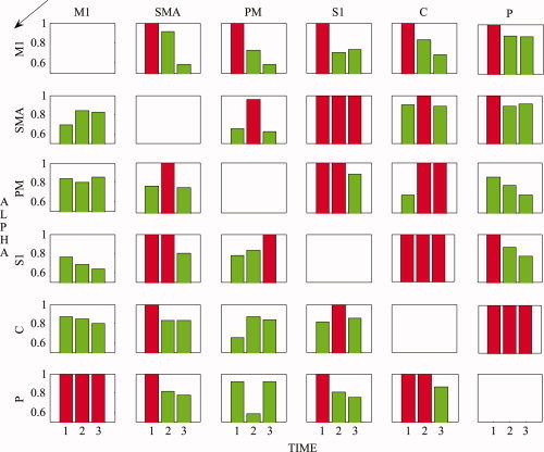
The temporal variation of significance value α (α = 1−P) for all possible connections between the ROIs. The direction of influence, as indicated by the black arrow, is from the columns to the rows. The red bars indicate the connections that passed the significance threshold of α = 0.95 and the green ones that did not. [Color figure can be viewed in the online issue, which is available at www.interscience.wiley.com.]

Figure 5.

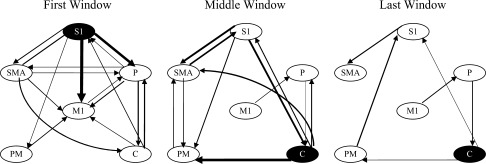
A network representation of Figure 4. The significant links are represented as solid arrows and the P‐value of the connections are indicated by the width of the arrows. The major node in each window is also indicated as dark ovals.

Figure 6.

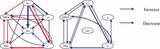
Thresholded difference networks. Left: window 1–window 2. Right: window 2–window 3. Red indicates positive difference whereas blue indicates negative difference.

Figure 7.

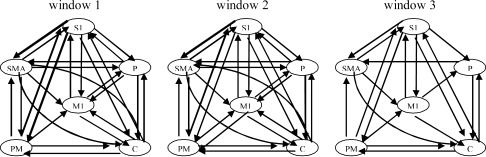
Networks obtained from raw time series for the three windows. The significant links (P <0.05) are represented as solid arrows and the P‐value of the connections are indicated by the width of the arrows.

The computational times for different components of the implementation on a 2.7 GHz Pentium 5 machine were as follows. Calculating the summary time series for 600 volumes took 2.93 s while dDTF calculation for each time window took 1.28 s. The total runtime of the code will depend on the number of times dDTF is calculated on the surrogate time series.

Graph Analysis

Clustering coefficients

Table II lists C _in and C _out for the three windows. In the first window, M1 was predominantly driven while S1 was a strong driver. The other areas had a dual role in the sense that they both received and transmitted information. In the second window, S1 and cerebellum were strong drivers. In the third window, while S1 and cerebellum remained to be the main drivers, the absolute value of the coefficients decreased for all ROIs, indicating a reduction of network connectivity. This reduction, also evident in Figure 5, indicates that as muscles fatigued, the connections in the motor network decreased.

Table II.

Cluster‐in and cluster‐out coefficients for all ROIs for the three windows

		M1	SMA	PM	S1	C	P
Window‐1	C in	19	15	7	9	16	11
	C out	8	13	7	25	10	13
Window‐2	C in	15	21	15	9	16	8
	C out	8	14	11	23	18	10
Window‐3	C in	11	13	9	9	15	8
	C out	7	8	9	18	14	9

Eccentricity

The primary sensory area was the major node in the first window, while the cerebellum was the major mode in the second and third windows. This is schematically represented in Figure 5 where the major nodes are marked in black. This result indicates that S1 wielded maximum influence on the network in the first window, and the dominance of influence shifted to the cerebellum in the second and third windows.

DISCUSSION

The simulation results support the argument that Granger causality analysis could be confounded by hemodynamic variability which could arise due to a multitude of factors [Aguirre et al., 1998; Handwerker et al., 2004; Silva et al., 2002]. In the simulation, this is demonstrated by the fact that the simulated connections were incorrectly identified by Granger analysis of raw time series but correctly identified by analyzing the summary time series. The analysis of summary time course is robust in the presence of Gaussian noise. Fatigue is a slowly evolving process [Liu et al., 2002a,b] and the causal influences underlying fatigue can be assumed to lie on a coarser time scale. Based on the simulation, it is prudent to use the summary time series in the MVAR instead of the raw time series to recover the long term causal influences due to fatigue. An MVAR of summary time series represents epoch‐to‐epoch evolution. Each epoch represents a contraction and the area under it represents the net activity of an ROI due to the contraction. Hence, epoch‐to‐epoch causal influence is interpreted as predicting the activities for future contractions based on those for the current contraction.

According to Wei, subsampling weakens the magnitude of Granger causality, but preserves the direction and temporal aggregation may cause spurious Granger causality. Their conclusion was based on the assumption that the true causal influence is at a finer time scale than the sampling resolution [Wei, 1982]. In contrast, given that fatigue is a slowly evolving process, the long‐term causal influences corresponding to the underlying neurophysiological processes involving fatigue are occurring at a coarser time scale than the sampling resolution. Therefore Wei's conclusion does not apply to the fatigue data.

The Granger causality results presented above reflect a gradual shift in connectivity patterns across brain regions during the course of prolonged motor task. During the first time window, the network is highly interconnected as illustrated by Figure 5. A high value of C _in for M1 and C _out for S1 indicates that the neural network is predominantly driven by feedback mechanisms from the primary sensory cortex. This pattern is consistent with the fine tuning of motor responses with sensory feedback [Solodkin et al., 2004]. The drive from the primary sensory to primary motor areas is particularly interesting in light of similar findings in an electrophysiological study on isometric contraction in monkeys [Brovelli et al., 2004]. Furthermore, we know that all regions drive the primary motor cortex through both direct (SMA, premotor cortex) and indirect (parietal, cerebellum) anatomical pathways [Passingham, 1988; Strick et al., 1999]. Structural equation modeling by Solodkin et al. [2004] found that the primary sensory cortex weakly drove the primary motor cortex, but did not exert causal influence on other brain regions. However, our results suggest that S1 could have a strong causal influence on M1. The fact that neither C _in nor C _out dominates each other for the cerebellum and parietal areas points to the existence of bidirectional connections between these ROIs and the rest of the network and hence the possibility of both top‐down and bottom mechanisms of influence.

As the motor task progresses into the middle temporal window, regions that guide motor performance—the cerebellum, SMA, and premotor cortex—become more prominent as indicated by their elevated clustering coefficients as compared to those in the first window. These regions are collectively responsible for timing motor responses, response preparation, and sequencing responses [Deiber et al., 1991; Gordon et al., 1998; Ivry et al. 1989; Passingham, 1988; Tanji, 1996]. Although S1 is the major node in the first window, the cerebellum becomes the major node in the middle window. This shift in the role of the nodes in the network suggests that participants have mastered the motoric components of the task and are now primarily focused on orchestrating these responses. The shift from the primary sensory cortex to cerebellum also implies that participants are less reliant on tactile feedback to guide performance.

The network changes yet again during the final stages of the experiment, but this shift is more subtle than before. The network structure is largely consistent between the middle and last windows. Most striking is the change in magnitude; the causal strength of all connections as well as the clustering coefficients decreases. Whereas the middle window most likely reflects learning (manifesting as both the strengthening and paring of connections), the last window only shows the weakening of connections. These results are consistent with fatigue, which we have previously demonstrated to reduce interhemispheric connectivity [Peltier et al., 2005]. Although the neural network optimized during the middle window remains largely intact, the interregional causal strengths diminishes as fatigue takes its toll.

It is to be noted that decrease in connectivity with fatigue could be associated with a general decrease in activation. However, this is unlikely the case here since it was found that while cross correlation with a seed in M1 decreased, the activation volume increased with fatigue [Liu et al., 2005]. This is consistent with the fact that the summary time series (i.e., the area of epochs) also tends to increase with time. It is conjectured that more cortical neurons need to be recruited in strengthening the descending command or processing sensory information during fatigue, which lead to increased activation volume. The activation pattern of newly recruited cortical neurons that are not normally involved in nonfatigue muscle activities may not closely interact, leading to reduced connectivity.

The nodes in the network considered here are not intended as an exhaustive account of regions mediating motor behavior. Only the neural regions demonstrating the most significant activation were examined. Thus, subcortical regions such as the basal ganglia and red nucleus were not addressed despite their influence on motor performance [Harrington et al., 1998; Liu et al., 1999]. Likewise, thalamic activity was not modeled, even though most of the corticocortical, corticocerebellar, and cerebellocortical anatomical pathways are routed through the thalamus [Jones, 1999].

Besides supporting the existing hypothesis on the neural effects of muscle fatigue, our model demonstrates gradual changes in neural communication patterns in the prolonged motor task. We propose that these changes reflect slowly varying neurophysiological alterations caused by fatigue. In addition to obviating the effect of the hemodynamic response on the predictive model, our use of summary measure enabled us to match the temporal scale of analysis with the temporal scale at which the underlying physiology is likely to evolve. In addition, trial‐by‐trial variability in BOLD data and performance measures makes both susceptible to the influence of outliers and other statistical pitfalls. Previous studies have circumvented this limitation with summary time series, such as mean BOLD or mean reaction time by block [Toni et al., 2002] or condition [Tracy et al., 2003]. The present framework of analysis is expected to be useful in the investigation of other slowly varying neurophysiological processes such as learning [Floyer‐Lea et al., 2005], habituation [Pfleiderer et al., 2002], chronic pain [Borsook et al., 2006], and therapeutic effects [Schweinhardt et al., 2006].

Because the resulting networks have a complicated topology, a manual perusal of every connection and their interpretation is untenable. Therefore we have employed graph theoretic concepts to unearth possible patterns of communication in the network. This approach gives useful insights about the changes in the connectivity patterns and the contribution of individual and specific groups of ROIs to network behavior. Although we have used only clustering and eccentricity to characterize network topology, several other options exist within the framework of graph theory such as connected components and path length analyses [Skiena, 1990] which could potentially be used to characterize the network.

One question worth asking is whether Granger causality analysis of the raw ROI time series would lead to similar results. Such an analysis was performed and led to a greater number of paths that are less significant and exhibit no clear driving node as compared to their corresponding networks derived from the summary time series. In addition, the networks obtained from the raw time series did not differ significantly between the three time windows. This result indicates that analysis using summary time series is likely more appropriate for capturing the long‐term influences during fatigue while that using the raw time series may be sensitive to influences from TR to TR or hemodynamic effects, which do not vary in the process of fatigue.

A brief discussion of our methodology vis‐à‐vis SEM is in order. While Granger causality is data driven, SEM requires an a priori model. The exploratory SEM approach [Zhuang et al., 2005] does not require an a priori model and hence is appropriate for comparison with Granger causality. However, with six ROIs, the exploratory SEM becomes computationally intractable. Furthermore, for n ROIs, SEM can only estimate n(n − 1)/2 path coefficients; or 15 connections for six ROIs. The first window could not be analyzed with SEM because it has 18 connections. Therefore, instead of making a comparison with exploratory SEM, a comparison was made with SEM analysis assuming the connectivity models derived from windows 2 and 3 using Granger causality analysis. SEM led to a poor model fit (Root mean square error of approximation >0.25, model AIC >135, Adjusted goodness of fit index <0.6), supporting the results of Kim et al. [2007] that SEM and Granger causality reflect contemporaneous and longitudinal aspects of causality, respectively, and hence provide complementary information.

The selection of the order of the MVAR model could have a bearing on the results. AIC [Akaike, 1974] and Schwartz criteria (SC) [Schwartz et al., 1978] are most commonly used in literature. AIC is an asymptotically unbiased estimator of the Kullback‐Leibler discrepancy (KLD) and it underestimates the KLD for higher model orders, leading to an over fit [De Waele et al., 2003]. However, for lower model orders (as in our case), AIC is a more accurate estimate. Application of Schwartz criterion also yielded a model order of one. In addition to AIC and SC, Rissanen's Minimum Description Length (MDL) [Rissanen, 1978], which is based on the entirely different concept of information theory, also gave an order of one. Therefore, the choice of order selection method is not critical for the present study.

Apart from integrating coarse temporal scale analysis and graph theoretic concepts with multivariate Ganger causality, we introduced some modifications to the existing literature on multivariate Granger causality analysis which are noteworthy. Unlike previous EEG applications of DTF [Kus et al., 2004], we did not normalize the DTF values with respect to the inflows at each node. Normalization makes the value of DTF dependent on the inflow at each node, and hence DTF values corresponding to connections not involving the same receiving node cannot be compared since the inflows into different nodes may be different. Although normalization provides an intuitive appeal by rendering the DTF values in the range (0, 1), it makes comparisons between connections untenable and the study of dynamic evolution difficult.

CONCLUSIONS

In this article we have demonstrated the utility of an integrated approach involving multivariate Ganger causality, coarse temporal scale analysis, and graph theoretic concepts to investigate the temporal dynamics of causal brain networks. Multivariate Granger causality allowed us to factor in the effects of all relevant ROIs simultaneously. The coarse temporal scale analysis obviated the effect of the spatial variability of the hemodynamic response on prediction and permitted us to study slowly varying neural changes caused by fatigue. Finally by applying graph theoretic concepts, we obtained an interpretable characterization of the complicated network topology. We believe that our integrated approach is a novel contribution to the effective connectivity analysis of functional networks in the brain. Application of this approach to motor fatigue data revealed the dynamic evolution of the motor network during the fatigue process and reinforced the notion of fatigue induced reduction in network connectivity.

REFERENCES

- Abler B,Roebroeck A,Goebel R,Hose A,Schfnfeldt‐Lecuona C,Hole G,Walter H ( 2006): Investigating directed influences between activated brain areas in a motor‐response task using fMRI. Magn Reson Imaging 24: 181–185. [DOI] [PubMed] [Google Scholar]
- Aguirre GK,Zarahn E,D'Esposito M ( 1998): The variability of human, BOLD hemodynamic responses. Neuroimage 8: 360–369. [DOI] [PubMed] [Google Scholar]
- Akaike H ( 1974): A new look at the statistical model identification. IEEE Trans Automat Contr 19: 716–723. [Google Scholar]
- Blinowska KJ,Kus R,Kaminski M ( 2004): Granger causality and information flow in multivariate processes. Phys Rev E 70: 50902–50906. [DOI] [PubMed] [Google Scholar]
- Borsook D,Becerra LR ( 2002): Breaking down the barriers: fMRI applications in pain, analgesia and analgesics. Mol Pain 2: 30. [DOI] [PMC free article] [PubMed] [Google Scholar]
- Brovelli A,Ding M,Ledberg A,Chen Y,Nakamura R,Bressler SL ( 2004): Beta oscillations in a large‐scale sensorimotor cortical network: directional influences revealed by Granger causality. Proc Natl Acad Sci USA 101: 9849–9854. [DOI] [PMC free article] [PubMed] [Google Scholar]
- Caines PE,Chan CW ( 1975): Feedback between stationary stochastic processes. IEEE Trans Automat Contr 20: 498–508. [Google Scholar]
- Chen Y,Bressler SL,Ding M ( 2006): Frequency decomposition of conditional Granger causality and application to multivariate neural field potential data. J Neurosci Methods 150: 228–237. [DOI] [PubMed] [Google Scholar]
- Cormen TH,Leiserson CE,Rivest RL ( 2001): Introduction to Algorithms, 2nd ed Cambridge, MA: MIT Press. [Google Scholar]
- Deiber MP,Passingham RE,Colebatch JG,Friston KJ,Nixon PD,Frackowiak RSJ ( 1991): Cortical areas and the selection of movement: A study with positron emission tomography. Exp Brain Res 84: 393–402. [DOI] [PubMed] [Google Scholar]
- Deshpande G,LaConte S,Peltier S,Hu X ( 2006a): Investigating effective connectivity in cerebro‐cerebellar networks during motor learning using directed transfer function. Neuroimage 31 (S40):377. Presented at the 12th annual meeting of Human Brain Mapping.
- Deshpande G,LaConte S,Peltier S,Hu X ( 2006b): Directed transfer function analysis of fMRI data to investigate network dynamics. Proceedings of 28th Annual International Conference of IEEE EMBS, New York, NY. pp 671‐674. [DOI] [PubMed]
- De Waele S,Broersen PMT ( 2003): Order selection for vector autoregressive models. IEEE Trans Signal Process 51: 427–433. [Google Scholar]
- Ding M,Bressler SL,Yang W,Liang H ( 2000): Short‐window spectral analysis of cortical event‐related potentials by adaptive multivariate autoregressive modeling: Data preprocessing, model validation, and variability assessment. Biol Cybern 83: 35–45. [DOI] [PubMed] [Google Scholar]
- Edwards D ( 2000). Introduction to Graphical Modeling, 2nd ed New York: Springer. [Google Scholar]
- Eichler M ( 2005): A graphical approach for evaluating effective connectivity in neural systems. Philos T Roy Soc B 360: 953–967. [DOI] [PMC free article] [PubMed] [Google Scholar]
- Fallani FDV,Astolfi L,Cincotti F,Mattia D,Marciani MG,Salinari S,Lopez GZ,Kurths G,Zhou C,Gao S,Colosimo A,Babiloni F ( 2006): Brain connectivity structure in spinal cord injured: evaluation by graph analysis. Proceedings of 28th Annual International Conference of IEEE EMBS, New York, NY. pp 988‐991. [DOI] [PubMed]
- Fisher RA ( 1932): Statistical Methods for Research Workers, 4th ed London: Oliver and Boyd. [Google Scholar]
- Floyer‐Lea A,Matthews PM ( 2005): Distinguishable brain activation networks for short‐ and long‐term motor skill learning. J Neurophysiol 94: 512–518. [DOI] [PubMed] [Google Scholar]
- Friston KJ,Frith CD,Liddle PF,Frackowiak RSJ ( 1993): Functional connectivity—The principal component analysis of large (PET) data sets. J Cereb Blood Flow Metab 13: 5–14. [DOI] [PubMed] [Google Scholar]
- Friston KJ ( 1995): Functional and effective connectivity in neuroimaging: a synthesis. Hum Brain Mapp 2: 56–78. [Google Scholar]
- Friston K,Holmes AP,Ashburner J ( 1999): Statistical Parametric Mapping (SPM). Available at: http://www.fil.ion.ucl.ac.uk/spm/.
- Goebel R,Roebroeck A,Kim DS,Formisano E ( 2003): Investigating directed cortical interactions in time‐resolved fMRI data using vector autoregressive modeling and Granger causality mapping. Magn Reson Imaging 21: 1251–1261. [DOI] [PubMed] [Google Scholar]
- Gordon AM,Lee JH,Flament D,Ugurbil K,Ebner TJ ( 1998): Functional magnetic resonance imaging of motor, sensory, and posterior parietal cortical areas during performance of sequential typing movements. Exp Brain Res 121: 153–166. [DOI] [PubMed] [Google Scholar]
- Granger CWJ ( 1969): Investigating causal relations by econometric models and cross‐spectral methods. Econometrica 37: 424–438. [Google Scholar]
- Granger CWJ,Hatanaka M ( 1964): Spectral Analysis of Time Series. Princeton, New Jersey: Princeton University Press. [Google Scholar]
- Handwerker DA,Ollinger JM,D'Esposito M (2004): Variation of BOLD hemodynamic responses across subjects and brain regions and their effects on statistical analyses. Neuroimage 21: 1639–1651. [DOI] [PubMed] [Google Scholar]
- Harrington DL,Haaland KY ( 1998): Temporal processing in the basal ganglia. Neuropsychology 12: 3–12. [DOI] [PubMed] [Google Scholar]
- Harrison L,Penny WD,Friston K ( 2003): Multivariate autoregressive modeling of fMRI time series. Neuroimage 19: 1477–1491. [DOI] [PubMed] [Google Scholar]
- Ivry RB,Keele SW ( 1989): Timing functions of the cerebellum. J Cogn Neurosci 1: 136–152. [DOI] [PubMed] [Google Scholar]
- Jones EG ( 1999): Making brain connections: Neuroanatomy and the work of TPS Powell, 1923‐1996. Annu Rev Neurosci 22: 49–103. [DOI] [PubMed] [Google Scholar]
- Kaminski M,Ding M,Truccolo W,Bressler S ( 2001): Evaluating causal relations in neural systems: Granger causality, directed transfer function and statistical assessment of significance. Biol Cybern 85: 145–157. [DOI] [PubMed] [Google Scholar]
- Kim J,Zhu W,Chang L,Bentler PM,Ernst T ( 2007): Unified structural equation modeling approach for the analysis of multisubject, multivariate functional MRI data. Hum Brain Mapp 28: 85–93. [DOI] [PMC free article] [PubMed] [Google Scholar]
- Korzeniewska A,Manczak M,Kaminski M,Blinowska KJ,Kasicki S ( 2003): Determination of information flow direction between brain structures by a modified directed transfer function method (dDTF). J Neurosci Methods 125: 195–207. [DOI] [PubMed] [Google Scholar]
- Kus R,Kaminski M,Blinowska KJ ( 2004): Determination of EEG activity propagation: Pair‐wise versus multichannel estimate. IEEE Trans Biomed Eng 51: 1501–1510. [DOI] [PubMed] [Google Scholar]
- Liu JZ,Zhang LD,Yao B,Yue GH ( 2002): Accessory hardware for neuromuscular measurements during functional MRI experiments. Magn Reson Mater Phy 13: 164–171. [DOI] [PubMed] [Google Scholar]
- Liu JZ,Huang HB,Sahgal V,Hu XP,Yue GH ( 2005): Deterioration of cortical functional connectivity due to muscle fatigue. Proc ISMRM 13: 2679. [Google Scholar]
- Liu Y,Gao JH,Liotti M,Pu Y,Fox PT ( 1999): Temporal dissociation of parallel processing in the human subcortical outputs. Nature 400: 364–367. [DOI] [PubMed] [Google Scholar]
- McIntosh AR,Gonzalez‐Lima F ( 1994): Structural equation modeling and its application to network analysis in functional brain imaging. Hum Brain Mapp 2: 2–22. [Google Scholar]
- McIntosh AR,Kotter R ( 2006): Assessing computational structure in functionally defined brain networks. Neuroimage 31 (S72):175. Presented at 12th annual meeting of Human Brain Mapping, Florence, Italy, 2006.
- Miller RG ( 1991): Simultaneous statistical inference. New York: Springer‐Verlag. [Google Scholar]
- Passingham RE ( 1988): Premotor cortex and preparation for movement. Exp Brain Res 70: 590–596. [DOI] [PubMed] [Google Scholar]
- Peltier SJ,Laconte SM,Niyazov DM,Liu JZ,Sahgal V,Yue GH,Hu XP ( 2005): Reductions in interhemispheric motor cortex functional connectivity after muscle fatigue. Brain Res 1057: 10–16. [DOI] [PubMed] [Google Scholar]
- Pfleiderer B,Ostermann J,Michael N,Heindel W ( 2002): Visualization of auditory habituation by fMRI. Neuroimage 17: 1705–1710. [DOI] [PubMed] [Google Scholar]
- Rissanen J ( 1978): Modeling by shortest data description. Automatica 14: 465–471. [Google Scholar]
- Roebroeck A,Formisano E,Goebel R ( 2005): Mapping directed influence over the brain using Granger causality and fMRI. Neuroimage 25: 230–242. [DOI] [PubMed] [Google Scholar]
- Sakkalis V,Oikonomou T,Pachou E,Tollis I,Micheloyannis S,Zervakis M ( 2006): Time‐significant wavelet coherence for the evaluation of schizophrenic brain activity using a graph theory approach. Proceedings of 28th Annual International Conference of IEEE EMBS, New York, NY. pp 4265‐4268. [DOI] [PubMed]
- Schwarz, Gideon ( 1978): Estimating the dimension of a model. Ann Stat 6: 461–464. [Google Scholar]
- Schweinhardt P,Bountra C,Tracey I ( 2006): Pharmacological FMRI in the development of new analgesic compounds. NMR Biomed 19: 702–711. [DOI] [PubMed] [Google Scholar]
- Silva AC,Koretsky AP ( 2002): Laminar specificity of functional MRI onset times during somatosensory stimulation in rat. Proc Natl Acad Sci USA 99: 15182–15187. [DOI] [PMC free article] [PubMed] [Google Scholar]
- Skiena S ( 1990): Implementing discrete mathematics: Combinatorics and graph theory with mathematica. Reading, MA: Addison‐Wesley. [Google Scholar]
- Solodkin A,Hlustik P,Chen EE,Small SL ( 2004): Fine modulation in network activation during motor execution and motor imagery. Cereb Cortex 14: 1246–1255. [DOI] [PubMed] [Google Scholar]
- Sporns O,Chialvo DR,Kaiser M,Hilgetag CC ( 2004): Organization, development and function of complex brain networks. Trends Cogn Sci 8: 418–425. [DOI] [PubMed] [Google Scholar]
- Stam CJ ( 2004): Functional connectivity patterns of human magnetoencephalographic recordings: A'small‐world' network? Neurosci Lett 355: 25–28. [DOI] [PubMed] [Google Scholar]
- Strick PL,Hoover JE ( 1999): The organization of cerebellar and basal ganglia outputs to primary motor cortex as revealed by retrograde transneuronal transport of herpes simplex virus type 1. J Neurosci 19: 1446–1463. [DOI] [PMC free article] [PubMed] [Google Scholar]
- Tanji J ( 1996): The supplementary motor area in the cerebral cortex. Neurosci Res 19: 251–268. [DOI] [PubMed] [Google Scholar]
- Theiler J,Eubank S,Longtin A,Galdrikian B,Farmer D ( 1992): Testing for nonlinearity in time series: The method of surrogate data. Phys D 58: 77–94. [Google Scholar]
- Toni I,Rowe J,Stephan KE,Passingham RE ( 2002): Changes of cortico‐striatal effective connectivity during visuomotor learning. Cereb Cortex 12: 1040–1047. [DOI] [PubMed] [Google Scholar]
- Tracy J,Flanders A,Madi S,Laskas J,Stoddard E,Pyrros A,Natale P,DelVecchio N ( 2003): Regional brain activation associated with different performance patterns during learning of a complex motor skill. Cereb Cortex 13: 904–910. [DOI] [PubMed] [Google Scholar]
- Tyraskis PA,Jensen OG ( 1985): Multichannel linear prediction and maximum‐entropy spectral analysis using least squares modeling. IEEE Trans Geosci Rem Sens GE‐23(2): 101–109. [Google Scholar]
- Watts DJ,Strogatz SH ( 1998): Collective dynamics of ‘small‐world’ networks. Nature 393: 440–442. [DOI] [PubMed] [Google Scholar]
- Wei WWS ( 1982): The effects of systematic sampling and temporal aggregation on causality‐ A cautionary note. J Am Stat Assoc 77: 316–320. [Google Scholar]
- Yousry TA,Schmid U,Alkadhi H,Schmidt D,Peraud A,Buettner A,Winkler P ( 1997): Localization of the motor hand area to a knob on the precentral gyrus. Brain 120: 141–157. [DOI] [PubMed] [Google Scholar]
- Zhuang J,LaConte SM,Peltier SJ,Zhang K,Hu XP ( 2005): Connectivity exploration with structural equation modeling: an fMRI study of bimanual motor coordination. Neuroimage 25: 462–470. [DOI] [PubMed] [Google Scholar]