

Abstract
Recent studies of functional connectivity based upon blood oxygen level dependent functional magnetic resonance imaging have shown that this technique allows one to investigate large‐scale functional brain networks. In a previous study, we advocated that data‐driven measures of effective connectivity should be developed to bridge the gap between functional and effective connectivity. To attain this goal, we proposed a novel approach based on the partial correlation matrix. In this study, we further validate the use of partial correlation analysis by employing a large‐scale, neurobiologically realistic neural network model to generate simulated data that we analyze with both structural equation modeling (SEM) and the partial correlation approach. Unlike real experimental data, where the interregional anatomical links are not necessarily known, the links between the nodes of the network model are fully specified, and thus provide a standard against which to judge the results of SEM and partial correlation analyses. Our results show that partial correlation analysis from the data alone exhibits patterns of effective connectivity that are similar to those found using SEM, and both are in agreement with respect to the underlying neuroarchitecture. Our findings thus provide a strong validation for the partial correlation method. Hum Brain Mapp, 2009. © 2008 Wiley‐Liss, Inc.
Keywords: functional MRI, brain functional interactions, effective connectivity, structural equation modeling, partial correlation, large‐scale neural model
INTRODUCTION
Blood oxygen level dependent (BOLD) functional magnetic resonance imaging (fMRI) is a technique that gives access to the metabolic and hemodynamic consequences of brain activity [Huettel et al., 2004]. Even though the exact relationship between BOLD fMRI and the underlying neurobiological activity still needs to be disambiguated [Horwitz, 2003, 2005], the dynamic and noninvasive features of fMRI make it a potentially formidable tool for the investigation of functional brain networks [Bressler and Tognoli, 2006; Horwitz et al., 1999; Sporns et al., 2004].
So far, most studies performed in the field of brain imaging network analyses have either conducted analyses of functional connectivity or effective connectivity [Friston, 1994; Lee et al., 2003]. Functional connectivity refers to the statistical dependencies between remote neurophysiological measurements, whereas effective connectivity reflects the causal influence that one neuronal system exerts over another. From a practical perspective, while functional connectivity usually extracts a set of regions that are simultaneously involved in the processing of a given task (answering the question, where does the process take place?), effective connectivity focuses instead on the interactions between regions that structure the network during that same task (hence concentrating on the question “how does it take place?”) [Marrelec et al., 2006a]. This taxonomy also sets a clear division in the literature regarding recent progress. Using techniques such as correlation [Achard et al., 2006; Bellec et al., 2006; Dodel et al., 2005; Greicius and Menon, 2004; Greicius et al., 2003; Rissman et al., 2004] or independent component analysis [Beckmann et al., 2005; Damoiseaux et al., 2006; Esposito et al., 2002, 2005; Himberg et al., 2004], functional connectivity studies have been able to extract functional networks that go far beyond what could be seen by activation maps and that arguably make sense in terms of the brain's anatomical and functional organization. By contrast, rather few studies have dealt with the interactional aspect of such networks. The main reason is that while functional connectivity is a data‐driven analysis method and requires very little prior neuroscientific information, structural equation modeling (SEM) [McIntosh and Gonzalez‐Lima, 1994] and dynamical causal modeling (DCM) [Friston et al., 2003], the two major ways to perform effective connectivity analyses, remain strongly model‐based.
Differing from these approaches, we recently proposed a method based on partial correlation to perform blind extraction of a quantity reflecting effective connectivity from fMRI data [Marrelec et al., 2005a, b, 2006b, 2007]. The rationale to use partial correlation coefficients is that, unlike marginal correlation coefficients (i.e., the classical correlation coefficients), these quantities are able to measure direct interaction to a certain extent [Marrelec et al., 2005a, b]. Application of this approach to real data has confirmed this assumption [Marrelec et al., 2006b, 2007]. In Marrelec et al. [2007], we showed that the presence of a significant partial correlation coefficient between two regions was strong evidence in favor of an important structural connection between these two regions. Yet, there still remains uncertainty as to the extent to which the quantities extracted by both methods (partial correlation and SEM) are related to neural effective connectivity. The lack of a gold standard precludes reaching any such conclusion. That is, in real brain data, we do not really know how the regions are interacting with one another in a given task; determining this pattern of interaction, after all, is the goal of the analysis. In this study, we propose to further validate the use of partial correlation analysis. To circumvent the absence of ground truth, we resort here to realistic synthetic data. Specifically, we used a large‐scale neural model [Horwitz, 2004; Horwitz et al., 2005; Tagamets and Horwitz, 1998] that simulates neural and fMRI data. The advantage of dealing with simulated data is that we know the ground truth and, hence, what is expected from our methods [Horwitz et al., 2005]. We take advantage of this to compare the results obtained using this type of simulated fMRI data with SEM and with partial correlation analysis.
METHOD
In this section, we quickly review the major notions that are necessary to understand the simulation, namely the large‐scale neural model, SEM and partial correlation analysis.
Large Scale Neural Model
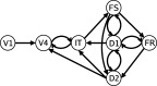
A large‐scale neural computational network is a simple, yet neurobiologically realistic model of a brain circuit that is able to simulate data at multiple spatial and temporal levels. We here employ one such model that was developed by Tagamets and Horwitz [Horwitz and Tagamets, 1999; Tagamets and Horwitz, 1998] to simulate region‐specific fMRI data (see Fig. 1). This model has previously been used to investigate functional and effective connectivity [Horwitz et al., 2005; Kim and Horwitz, 2008; Lee et al., 2006]. This network performs a visual delayed match‐to‐sample (DMS) task for two‐dimensional object shapes. The model contains four major brain regions; the primary visual cortex (V1/V2), secondary visual cortex (V4), inferior temporal cortex (IT), and prefrontal cortex (PFC). The PFC consists of four sub‐populations of units named FS (stimulus‐sensitive units), D1 (units active during the delay between stimuli), D2 (units active during stimulus presentation and during the delay), and FR (units whose activity increases if there is a match between the first and second stimuli of a DMS trial). Although the PFC units are likely to be located in the same brain area, we will treat these four sub‐modules as if they correspond to spatially separated brain regions because the anatomical connections among these four sub‐modules are complex and can provide some interesting challenges for connectivity analysis. Every module or sub‐module is thus composed of multiple basic units, each representing a simplified cortical column; the basic unit comprises an interacting pair of excitatory‐inhibitory neurons (modified Wilson‐Cowan units [Wilson and Cowan, 1972]). Regions are linked by both feed‐forward and feedback connections. The simulated electrophysiological activity in each module has been shown to be similar to data found in primate studies (see Tagamets and Horwitz [1998] for details).
Figure 1.

Structural (anatomic) large‐scale neural model used to simulate the fMRI data. See text and Tagamets and Horwitz [1998] for details and definitions. [Color figure can be viewed in the online issue, which is available at www.interscience.wiley.com.]
For the present work, an fMRI study is simulated by presenting stimuli to an area of the model that represents the lateral geniculate nucleus. The fMRI response is simulated by temporally and spatially integrating the absolute value of the synaptic activity in each region over an appropriate time course, and for simulating fMRI, convolving these values with a function representing hemodynamic delay, and downsampling the resulting time series at time intervals corresponding to the TR used [Horwitz and Tagamets, 1999]. It is on these data that we perform analysis of effective connectivity.
Structural Equation Modeling
SEM is a common statistical approach for addressing effective connectivity that has been successfully adopted to functional brain imaging data [Büchel and Friston, 1997; Kim et al., 2007; McIntosh and Gonzalez‐Lima, 1994; McIntosh et al., 1994]. In the present study, the structural (i.e., anatomical) model is defined as given by the large‐scale visual model shown in Figure 1 and reproduced in Figure 2 in terms of a structural model. A Goodness‐of‐Fit index (GFI) is evaluated to test the goodness‐of‐fit of the functional model, which indicates the effective connectivity of each anatomical connection of the structural model. A GFI higher than 0.85 indicates an adequate fit of the network model [Schlösser et al., 2003, 2006]. The effective connectivity parameters are estimated by minimizing the discrepancy between the correlation matrix from simulated fMRI data and the correlation matrix implied by the functional model. An estimated effective connectivity coefficient represents the change in activity of one region from a unit change in activity of another region [Bollen, 1989].
Figure 2.
Structural model used for SEM analysis.
Partial Correlation Analysis
Partial correlation analysis for effective connectivity investigation relies on inferring the partial correlation matrix Π, given the BOLD fMRI data [Marrelec et al., 2006b]. When specifically considering the interactions between two regions within a set of N regions, partial correlation removes that part of the statistical variations in the signals of these two regions that can be accounted for by the variations of the other N − 2 regions [Whittaker, 1990]. For this reason, partial correlation has been hypothesized to be more closely related to effective connectivity than is the classical, i.e., marginal, correlation [Marrelec et al., 2005a]. Estimation of the partial correlation matrix is based on a Bayesian sampling scheme that approximates the posterior distribution of the partial correlation matrix given the data, p(Π|y) [Marrelec et al., 2005b].
The Bayesian inference procedure allows one to access not only an estimate of the partial correlation matrix (which, for large datasets, is usually close to the sample partial correlation matrix that can be evaluated directly from the data), but also standard deviations, significance values, and, more generally, any statistical quantity of interest. For more details, the interested reader is referred to Marrelec et al. [2005b, 2007].
SYNTHETIC DATA
LSM Data Generation
The region‐specific neural activity was generated by the large‐scale neural model during performance of the visual DMS task. The task design consisted of 10 blocks of trials, each block comprising 6 DMS trials and 6 “passive‐viewing” (PV) trials, corresponding to the control condition in which passively‐viewed scrambled visual objects were presented. Each trial consisted of the presentation of the first stimulus for 1 s, a delay of 1.5 s, the display of the second stimulus for 1 s, and then 1 s for the response period (which includes the inter‐trial interval).
Note that half of the regional neuronal population was assigned as non‐specific neurons, to which noise patterns are presented asynchronously and randomly relative to the presentation of the stimuli. Specific and non‐specific neurons have their synaptic connections modified in a random way on each trial (see Horwitz et al. [2005] for details). This effect provided the trial‐to‐trial variability that allows us to model the interactions between the neuronal network elements responding to the task of interest.
The block‐to‐block variability was expressed using different values of the attention parameter that informs the model about which task (DMS or PV) to perform. This parameter modulates how D2 delay units respond to a given stimulus; e.g., the higher the attention, the better the representation that is maintained during the delay period. The attention values for the DMS task ranged from 0.22 to 0.31 (arbitrary units) in steps of 0.01 for each block. The attention parameter for all PV task trials was fixed to 0.05.
The subject‐to‐subject variability could be instantiated by varying the different anatomical interregional connection weights between subjects (see Horwitz et al. [2005] for details), hence allowing us to generate data corresponding to a group of subjects. However, in this study, to compare the partial correlation and estimated effective connectivity parameters, we only used one simulated subject and thus employed only one set of anatomical connection weights. The simulated synaptic activities (or synthetic neural signals) were integrated over each region and convolved with a gamma function representing the hemodynamic delay [Boynton et al., 1996] to produce a temporally smoothed BOLD time‐series. We then down‐sampled it every 2 s (TR = 2 s) to produce the simulated fMRI time‐series. Each regional fMRI time series was separated into the DMS or PV task components, and each one was normalized to a zero mean and unit variance.
SEM Analysis
The simulated fMRI dataset for each condition (DMS or PV) was fitted to the structural model shown in Figure 2, which corresponds exactly to the one used to simulate the data. The model's goodness of fit index demonstrated a good fit (GFI = 0.96 for task, and GFI = 0.93 for control condition). The effective connectivity parameters were estimated by minimizing the maximum‐likelihood function,
where k is a number of variables (or brain regions), S is the sample correlation matrix, and Σ(θ) is the implied correlation matrix given a vector of free effective connectivity parameters θ. All models were obtained using maximum likelihood methods implemented in LISREL software (version 8) [Joreskog and Sorborn, 1996]. Each effective connectivity parameter estimate divided by its standard error produced a t‐value, whose significance was determined at a 95% confidence level (see Tables I and II as well as Figure 3 for details).
Table I.
SEM analysis
| V1 | V4 | IT | FS | D1 | D2 | FR | v | |
|---|---|---|---|---|---|---|---|---|
| V1 | 0.75 | 0.59 | 0.46 | 0.16 | 0.09 | 0.31 | 1 | |
| V4 | 0.72 | 0.93 | 0.83 | 0.49 | 0.42 | 0.66 | 0.13 | |
| IT | 0.60 | 0.95 | 0.95 | 0.64 | 0.57 | 0.76 | 0.1 | |
| FS | 0.55 | 0.92 | 0.98 | 0.65 | 0.63 | 0.78 | 0.1 | |
| D1 | 0.15 | 0.56 | 0.62 | 0.64 | 0.82 | 0.67 | 0.34 | |
| D2 | 0.12 | 0.58 | 0.65 | 0.67 | 0.91 | 0.56 | 0.37 | |
| FR | 0.24 | 0.69 | 0.77 | 0.79 | 0.88 | 0.84 | 0.36 | |
| v | 1 | 0.11 | 0.09 | 0.03 | 0.18 | 0.24 | 0.14 |
Observed correlations from simulated fMRI data and estimated error variances (v) during the DMS task (lower triangular matrix) and the control condition (upper triangular matrix).
Table II.
SEM results
| Task condition (DMS) | Control condition (PV) | |||||
|---|---|---|---|---|---|---|
| Eff. conn. | S. E. | t‐value (P) | Eff. conn. | S. E. | t‐value (P) | |
| V1→V4 | 0.48 | 0.04 | 13.8 (<0.001) | 0.49 | 0.04 | 13.4 (<0.001) |
| V4→IT | 0.8 | 0.03 | 25.6 (<0.001) | 0.75 | 0.03 | 23.6 (<0.001) |
| IT→V4 | 0.35 | 0.04 | 8.18 (<0.001) | 0.43 | 0.04 | 9.84 (<0.001) |
| IT→FS | 0.96 | 0.02 | 54.6 (<0.001) | 0.92 | 0.03 | 27.5 (<0.001) |
| FS→D1 | 0.03 | 0.08 | 0.35 (0.73) | 0.12 | 0.22 | 0.56 (0.58) |
| FS→D2 | 0.03 | 0.1 | 0.27 (0.79) | 0.23 | 0.15 | 1.58 (0.12) |
| FS→FR | 0.39 | 0.04 | 9.5 (<0.001) | 0.65 | 0.11 | 5.68 (<0.001) |
| D1→IT | 0.02 | 0.07 | 0.25 (0.8) | 0.12 | 0.05 | 2.32 (<0.001) |
| D1→FS | 0.03 | 0.02 | 1.65 (0.1) | 0.02 | 0.04 | 0.48 (0.63) |
| D1→D2 | 0.43 | 0.11 | 3.99 (<0.001) | 0.48 | 0.1 | 4.78 (<0.001) |
| D1→FR | 0.56 | 0.07 | 8.48 (<0.001) | 0.17 | 0.26 | 0.67 (0.5) |
| D2→V4 | 0.27 | 0.04 | 6.24 (<0.001) | 0.08 | 0.04 | 1.76 (0.08) |
| D2→IT | 0.13 | 0.07 | 1.88 (0.06) | 0.1 | 0.05 | 1.96 (0.05) |
| D2→D1 | 0.57 | 0.11 | 5.22 (<0.001) | 0.39 | 0.11 | 3.41 (<0.001) |
| FR→D1 | 0.16 | 0.13 | 1.23 (0.22) | 0.18 | 0.31 | 0.58 (0.56) |
| FR→D2 | 0.2 | 0.15 | 1.39 (0.17) | −0.09 | 0.15 | −0.59 (0.56) |
The estimated effective connectivity parameters with standard errors, and their t‐values (P‐values). Effective connectivity parameters were estimated by an iteration procedure minimizing the maximum likelihood function used in LISREL software. Bold indicates the links that were significantly different from zero at P < 0.05.
Figure 3.

Effective connectivity diagram for each condition. Solid arrows indicate effective connections that are significantly different from zero at P < 0.05. Dashed arrows are not statistically significant.
The results of the SEM analysis revealed that most of the structural links modeled by SEM had significant effective connections, in both the DMS and the PV conditions. One difference between the two conditions was particularly interesting: whereas the effective connection between D1 and FR did not significantly differ from zero in the control condition, it became significant in the DMS condition. This result is a rather good reflection of the underlying neural relationships. In the model, a positive match between the two stimuli in the DMS occurs when there is simultaneously strong neural activity in D1 and FS, whose neurons in turn project to the response selective neurons in FR. During PV, the attention level is set at a low value, which results in reduced activity in D1. As a result, the neurons in FR never receive enough input activity to cause them to be activated.
Interestingly, five connections of the large‐scale neural model (bidirectional FS–D1, D1→IT, FR→D1, and FR→D2) projecting from excitatory neurons in one area to inhibitory interneurons in another were expected to be associated with negative values of effective connectivity in the structural model. These connections were found to be nonsignificant (except for D1→IT in the control condition). The reason is that the dynamics of the units are such that activation of the inhibitory units tends to reduce a module's activity resulting in the module having low activity that becomes uncorrelated from the input module. For a significant fMRI effective connection, the neural activity along the structural link needs to be more sustained than transient.
The results of the SEM analysis of the simulated fMRI data, in conclusion, show that most of the excitatory anatomical links in the model have significant effective connectivity during the DMS task condition, thus reflecting the underlying neural relationships.
Partial Correlation Analysis
We sampled L = 10,000 matrices  from the posterior distribution of the partial correlation matrix. From this sample, we approximated all statistical quantities of interest (such as mean, variance, significance level). We summarized the estimated values for both the partial and marginal correlation coefficients in Tables III and IV and also plotted these estimates in Figure 4.
Table III.
Estimated marginal and partial correlation matrices corresponding to the DMS task condition
| V1 | V4 | IT | FS | D1 | D2 | FR | |
|---|---|---|---|---|---|---|---|
| V1 | — | 0.72 ± 0.04 (<10−4) | 0.60 ± 0.05 (<10−4) | 0.55 ± 0.06 (<10−4) | 0.15 ± 0.08 (0.026) | 0.12 ± 0.08 (0.14) | 0.24 ± 0.08 (10−4) |
| V4 | 0.59 ± 0.05 (<10−4) | — | 0.95 ± 0.01 (<10−4) | 0.93 ± 0.01 (<10−4) | 0.56 ± 0.06 (<10−4) | 0.58 ± 0.05 (<10−4) | 0.69 ± 0.04 (<10−4) |
| IT | −0.01 ± 0.08 (0.47) | 0.48 ± 0.06 (<10−4) | — | 0.98 ± 0.003 (<10−4) | 0.62 ± 0.05 (<10−4) | 0.65 ± 0.05 (<10−4) | 0.77 ± 0.04 (<10−4) |
| FS | −0.10 ± 0.08 (0.11) | −0.04 ± 0.08 (0.30) | 0.83 ± 0.02 (<10−4) | — | 0.63 ± 0.05 (<10−4) | 0.67 ± 0.05 (<10−4) | 0.78 ± 0.03 (<10−4) |
| D1 | 0.17 ± 0.08 (0.017) | −0.04 ± 0.08 (0.30) | −0.01 ± 0.08 (0.47) | −0.09 ± 0.08 (0.12) | — | 0.91 ± 0.01 (<10−4) | 0.88 ± 0.02 (<10−4) |
| D2 | −0.30 ± 0.08 (10−4) | 0.14 ± 0.08 (0.034) | −0.04 ± 0.08 (0.33) | 0.09 ± 0.08 (0.13) | 0.68 ± 0.04 (<10−4) | — | 0.84 ± 0.02 (<10−4) |
| FR | −0.20 ± 0.08 (7 × 10⁻³) | 0.00 ± 0.08 (0.48) | 0.08 ± 0.08 (0.15) | 0.13 ± 0.08 (0.046) | 0.57 ± 0.05 (<10−4) | −0.01 ± 0.08 (0.42) | — |
Upper triangular matrix: marginal correlation; lower triangular matrix: partial correlation. For each pair, the mean ± standard deviation are reported, as well as the significance. Significant correlations (P < 10−4) are represented in bold.
Table IV.
Estimated marginal and partial correlation matrices corresponding to the control (passive viewing) condition
| V1 | V4 | IT | FS | D1 | D2 | FR | |
|---|---|---|---|---|---|---|---|
| V1 | — | 0.75 ± 0.04 (<10−4) | 0.59 ± 0.05 (<10−4) | 0.46 ± 0.06 (<10−4) | 0.16 ± 0.08 (0.026) | 0.09 ± 0.08 (0.14) | 0.31 ± 0.07 (10−4) |
| V4 | 0.56 ± 0.05 (<10−4) | — | 0.93 ± 0.01 (<10−4) | 0.83 ± 0.03 (<10−4) | 0.49 ± 0.06 (<10−4) | 0.42 ± 0.07 (<10−4) | 0.66 ± 0.05 (<10−4) |
| IT | −0.03 ± 0.08 (0.36) | 0.67 ± 0.04 (<10−4) | — | 0.95 ± 0.01 (<10−4) | 0.64 ± 0.05 (<10−4) | 0.57 ± 0.06 (<10−4) | 0.76 ± 0.04 (<10−4) |
| FS | −0.12 ± 0.08 (0.067) | −0.21 ± 0.08 (3.1 × 10⁻³) | 0.75 ± 0.03 (<10−4) | — | 0.65 ± 0.05 (<10−4) | 0.63 ± 0.05 (<10−4) | 0.78 ± 0.03 (<10−4) |
| D1 | −0.05 ± 0.08 (0.28) | −0.11 ± 0.08 (0.09) | 0.25 ± 0.07 (4 × 10⁻⁴) | −0.22 ± 0.07 (1.8 × 10⁻³) | — | 0.81 ± 0.03 (<10−4) | 0.66 ± 0.05 (<10−4) |
| D2 | −0.08 ± 0.08 (0.17) | −0.02 ± 0.08 (0.39) | −0.08 ± 0.08 (0.15) | 0.27 ± 0.07 (5 × 10⁻⁴) | 0.67 ± 0.04 (<10−4) | — | 0.55 ± 0.06 (<10−4) |
| FR | −0.13 ± 0.08 (0.048) | 0.12 ± 0.08 (0.075) | −0.02 ± 0.08 (0.40) | 0.25 ± 0.08 (8·× 10−4) | 0.32 ± 0.07 (<10−4) | −0.13 ± 0.08 (0.047) | — |
Upper triangular matrix: marginal correlation; lower triangular matrix: partial correlation. For each pair the mean ± standard deviation are reported, as well as the significance. Significant correlations (P < 10−4) are represented in bold.
Figure 4.
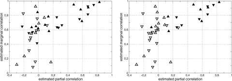
Two‐dimensional representation of the links indexed by their estimated partial (x‐axis) and marginal (y‐axis) correlation coefficients. Full symbols relate to links that are taken into account in the large‐scale neural (LSN) model (left) or computed as significant by SEM analysis (right), while empty symbols relate to links that are absent in the same model. Up arrows stand for links during the task condition, Down arrows for links during the task condition.
To determine whether each link should be considered as functionally relevant or not and classify each pair of regions accordingly, two methods were implemented. The first, more traditional, method [Marrelec et al., 2006b, 2007] simultaneously relied on a simple thresholding of the marginal correlation matrix to a very high level (P < 10−4) and of the partial correlation matrix to somewhat lower levels (values used were: P < 0.05, P < 0.01, P < 10−3, and P < 10−4). The second method takes advantage of the seemingly different relationships between partial and marginal correlations for relevant and irrelevant links, respectively, that can be observed in Figure 4. To separate both groups of links using only information relative to partial and marginal correlation, we considered all links in the two dimensional partial/marginal correlation plane and classified them into two sets using a two‐dimensional mixture of Gaussian models procedure. This procedure provided each link (represented as a point in the two dimensional partial/marginal plane) with a probability that it belongs to either of the two classes. The class containing links characterized by high partial correlation values is then selected as the set of relevant links, the other being the class of irrelevant links. In Figure 5, we represented the probability that each link belongs to the functionally relevant class. Graph structures obtained by both the thresholding and the classification approaches are represented in Figure 6.
Figure 5.
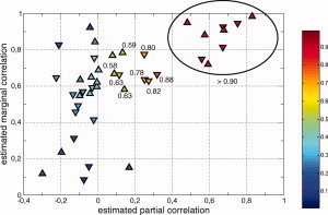
Correlation classification. Each link is indexed by its estimated partial (x‐axis) and marginal (y‐axis) correlation. Up and down arrows relate to links that correspond to the task and control conditions, respectively. The color codes the probability P for a given link to be included in the set of relevant links. The probability values have been added for links with P > 0.5. We used an ellipse to gather all links with a probability larger than 0.9.
Figure 6.
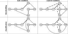
Significant effective connections, obtained from either the thresholding (top) or the classification (bottom) method. For the thresholding method, we only selected connections with significant marginal and partial correlation coefficients. Significance was set at 10−4 for marginal correlation, while it was varied from 0.05 to 10−4 for partial correlation. Links that pass all tests are represented by solid lines. Links that appear at the 0.001, 0.01, or 0.05 thresholds are represented by broken lines, broken‐dotted lines, and dotted lines, respectively. For the classification method, links that have a probability higher than 0.9 of belonging to the set of relevant connections are represented by solid lines; between 0.8 and 0.9 by broken lines; between 0.7 and 0.8 by broken‐dotted lines; between 0.5 and 0.7 by dotted lines.
Comparison of SEM and Partial Correlation
Visual comparison of the results from the two methods as represented by the solid lines in Figures 3 (SEM results) and 6 (the partial correlation results) shows remarkable agreement (see Table V for a summary). For both the task and the control conditions, all connections considered as significant by SEM were successfully retrieved with partial correlation and either the thresholding or the classification method, even if sometimes at a rather low threshold (see, e.g., FS–FR and V4–D2 for the task condition; FS–FR for the control condition). Regarding links that were not significant with SEM, however, some were similarly classified as irrelevant by partial correlation (e.g., V1–IT), while others were considered as potentially relevant (FS–D2 for the task condition; V4–FS, V4–FR, FS–D1, and FS–D2 for the control condition). The thresholding and the classification methods may furthermore disagree regarding the relevance of such links (see, e.g., FS–D2 in the task condition or FS–D1 in the control condition). Among these links, some are links that were taken into account in the LSN model (FS–D2 for the task condition; FS–D1 and FS–D2 for the control condition), while others were not (V4–FS and V4–FR for the control condition).
Table V.
Comparison of results from SEM analysis and partial correlation analysis with the true LSN model
| ∈ LSN | ∉ LSN | |||
|---|---|---|---|---|
| ∈ SEM | ∉ SEM | ∈ SEM | ∉ SEM | |
| ∈ PC | 7/6 | 1/4 | — | 0/2 |
| ∉ PC | 0/0 | 4/2 | — | 9/7 |
Links are classified according to three criteria: whether they are present in the LSN model (∈ LSN) or not (∉ LSN); whether they are detected as significant by the SEM analysis (∈ SEM) or not (∉ SEM), and whether they are detected as being relevant by the partial correlation analysis (∈ PC) or not (∉ PC), with either the thresholding (P < 0.05) or the classification (P > 0.5) method. For each class, we report the number of links for both the task and the control conditions. For instance, there are seven links modeled in the LSN model that were detected by both SEM and partial correlation in the task condition and six in the control condition.
DISCUSSION AND PERSPECTIVES
In this study, we provide a first validation of partial correlation analysis compared with the classical SEM approach using large‐scale simulated data.
As has been long noted [e.g., McIntosh et al., 1994], marginal correlation alone is not a good predictor of the presence or absence of a link (i.e., effective connection). Indeed, in our case, (relatively) low marginal correlations were associated with functional links that were present in the SEM analysis (e.g., D2–V4 in the control condition), while higher marginal correlations were observed between pairs of regions that were not connected with one another (e.g., V4–FS). In this example, one can clearly see the chain effect induced by marginal correlation when considering connections from V1 to other regions: even though V1 is connected only to V4, the marginal correlation between V1 and other region decreases but remains significant when one moves from V4 to IT to frontal regions. This property makes marginal correlation redundant as the set of relevant links is very likely to be a subset of the significant marginal correlation coefficients.
Another cogent illustration that marginal correlation is less able to predict a link than partial correlation is given by the SEM analysis itself. Compared with the true underlying structural model, SEM analysis did not identify all of the anatomical connections as functionally significant. Most connections that were left aside by this kind of analysis were not those with low marginal correlation values, but rather those with the lowest partial correlation coefficients. All in all, marginal correlation appears as a useful tool in the rare situations where it is nonsignificant, in which cases the corresponding link can probably not be trusted (e.g., V1 with D1, D2 and FR in both conditions).
There are mainly two reasons why we reported estimates of marginal correlation in this work instead of simply ignoring them as being completely irrelevant. The first is that theoretical considerations have led us to posit that marginal correlation is not a good measure of direct interaction [Marrelec et al., 2005a]. Previous results have tended to confirm this hypothesis, but, so far, there have been insufficient grounds to completely discard marginal correlation. Second, marginal correlation has proven a valuable measure of functional connectivity in previous studies [Bellec et al., 2006; Biswal et al., 1995, 1997; Bokde et al., 2001]. We were consequently driven to believe that this quantity carried some information regarding the interaction pattern.
In contrast, the information carried by partial correlation is both more relevant for functional interaction analysis and more complex. Almost all large values of partial correlations were rightfully detected as belonging to the class of relevant links regardless of the method and threshold used. Large values included the V1–V4–IT–FS stream. The significance of partial correlation is related to the skeleton of the connectivity structure much more closely than marginal correlation could be. However, depending on the threshold, the set of significant partial correlations is sometimes larger, sometimes smaller, than the set of existing links; hence the importance of selecting a proper threshold. To determine which of the partial correlations should be used to infer a link in the model, one should look at different levels of threshold, for different conditions, and also possibly compare the results with prior information. A few connections modeled in the LSN were never found, such as FS–D1 for the task condition. However, all these connections also had insignificant effective connections in the SEM analysis, and many represented, at the neural level, inhibitory connections whose transient pattern of activity, as mentioned above, tends to reduce a module's activity resulting in the module now having low activity that becomes uncorrelated from the input module. In this case, both SEM and partial correlation analysis of fMRI data agreed, but both show that fMRI can be limited in exhibiting all relevant patterns of interactions that are instantiated by the connections between regions.
From this study, it clearly emerges that relevant information regarding brain functional interactions is carried by both partial and marginal correlation. Both methods to select potential connections (i.e., threshold and classification) take advantage of both types of correlations to perform optimal inference. Although the thresholding method is rather classical, the classification/outlier detection method might prove more effective if the structure of correlation observed in this particular case of synthetic datasets turns out to be more general, i.e., also valid for real data. The upside of classification is that the procedure yields a result that can be interpreted as the probability that a given link belongs to the class of “existing,” as opposed to “nonexisting,” links. As such, it is more meaningful than a P‐value. To prove this point and be able to validate the use of this approach for link selection, future studies must move from simulated data to real data. Even with partial correlation, the discrimination between links that are present and links that are absent is a complex task. Thresholding and classification provide results that are mostly consistent, but with some differences.
All values of marginal correlation calculated and observed were positive. By contrast, some partial correlation coefficients were found to be (significantly) lower than zero. The meaning, i.e., the interpretation and relevance, of such values remain unclear. Present connections within the large scale model generated mostly positive values, with the exception of IT–D1, IT–D2, FS–D1, and D2–FR for the task condition and V4–D2, IT–D2, FS–D1, D2–FR for the control condition. Among these, only FS–D1 (P = 1.8 × 10⁻³) and D2–FR (P = 0.047) for the control condition had a significant value. None of these values corresponded to a significant effective connection.
For an efficient use of partial correlation as a measure of effective connectivity in fMRI, we still have to solve the issue of determining how a functional interaction is defined. In SEM, an interaction is obviously defined by the presence of an arrow. With partial correlation analysis, all that can be done is declare a connection present or absent in terms of some threshold criterion on the correlation coefficient or its associated P‐value. The issue of change between conditions should also be considered, since SEM is often used not so much as a way to examine the true effective connectivity underlying a given task as a way to analyze how certain interactions are influenced by a change in task.
The results detailed in this article are based on the comparison of SEM and partial correlation analyses with the true connectivity structure used to generate the synthetic data. The model constitutes a realistic large scale neural model [Tagamets and Horwitz, 1998] that has been constructed with care so that it can emulate observed features of the cerebral cortex, such as neuronal activity and BOLD signal in multiple, interconnected brain regions [Horwitz, 2005]. Also, this model has been used to test certain aspects of functional and effective connectivity [Horwitz et al., 2005; Lee et al., 2006]. In what way this model really generates realistic data in terms of interactions needs to be further investigated. For instance, it is not obvious that the plot of partial and marginal correlation coefficients calculated from real data will generate the same shape as was observed in Figures 4 and 5. As a corollary, the thresholding methods proposed here also have to be validated and, possibly, adapted to real data.
The exact relationship between partial correlation and structural model analyses remains to be elucidated. Although each structural model in the form of a directed acyclic graph entails specific patterns of correlation [Lauritzen, 1996; Marrelec et al., 2005a, b; Pearl, 2001; Whittaker, 1990], not all patterns of marginal and/or partial correlation can unambiguously be associated with a structural model [Pearl and Wermuth, 1994]. Regarding parameter estimation, while directed acyclic graphs must abide by constraints of sparcity to allow for correct estimation of the path coefficients, no such constraint exists for partial correlation analysis, which could potentially identify any connection amongst the graph nodes. The properties of cyclic graphs, which are commonly used in effective connectivity, are much less well known and so is their relation with correlation. Although it is uncertain whether and how we could take advantage of differential properties of partial correlation (particularly since it has only been shown to make sense within a more global analysis framework involving SEM), this study showed that partial correlation usually extracts functional connections that are relevant for SEM analysis.
As detailed in Penny et al. [2004], it can be shown that SEM is a simplified version of DCM. While SEM is an accepted tool to investigate effective connectivity in fMRI data analysis of continuous or block‐designed experiments [see, e.g., Büchel and Friston, 1997; Gonçalves et al., 2001; McIntosh and Gonzalez‐Lima, 1994; Penny et al., 2004], DCM is arguably more general in its underlying model, its inference framework, and the variety of data that it can possibly analyze (e.g., event‐related). Since a recent study has demonstrated the relation between the LSN model and DCM [Lee et al., 2006], it would be of interest to examine in what measure partial correlation analysis provides results that are consistent with DCM and whether the former could provide insightful hypotheses regarding what model or class of models could be proposed for DCM analysis. For the purpose of our investigation, use of SEM was justified by the fact that, unlike DCM, the statistical model underlying SEM is quite simple, has been investigated in depth from a theoretical perspective, and is strongly related to that underlying marginal and partial correlation. As such, we hope it also makes it possible to reach a better understanding of functional connectivity.
In summary, we have shown, using a neurobiologically realistic network model to generate simulated fMRI data, that partial correlation analysis produces a good estimate of which anatomical nodes should be linked together for effective connectivity analysis using SEM. We believe the results obtained provide rather compelling evidence that a mostly data‐driven investigation of effective connectivity is possible.
INFERRING MARGINAL AND PARTIAL CORRELATIONS
Using standard Bayesian theory, assuming a classical Jeffreys' prior for the N‐by‐N covariance matrix Σ, and T independent and identically distributed (i.i.d.) Gaussian samples, the posterior probability of Σ, given the data y, p(Π|y), has an inverse Wishart distribution with T − 1 degrees of freedom and scale matrix S that is proportional to the sample covariance matrix,
where  is the temporal average. We then resort to a sampling scheme. For sample l,
sample Σ[l] according to its inverse Wishart distribution [Gelman et al., 1998, Appendix A].
calculate
 from
from  [Whittaker, 1990].
Once a large number L has been sampled according to this procedure, any statistic can be approximated by its sample counterpart. For instance,
REFERENCES
- Achard S,Salvador R,Whitcher B,Suckling J,Bullmore E (2006): A resilient, low‐frequency, small world human brain functional network with highly connected association cortical hubs. J Neurosci 26: 63–72. [DOI] [PMC free article] [PubMed] [Google Scholar]
- Beckmann CF,DeLuca M,Devlin JT,Smith SM (2005): Investigations into resting‐state connectivity using independent component analysis. Philos Trans R Soc Lond B Biol Sci 360: 1001–1013. [DOI] [PMC free article] [PubMed] [Google Scholar]
- Bellec P,Perlbarg V,Jbabdi S,Pélégrini‐Issac M,Anton JL,Doyon J,Benali H (2006): Identification of large‐scale networks in the brain using fMRI. Neuroimage 29: 1231–1243. [DOI] [PubMed] [Google Scholar]
- Biswal B,Yetkin FZ,Haughton VM,Hyde JS (1995): Functional connectivity in the motor cortex of resting human brain using echoplanar MRI. Magn Reson Med 34: 537–541. [DOI] [PubMed] [Google Scholar]
- Biswal BB,Kylen JV,Hyde JS (1997): Simultaneous assessment of flow and BOLD signals in resting‐state functional connectivity maps. NMR Biomed 10: 165–170. [DOI] [PubMed] [Google Scholar]
- Bokde AL,Tagamets MA,Friedman RB,Horwitz B (2001): Functional interactions of the inferior frontal cortex during the processing of words and word‐like stimuli. Neuron 30: 609–617. [DOI] [PubMed] [Google Scholar]
- Bollen KA (1989): Structural Equation with Latent Variables. New York: Wiley‐interscience. [Google Scholar]
- Boynton GM,Engel SA,Glover GH,Heeger DJ (1996): Linear systems analysis of functional magnetic resonance imaging in human V1. J Neurosci 16: 4207–4221. [DOI] [PMC free article] [PubMed] [Google Scholar]
- Bressler SL,Tognoli E (2006): Operational principles of neurocognitive networks. Int J Psychophysiol 60: 139–148. [DOI] [PubMed] [Google Scholar]
- Büchel C,Friston KJ (1997): Modulation of connectivity in visual pathways by attention: Cortical interactions evaluated with structural equation modelling and fMRI. Cereb Cortex 7: 768–778. [DOI] [PubMed] [Google Scholar]
- Damoiseaux JS,Rombouts SA,Barkhof F,Scheutens P,Stam CJ,Smith SM,Beckmann CF (2006): Consistent resting‐state networks across healthy subjects. Proc Natl Acad Sci USA 103: 13848–13853. [DOI] [PMC free article] [PubMed] [Google Scholar]
- Dodel S,Golestani N,Pallier C,ElKouby V,Le Bihan D,Poline JB (2005): Condition‐dependent functional connectivity: Syntax network in bilinguals. Philos Trans R Soc Lond B Biol Sci 360: 921–935. [DOI] [PMC free article] [PubMed] [Google Scholar]
- Esposito F,Formisano E,Seifritz E,Goebel R,Morrone R,Tedeschi G,Salle FD (2002): Spatial independent component analysis of functional MRI time‐series: To what extent do results depend on the algorithm used? Hum Brain Mapp 16: 146–157. [DOI] [PMC free article] [PubMed] [Google Scholar]
- Esposito F,Scarabino T,Hyvarinen A,Himberg J,Formisano E,Comari S,Tedeschi G,Goebel R,Seifritz E,Di Salle F (2005): Independent component analysis of fMRI group studies by self‐organizing clustering. Neuroimage 25: 193–205. [DOI] [PubMed] [Google Scholar]
- Friston KJ (1994): Functional and effective connectivity in neuroimaging: A synthesis. Hum Brain Mapp 2: 56–78. [Google Scholar]
- Friston KJ,Harrison L,Penny W (2003): Dynamic causal modelling. Neuroimage 19: 1273–1302. [DOI] [PubMed] [Google Scholar]
- Gelman A,Carlin JB,Stern HS,Rubin DB (1998): Bayesian Data Analysis. Texts in Statistical Science. London: Chapman & Hall. [Google Scholar]
- Gonçalves MS,Hall DA,Johnsrude IS,Haggard MP (2001): Can meaningful effective connectivities be obtained between auditory cortical regions? Neuroimage 14: 1353–1360. [DOI] [PubMed] [Google Scholar]
- Greicius MD,Menon V (2004): Default‐mode activity during a passive sensory task: Uncoupled from deactivation but impacting activation. J Cogn Neurosci 16: 1484–1492. [DOI] [PubMed] [Google Scholar]
- Greicius MD,Krasnow B,Reiss AL,Menon V (2003): Functional connectivity in the resting brain: A network analysis of the default mode hypothesis. Proc Natl Acad Sci USA 100: 253–258. [DOI] [PMC free article] [PubMed] [Google Scholar]
- Himberg J,Hyvärinen A,Esposito F (2004): Validating the independent components of neuroimaging time series via clustering and visualization. Neuroimage 22: 1214–1222. [DOI] [PubMed] [Google Scholar]
- Horwitz B (2003): The elusive concept of brain connectivity. Neuroimage 19: 466–470. [DOI] [PubMed] [Google Scholar]
- Horwitz B (2004): Relating fMRI and PET signals to neural activity by means of large‐scale neural models. Neuroinformatics 2: 251–266. [DOI] [PubMed] [Google Scholar]
- Horwitz B (2005): Integrating neuroscientific data across spatiotemporal scales. C R Biol 328: 109–118. [DOI] [PubMed] [Google Scholar]
- Horwitz B,Tagamets MA (1999): Predicting human functional maps with neural net modeling. Hum Brain Mapp 8: 137–142. [DOI] [PMC free article] [PubMed] [Google Scholar]
- Horwitz B,Tagamets MA,McIntosh AR (1999): Neural modeling, functional brain imaging and cognition. Trends Cogn Sci 3: 91–98. [DOI] [PubMed] [Google Scholar]
- Horwitz B,Warner B,Fitzer J,Tagamets MA,Husain FT,Long TW (2005): Investigating the neural basis for functional and effective connectivity. Application to fMRI. Philos Trans R Soc Lond 360: 1093–1108. [DOI] [PMC free article] [PubMed] [Google Scholar]
- Huettel SA,Song AW,McCarthy G (2004): Functional Magnetic Resonance Imaging. Sunderland: Sinauer. [Google Scholar]
- Joreskog KG,Sorborn D (1996): LISREL 8 User's Reference Guide. Chicago: Scientific Sofware International. [Google Scholar]
- Kim J,Horwitz B (2008): Investigating the neural basis for fMRI‐based functional connectivity in a blocked design: Application to interregional correlations and psycho‐physiological interactions. Magn Reson Imaging, doi:10.1016/j.mri.2007.10.011. [DOI] [PubMed] [Google Scholar]
- Kim J,Zhu W,Chang L,Bentler PM,Ernest T (2007): Unified structural equation modeling approach for the analysis of multisubject, multivariate functional MRI data. Hum Brain Mapp 28: 85–93. [DOI] [PMC free article] [PubMed] [Google Scholar]
- Lauritzen SL (1996): Graphical Models. Oxford: Oxford University Press. [Google Scholar]
- Lee L,Friston K,Horwitz B (2006): Large‐scale neural models and dynamic causal modelling. Neuroimage 30: 1243–1254. [DOI] [PubMed] [Google Scholar]
- Lee L,Harrison LM,Mechelli A (2003): A report of the functional connectivity workshop, Düsseldorf 2002. Neuroimage 19: 457–465. [DOI] [PubMed] [Google Scholar]
- Marrelec G,Daunizeau J,Pélégrini‐Issac M,Doyon J,Benali H (2005a): Conditional correlation as a measure of mediated interactivity in fMRI and MEG/EEG. IEEE Trans Signal Process 53: 3503–3516. [Google Scholar]
- Marrelec G,Doyon J,Pélégrini‐Issac M,Benali H (2005b): Heading for data‐driven measures of effective connectivity in functional MRI. In: Proceedings of the International Joint Conference on Neural Networks. pp 1528–1533.
- Marrelec G,Bellec P,Benali H (2006a): Exploring large‐scale brain networks. J Physiol Paris 100: 171–181. [DOI] [PubMed] [Google Scholar]
- Marrelec G,Krainik A,Duffau H,Pélégrini‐Issac M,Lehéricy S,Doyon J,Benali H (2006b): Partial correlation for functional brain interactivity investigation in functional MRI. Neuroimage 32: 228–237. [DOI] [PubMed] [Google Scholar]
- Marrelec G,Horwitz B,Kim J,Pélégrini‐Issac M,Benali H,Doyon J (2007): Using partial correlation to enhance structural equation modeling of functional MRI data. Magn Reson Imaging 25: 1181–1189. [DOI] [PubMed] [Google Scholar]
- McIntosh AR,Gonzalez‐Lima F (1994): Structural equation modeling and its aplication to network analysis of functional brain imaging. Hum Brain Mapp 2: 2–22. [Google Scholar]
- McIntosh AR,Grady CL,Ungerleider LG,Haxby JV,Rapoport SI,Horwitz B (1994): Network analysis of cortical visual pathways mapped with PET. J Neurosci 14: 655–666. [DOI] [PMC free article] [PubMed] [Google Scholar]
- Pearl J (2001): Causality: Models, Reasoning, and Inference. Cambridge: Cambridge University Press. [Google Scholar]
- Pearl J,Wermuth N (1994): When can association graphs admit a causal explanation? In: Cheeseman P,Oldford W, editors. electing Models from Data: Artificial Intelligence and Statistics IV (Lecture Notes in Statistics, Vol. 89). New York: Springer; pp 205–214. [Google Scholar]
- Penny WD,Stephan KE,Mechelli A,Friston KJ (2004): Comparing dynamic causal models. Neuroimage 22: 1157–1172. [DOI] [PubMed] [Google Scholar]
- Rissman J,Gazzaley A,D'Esposito M (2004): Measuring functional connectivity during distinct stages of a cognitive task. Neuroimage 23: 752–763. [DOI] [PubMed] [Google Scholar]
- Schlösser R,Gesierich T,Kaufmann B,Vucurevic G,Hunsche S,Gawehn J,Stoeter P (2003): Altered effective connectivity in drug free schizophrenic patients. Neuroimage 19: 751–763.12880804 [Google Scholar]
- Schlösser RGM,Wagner G,Sauer H (2006): Assessing the working memory network: Studies with functional magnetic resonance imaging and structural equation modeling. Neuroscience 139: 91–103. [DOI] [PubMed] [Google Scholar]
- Sporns O,Chialvo DR,Kaiser M,Hilgetag CC (2004): Organization, development and function of complex brain networks. Trends Cogn Sci 8: 418–425. [DOI] [PubMed] [Google Scholar]
- Tagamets MA,Horwitz B (1998): Integrating electrophysiological and anatomical experimental data to create a large‐scale network that simulates a delayed match‐to‐sample human brain imaging study. Cereb Cortex 8: 310–320. [DOI] [PubMed] [Google Scholar]
- Whittaker J (1990): Graphical Models in Applied Multivariate Statistics. Chichester: Wiley. [Google Scholar]
- Wilson HR,Cowan JD (1972): Excitatory and inhibitory interactions in localized populations of model neurons. Biophys J 12: 1–24. [DOI] [PMC free article] [PubMed] [Google Scholar]