Dynamic causal modeling for EEG and MEG

Abstract

We present a review of dynamic causal modeling (DCM) for magneto‐ and electroencephalography (M/EEG) data. DCM is based on a spatiotemporal model, where the temporal component is formulated in terms of neurobiologically plausible dynamics. Following an intuitive description of the model, we discuss six recent studies, which use DCM to analyze M/EEG and local field potentials. These studies illustrate how DCM can be used to analyze evoked responses (average response in time), induced responses (average response in time‐frequency), and steady‐state responses (average response in frequency). Bayesian model comparison plays a critical role in these analyses, by allowing one to compare equally plausible models in terms of their model evidence. This approach might be very useful in M/EEG research; where correlations among spatial and neuronal model parameter estimates can cause uncertainty about which model best explains the data. Bayesian model comparison resolves these uncertainties in a principled and formal way. We suggest that DCM and Bayesian model comparison provides a useful way to test hypotheses about distributed processing in the brain, using electromagnetic data. Hum Brain Mapp, 2009. © 2009 Wiley‐Liss, Inc.

INTRODUCTION

Many questions in imaging neuroscience can be framed in terms of competing models or hypotheses about how data are generated. To compare different models one has to infer the brain states causing observed data. With magneto/electroencephalography (M/EEG), these hidden brain states are observed indirectly by sensors, as mixtures from widespread brain sources. Consequently, one of the central themes in M/EEG methods research is the development of models that solve the “spatiotemporal inverse problem,” i.e., which brain sources caused the observed spatial and temporal pattern in the sensors, see Scherg and von Cramon [ 1985]. Over the past decade, M/EEG research has focused on these spatiotemporal models and has produced many solutions that are not only sophisticated but are also proving useful in routine analysis of M/EEG data [Auranen et al., 2007; Daunizeau et al., 2006; Friston et al., 2008; Jun et al., 2006; Nummenmaa et al., 2007b; Zumer et al., 2008].

DYNAMIC CAUSAL MODELING

Dynamic Causal Models (DCM) for M/EEG are spatiotemporal models designed to answer questions about the architecture of underlying neuronal dynamics and to make inferences about key neuronal parameters. In this mini‐review, we describe the DCM in general terms and refer to the relevant modeling papers for technical details [Chen et al., 2008; David et al., 2006; Fastenrath et al., 2009; Kiebel et al., 2006, 2007; Moran et al., 2008]. The basic idea behind DCM is that M/EEG data can be modeled as the response of a dynamic input‐output system to experimental perturbations [David et al., 2006; Kiebel et al., 2006]. We assume that sensory inputs are processed by a network of discrete but interacting neuronal sources. To model the neuronal dynamics of each source, we use a neural mass model, which can be thought of as a simplified model of a macro‐column [Jansen and Rit, 1995]. Each source is described in terms of the average post‐membrane potentials and mean firing rates of three neuronal subpopulations, deployed in a three‐layer structure (comprising a granular, infragranular, and supragranular layer; Fig. 1). The granular layer is populated by spiny stellate cells, while infragranular and supragranular layers contain pyramidal cells and inhibitory interneurons. Each subpopulation has its own (intrinsic) dynamics, described by the neural mass equations and has intrinsic (i.e., within‐source) connections with the other two subpopulations. Each source receives extrinsic input, which is specified either as direct or exogenous sensory input or input from other sources. A source can send or receive three types of directed connections: (i) forward connections that originate in the infragranular layers and terminate in the granular layer, (ii) backward connections that connect infragranular to agranular layers, and (iii) lateral connections that originate in infragranular layers and target all layers. These three types of cortico‐cortical connections are assumed to be excitatory and mediated by the axons of pyramidal cells. The dynamics of the sources and their interactions are specified fully by a set of first‐order differential equations [Kiebel et al., 2008b] that are formally related to other neural mass models used in computational models of M/EEG [Breakspear et al., 2006; Marreiros et al., 2008; Rodrigues et al., 2006; Sotero et al., 2007; Sotero and Trujillo‐Barreto, 2008].

Figure 1.

A graphical overview of the generative model for DCM for evoked responses. Left: The neural mass model of a single source comprises three neuronal subpopulations (pyramidal cells, spiny stellate cells, inhibitory interneurons), which are connected by four intrinsic connections. Mean firing rates from other sources arrive via forward, backward, and lateral connections. Similarly, exogenous input enters receiving sources. Middle: The input arrives as a function of peristimulus time at input area(s). The input perturbs the system, which is described by differential equations f, which are a function of the states x, the parameters θ, and the input u. Here, we show a simple example network of just two sources. The depolarisations of the pyramidal cells constitute the sources' output, which is shown, for two conditions, as blue and red time‐series. Right: At each time‐point, the resulting dynamics at the source level cause an instantaneous signal in the sensors, formed by the lead‐field function g. The linear superposition of all source signals forms the evoked responses (M/EEG). Here, we show just a single evoked response.

To complete the model of observed signals, we assume that the depolarization of the pyramidal cell populations gives rise to M/EEG responses; the expression of these responses in the sensors are specified through a lead‐field1; where each source corresponds to an equivalent current dipole (ECD) [Kiebel et al., 2006], as in standard spatial models [Bijma et al., 2004; Mosher et al., 1999; Salmelin and Hamalainen, 1995; Scherg and von Cramon, 1985]. The full spatiotemporal model then takes the form of a nonlinear state‐space model with hidden (unobserved) neuronal states, whereas the expression of the sources in the sensors (through the lead‐fields) is instantaneous and linear in the states (see Fig. 1).

DCM regards an experiment as a designed perturbation of neuronal dynamics that are promulgated and distributed throughout the network to produce source‐specific responses. Responses are evoked by deterministic inputs that correspond to experimental manipulations (e.g., presentation of stimuli)2. Experimental factors (stimulus features or context) can also change the parameters or causal architecture of the system producing these responses. In particular, differential responses to different experimental factors are modeled by changes in connection strengths within or between sources [David et al., 2006; Kiebel et al., 2007].

Having described the forward model we now consider its “inversion,” i.e., how one estimates the model parameters that best explain how observed data have been generated. DCM requires a spatiotemporal inversion, because we invert a model that describes the data both in space (i.e., the sensors) and time. The parameters of the neuronal model include things like the connectivity strength and propagation delays among sources and various synaptic rate constants. The spatial parameters comprise the location and orientation of equivalent current dipoles [Kiebel et al., 2008b]. Note that all the spatial parameters, e.g. dipole locations, are free parameters. When using an ECD model, we use uninformed priors on the three orientation (or two angles and one moment) and informed priors on the spatial locations. This means the sources can change their location according to the data, for details see [Kiebel et al., 2006].

As with any M/EEG model, we can infer these parameters with only a degree of certainty. In DCM, we account for three distinct causes of uncertainty: (i) noise in the measurements, (ii) conditional dependencies among parameters of a particular model, and (iii) uncertainty about which model caused the data. In DCM, measurement noise is dealt with in a straightforward fashion by estimating the variance of the noise directly from the data during model inversion. Note that the variance is not estimated separately; e.g. using the baseline or some rest period, but along with the other parameters. Second and more importantly, a complex model like DCM, which models the rich dynamics of M/EEG data, usually induces conditional dependencies or ambiguities, among groups of parameters. To deal with this kind of uncertainty, empirical or hierarchical Bayesian approaches are required. These allow for the formal introduction of constraints or priors that ensure robust parameter estimation [Auranen et al., 2007; Nummenmaa et al., 2007a; Penny et al., 2007; Zumer et al., 2007]. Bayesian inversion of each model provides a posterior distribution, which encodes uncertainty about model parameters after observing the data. Finally, there is not only uncertainty about the parameters of a particular model but uncertainty about the model itself. For example, one DCM might assume that some data can be explained by two sources, whereas another employs four. This uncertainty must be quantified to argue that one model is better than an alternative. This is addressed with Bayesian model comparison using an approximation to the model evidence, the negative free‐energy. This is the probability of the data given a specific model and is also known as the integrated or marginal likelihood [Friston et al., 2003]. Bayesian model comparison is used to decide which model, amongst a set of competing models, best explains the data [Penny et al., 2004]. This evidence‐based approach accounts for model complexity and enables comparisons of M/EEG models with different parameters (e.g., with different numbers of sources or connections) [Fastenrath et al., 2009; Kiebel et al., 2008a]. In summary, a DCM analysis entails; (i) the inversion of multiple models for each data set, (ii) selection of the best model using the model‐evidence, and (iii) inference on the parameters of the best model, using their posterior distributions.

APPLICATIONS

In this section, we will review recent application of DCM to show how the approach can be used to analyze typical M/EEG studies. These summaries focus on key aspects of the analyses and their motivation; the reader is referred to the original publications for details. We will review DCM for evoked responses, induced responses and finally steady‐sate responses. All are based on the same principles described in the previous section.

Modeling Mismatch Responses

In several studies, we used DCM for evoked responses to analyse multi‐subject EEG data acquired under a mismatch negativity (MMN) paradigm [Garrido et al., 2007b, 2008]. The MMN is a negative peak that occurs after an unpredictable change in the acoustic environment. For example it is elicited, when deviant sounds are embedded in a stream of repeated sounds, or standards. In this case, the MMN is the negative component of the waveform obtained by subtracting the response to a standard from the response to a deviant. The MMN peaks at about 100–200 ms from change onset [Sams et al., 1985] and is distributed over fronto‐temporal areas.

The MMN is thought to reflect the updating of an internal model of the acoustic environment [Sussman and Winkler, 2001; Winkler et al., 1996]. This updating consists of two processes: first, it requires the registration of the change within the acoustic environment (auditory cortex), and second the updating of a model of expected stimuli. This might engage higher level brain structures (e.g., prefrontal cortex). It has been shown that the temporal and frontal MMN sources have distinct behaviors over time [Rinne et al., 2000] and that these sources seem to interact with each other [Jemel et al., 2002]. One use of DCM is to ask how sources interact within this network and, specifically, whether the MMN can be explained by plastic changes in the sensitivity of specific sources to extrinsic (between‐source) connections. In our work, we tested the hypothesis that the MMN, i.e., the difference between the evoked responses for standards and deviants, is caused by a stimulus‐specific changes in connectivity, in a fronto‐temporal network.

A DCM for mismatch responses

We motivated our prior source locations using findings in the MMN literature [Doeller et al., 2003; Opitz et al., 2002]. We assumed five sources over left and right primary auditory cortices (A1), left and right superior temporal gyrus (STG), and right inferior frontal gyrus (IFG) (see Fig. 2). Left and right primary auditory cortex (A1) served as cortical input stations for the stimuli. A1 were connected to ipsilateral STG and right STG with the right IFG. Inter‐hemispheric (lateral) connections were placed between left and right STG. All connections were reciprocal (i.e., connected with forward and backward connections). We tested three models using this network structure. These models differed in which connections could change to explain differences between evoked responses to standard or deviant tones. Models F, B, and FB allowed changes in forward, backward, and conjoint forward and backward connections, respectively (see Fig. 2). All three models were compared against a baseline or null model. The null model had the same architecture described above but precluded any coupling changes.

Figure 2.

Mismatch negativity: model specification. The sources comprising the network are connected with forward (dark gray), backward (gray), or lateral (light gray) connections. A1, primary auditory cortex; STG, superior temporal gyrus; IFG, inferior temporal gyrus. Three models were tested within the same architecture (a–c), allowing for stimulus‐related changes in forward F, backward B, and forward and backward FB connections, respectively. The broken lines indicate the connections we allowed to change. (d) Sources of activity, modelled as dipoles (estimated posterior moments and locations), are superimposed in an MRI of a standard brain in MNI space.

Figure 3 summarizes the log‐model evidences for all models and subjects3. The FB‐model was the best in 7 of 11 subjects. The F‐model was better in four subjects but with strong evidence only in three. In all but one subject, the F and FB‐models were better than the B‐model. Figure 3b shows the log‐evidences for the three models at the group level. The log‐evidence for a model of data from a group of subjects is the sum of the log‐evidences over subjects, because the data from each subject must be conditionally independent. Both F and FB are clearly more likely than B and there is very strong evidence in favour of model FB over model F, when pooling data from all subjects.

Figure 3.

Mismatch negativity: Bayesian model selection among DCMs for the three models, F, B, and FB, expressed relative to a null model. The graphs show an approximation (the free‐energy) to the log‐evidence (i.e. the log of the model evidence). (a) Log‐evidence for models F, B, and FB for each subject (relative to the null model). The diamond attributed to each subject identifies the best model on the basis of the subject's highest log‐evidence. (b) Log‐evidence at the group level, i.e., pooled over subjects, for the three models.

In summary, we found that the best model included modulations of both forward and backward connections. These results support and extend previous findings that a fronto‐temporal network seems to be involved in generating mismatch responses and that this generation entails an interaction between top‐down and bottom‐up exchange between cortical sources. Having identified this best model, one can now proceed with a detailed analysis of the coupling under that model; see [Garrido et al., 2007b]. Similar results were found in another study, where we used a “roving” design in which physically identical stimuli play the role of standard and deviant tones [Garrido et al., 2008]. In this article, we showed that in addition to changes in extrinsic connectivity, the primary auditory cortex sources modulate their intrinsic dynamics [Kiebel et al., 2007].

Looking for Feedback Loops

In M/EEG, early components (less than 100 ms in peristimulus time) are assumed to be stimulus dependent and reflect the integrity of primary afferent pathways. Late components (greater than 100 ms) are thought to be stimulus‐independent and reflect endogenous dynamics involving top‐down influences [Gaillard, 1988]. This implies that late components rest upon backward cortico‐cortical connections that enable recurrent dynamics. This hypothesis can be tested with DCM in a straightforward manner by modeling evoked responses as a function of time, and comparing models with and without backward connections.

We used the multisubject EEG data described earlier but only analyzed the responses to deviant stimuli [Garrido et al., 2007a]. The network architecture was the same as employed above; i.e. five sources with bilateral A1, bilateral STG and right IFG, see Figure 2. We tested two models: model FB had reciprocal, i.e., forward and backward connections and model F lacked backward connections, having forward connections only. In other words, model FB enables recurrent dynamics, with bottom‐up and top‐down processing, whereas model F emulates a purely bottom‐up mechanism. Note that these F and FB models have the same network structure used above but model only a single evoked response, as opposed to two evoked responses and their differences.

We inverted the two models using data from stimulus onset to a series of post‐stimulus times (ranging from 120 ms to 400 ms). We compared the evidence of the two models as a function of increasing length of peristimulus time windows for both the grand average ERP across subjects and for each subject individually. Both analyses revealed the same thing: The longer evoked responses evolve, the more likely models with backward connections are. This is evident in Figure 4, which shows that, across subjects, the model with backward connections (FB) supervenes over the model without (F). This is particularly clear later in peri‐stimulus time (after 220 ms post‐stimulus). This means that forward connections are sufficient to explain early ERP components but backward connections become essential for later components. This does not mean that backward connections are “switched off” early in peri‐stimulus time; it means their effects are not detectable in the data until later. At this point, backwards connections become necessary to explain the data.

Figure 4.

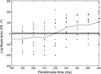
Evidence for feedback loops: Bayesian model comparison across subjects. Comparison of the model with backward connections (FB) against the model without (F), across all subjects over peristimulus windows of length 180–260 ms. The dots correspond to differences in log‐evidence for 11 subjects over time. The solid line shows the average log‐evidence differences over subjects. The points outside the gray zone imply very strong for FB over F for positive values and the converse for negative values.

Modeling‐Induced Responses

Evoked responses are just one aspect of brain responses to stimuli measured with M/EEG. Instead of averaging trial‐specific responses in time, an alternative strategy is to analyze induced responses, which are expressed in the average power following a time‐frequency decomposition [Bastiaansen and Hagoort, 2006; Donner et al., 2007; Gross et al., 2007; Gruber et al., 2006; Jensen et al., 2007; Klimesch, 1999]. The analysis of induced responses enables one to look at frequency responses localized in peristimulus time. Importantly, induced responses are sensitive to response components that are jittered with respect to stimulus onset [Tallon‐Baudry and Bertrand, 1999]. The principle of modeling M/EEG data‐features as the output of a network of sources can also be applied to induced responses. In this case, the DCM parameters encode the frequency response to exogenous input and coupling among different frequencies within and between sources [Chen et al., 2008]. These sorts of models may be useful for modeling abnormal synchronization in conditions like Parkinson's disease [Brown, 2007].

One key aspect of DCM for induced responses is that it differentiates between linear and nonlinear coupling, which corresponds to within and between‐frequencies coupling respectively. In this model, we do not use neural mass equations explicitly but a second‐order approximation. This gives a simpler and more phenomenological model, where the dynamics within‐ and between sources are governed by linear differential equations. This simplification allows us to test for nonlinear coupling directly by comparing models with and without between‐frequency coupling. In contrast to DCM for evoked responses, the spatial locations of the sources are not optimized and must be fixed a‐priori. This is because one has to estimate the spectral responses at each source before modeling these responses with DCM. This might influence the ensuing parameter estimates and renders their interpretation conditional on the sources chosen. The choice of sources could be based on a prior source localization step or other knowledge about the system in question; for details see [Chen et al., 2008]. As an illustration of DCM for induced responses, we analyzed EEG data acquired during face perception. We used a four‐source network: two sources in visual cortex (left visual LV and right visual RV), and two in the fusiform gyrus (LF and RF). As shown in Figure 5, DCM estimates coupling strengths as a function of frequency‐to‐frequency coupling. These matrices indicate how power at a specific frequency, in a source, will influence changes in the (same or different) frequencies in a target source. In the described version, DCM for induced responses is based on the average of the time‐frequency power spectra of single trial data. This means that the modeled data contains both induced and evoked responses, and that, for example, the alpha coupling, could be caused by either induced or evoked coupling. The example in Figure 5 shows that cross‐frequency coupling in spectral characterizations of EEG and MEG time‐series can be modelled, using a DCM, as dynamic broad‐band power changes as a consequence of linear and nonlinear coupling among brain sources.

Figure 5.

DCM for induced responses: results for nonlinear coupling between sources in a four‐source “face perception” network, where LV and RV are left and right visual sources, and LF and RF are left and right fusiform gyrus sources. The arrows show the directed connections from one source to another. The coupling strengths are represented as coupling functions of frequency × frequency. These show the effects the spectral density in one source has on the density in another. The right panel is a zoom‐in onto the low‐frequency coupling from source RV to RF and illustrates (nonlinear) alpha to beta coupling.

Modeling Steady State Responses

In the examples mentioned earlier, we dealt with evoked or induced responses as a function of peri‐stimulus time. However, one can also analyze the frequency profile (i.e., the spectrum) of data measured over hundreds of milliseconds to minutes under local stationarity assumptions. This frequency‐only data‐feature is useful when the exact timing of exogenous input is unknown or when the dynamics are purely endogenous; for example, in sleep research. Another example would be the comparison of steady‐state responses with and without the application of a drug. In such studies, one can posit that the responses have been induced by endogenous (or subcortical) input with a stationary statistical distribution, for example white noise. For steady‐state responses, a system can be understood as a filter with an associated transfer function. This function describes how any spectral input is shaped to produce spectral output. With DCM, we can use the concept of transfer functions by estimating both a physiologically plausible input distribution and the neuronal parameters determining the transfer function, given the output spectrum. This allows one to establish a mapping from the system parameters to the predicted frequency spectrum [Moran et al., 2007]4. As with evoked responses, this enables us to model differences between two or more spectra, acquired under different conditions, as consequences of specific parameter changes. These parameters might be intrinsic or extrinsic connections, but can also be, for example, excitatory rate constants which have a marked influence on the frequency spectrum [Moran et al., 2007]. The idea is to manipulate the (real) system; e.g., by experimental changes in the level of a neurotransmitter, model this change in terms of changes in specific DCM parameters, and then test hypotheses using Bayesian inference. This strategy has been applied to local field potentials (LFP) using one [Moran et al., 2008] and multiple sources [Moran et al., 2009]. Note that although we used LFP data, the same analysis can be applied to M/EEG data: LFP data do not require a sophisticated spatial electromagnetic forward model, i.e. lead‐field, but just a gain parameter on the electrode.

Inference on parameters

LFP recordings were taken from electrodes in the prefrontal cortex of two rat populations. Normal rats were reared in their normal social environment, while isolated rats were brought up in isolation. Isolation provides a well‐established model of sensorimotor abnormalities found in schizophrenic patients [Geyer et al., 1993]. The associated reduction in extracellular neurotransmitter levels usually leads to an up‐regulation of neurotransmitter uptake and a sensitization of post‐synaptic responses [Jabaudon et al., 1999]. As detailed in Moran et al. [ 2009], this suggests that the effects of isolation can be modeled as increase in the amplitude of the excitatory postsynaptic potentials elicited by presynaptic input (i.e., intrinsic coupling parameters).

The data set analyzed here was an average spectral response over a 10‐min period. During this period, the rats (two groups with six rats each) were behaving freely in their environment. Preprocessing involved a Fast Fourier Transform of the data, using the frequencies from 1 to 48 Hz. The inversion was performed separately using each rat's spectral response. The model could account for differences in spectral response, between the two groups, in various parameters. Population differences between their estimates were significant in the case of the excitatory synaptic kernel amplitude and a gain parameter that controls the mean firing rate; see Figure 6. As predicted, the intrinsic coupling parameters were larger in the isolated than in the control group. These results suggest a sensitization of post‐synaptic responses; i.e., an increase in the response amplitude, and an overall decrease in firing rate for the isolated group due to decreased gain in membrane potential to firing rate transfer (Fig. 6 bottom right). This neural mass parameter is a proxy for neuronal adaptation and highlights a greater adaptation in the isolated group. This is consistent with reduced levels of extracellular neurotransmitter, which were measured concurrently with the LFP recordings. For a detailed discussion of these results, see [Moran et al., 2008].

Figure 6.

Steady‐state response study using local field potentials and a single source DCM, results: The left panel shows the coupling parameters of the different cell groups within a source. The mean estimates of the excitatory intrinsic connectivity parameters γ₁,γ₂, and γ₃ are shown with the associated P‐value in parentheses (blue: control, red: isolated group). The right panels display the inferred excitatory impulse response function and sigmoid firing function for both groups (blue: control, red: isolated). See [Moran et al., 2008] for the definitions of the model parameters.

Inference on models

In another study, we showed that DCM for steady‐state responses can disambiguate the direction of coupling between two areas. We showed this using data from a fear‐learning study in mice [Seidenbecher et al., 2003], where mice were subject to a typical Pavlovian conditioning paradigm using acoustic tones (CS+ and CS−) and foot‐shock (US) [Moran et al., 2009]. After conditioning, mice display characteristic behavioural fear responses (freezing) to the CS+ alone [Brady, 2005]. The retrieval of negative memories, in response to a CS, has been found to be correlated with θ‐band coupling between the hippocampus (CA1) and the lateral nucleus of the amygdala (LA) [Seidenbecher et al., 2003]. The question here is: Using DCM, can we go beyond this assessment of undirected correlations between these two areas?

We performed a top‐down heuristic model search to identify the most likely model. This can be expedient when all possible combinations of connection types and architectures create an intractably large model search space. To do this, we sequentially optimized various model attributes, starting with complex models and removing connections to identify the best architecture [Moran et al., 2009] by ensuing the free‐energy bound on log‐model evidence always increased. The results suggested that the hippocampus and amygdala influence each other through bidirectional connections: Sounds which have been associated with shocks (CS+) lead to decreased directed amygdala‐hippocampal connectivity and increased hippocampal‐amygdala connectivity (as compared to neutral sounds, i.e. CS−) [Moran et al., 2009].

CONCLUSION AND FUTURE DIRECTIONS

In this review, we summarized the fundamental assumptions of dynamic causal modeling (DCM), a spatiotemporal model for EEG/MEG and LFP data. We illustrated the analysis principles using evoked, induced, and steady state responses.

DCM is not limited to the neural mass model [Jansen and Rit, 1995], or the ECD model described in this review. The current implementation of DCM supports the exchange of generative models, both temporal or neuronal and spatial. In Marreiros et al. [ 2009], we discuss replacing the neural‐mass with a mean‐field model of neuronal dynamics. Furthermore, for the spatial model, one can also relax the assumption that each source expresses itself as a focal ECD source and use small parameterised patches on the cortical surface [Daunizeau et al., submitted]. Critically, in DCM, all these models can be evaluated using Bayesian model comparison. In practice this enables one to compare various combinations of temporal and spatial models within DCM for a given data set. In addition, one can compare DCMs with different source and network configurations, see e.g. [Garrido et al., 2007b, 2008]. This gives the experimenter a wide range of potential models, which might explain the data. Although the search in this space of models might appear a daunting task, Bayesian model comparison, in combination with search heuristics, appears to be a reliable guide to identify the best models [Moran et al., 2009]. Changes in models are not only restricted to the form of the model; the network structure or the specifics of neuronal dynamics. One can also change the prior distributions on the model parameters. For example, one can use informed priors on the spatial parameters, to inform the model about expected source locations, or symmetry [Fastenrath et al., 2009].

Note that DCMs for M/EEG are necessarily complex, because they reflect the inherent complexity of the processes generating M/EEG data. The advantage of DCM is that hypotheses about the underlying functional architecture can be tested in a way that cannot be addressed with other approaches. The disadvantage is that a potentially large number of alternative models must be analyzed to establish the best model, using Bayesian model comparison. This takes a lot of computing time, because the inversion of each model can take several minutes (In some cases, as in the second study of steady‐state responses, an exhaustive search of model‐space is practically intractable). Furthermore, specifying the space of all plausible models requires a lot of neurophysiological and anatomical knowledge. The exploration of models space can only be heuristic, in the sense that one cannot test all possible models. The heuristics used to choose the models are usually motivated by a careful consideration of their validity, in relation to other knowledge and studies. In summary, users cannot test all possible models but should instead motivate their model search in a careful and qualified fashion; and interpret their findings in the light of the choices made. One useful guide to finding the right level of model complexity and detail is to ensure that the data contains evidence that can disambiguate among them. Practically, this is seen as meaningful differences in the log‐evidences. If all the models have the same evidence, this usually (but not necessarily) means that they are too complex or too simple for the data in question.

In our examples, we used at most two responses, which were acquired under two different conditions and modeled the difference in terms of changes in key parameters. However, DCM is not restricted to two responses; in general, we model differences between multiple responses as a function of changes in selected DCM parameters [Garrido et al., under review]. For example, one might vary a stimulus property or the difficulty of task over five levels, and assume that there is a linear relationship between difficulty and some connectivity parameter(s). This could be used to test hypotheses about how parametric manipulations (e.g., difficulty) are expressed at the level of neuronal computations and connectivity. These parametric modulations can be modelled in the current DCM software (see software note) in a straightforward fashion.

SOFTWARE NOTE

All procedures described in this note have been implemented as Matlab (MathWorks) code. The source code is freely available in the DCM and neural model toolboxes of the Statistical Parametric Mapping package (SPM8) at http://www.fil.ion.ucl.ac.uk/spm/.

REFERENCES

- Auranen T,Nummenmaa A,Hamalainen MS,Jääskeläinen IP,Lampinen J,Vehtari A,Sams M ( 2007): Bayesian inverse analysis of neuromagnetic data using cortically constrained multiple dipoles. Hum Brain Mapp 28: 979–994. [DOI] [PMC free article] [PubMed] [Google Scholar]
- Bastiaansen M,Hagoort P ( 2006): Oscillatory neuronal dynamics during language comprehension. Prog Brain Res 159: 179–196. [DOI] [PubMed] [Google Scholar]
- Bijma F,de Munck JC,Bocker KB,Huizenga HM,Heethaar RM ( 2004): The coupled dipole model: An integrated model for multiple MEG/EEG data sets. Neuroimage 23: 890–904. [DOI] [PubMed] [Google Scholar]
- Brady AT ( 2005): Hypoglutamatergia in the rat medial prefrontal cortex in two models of schizophrenia. Acta Neurobiol Exp 65: 29. [Google Scholar]
- Breakspear M,Roberts JA,Terry JR,Rodrigues S,Mahant N,Robinson PA ( 2006): A unifying explanation of primary generalized seizures through nonlinear brain modeling and bifurcation analysis. Cereb Cortex 16: 1296–1313. [DOI] [PubMed] [Google Scholar]
- Brown P ( 2007): Abnormal oscillatory synchronisation in the motor system leads to impaired movement. Curr Opin Neurobiol 17: 656–664. [DOI] [PubMed] [Google Scholar]
- Chen CC,Kiebel SJ,Friston KJ ( 2008): Dynamic causal modelling of induced responses. Neuroimage 41: 1293–1312. [DOI] [PubMed] [Google Scholar]
- Daunizeau J,Mattout J,Clonda D,Goulard B,Benali H,Lina JM ( 2006): Bayesian spatio‐temporal approach for EEG source reconstruction: Conciliating ECD and distributed models. IEEE Trans Biomed Eng 53: 503–516. [DOI] [PubMed] [Google Scholar]
- David O,Kiebel SJ,Harrison LM,Mattout J,Kilner JM,Friston KJ ( 2006): Dynamic causal modeling of evoked responses in EEG and MEG. Neuroimage 30: 1255–1272. [DOI] [PubMed] [Google Scholar]
- Doeller CF,Opitz B,Mecklinger A,Krick C,Reith W,Schroger E ( 2003): Prefrontal cortex involvement in preattentive auditory deviance detection: Neuroimaging and electrophysiological evidence. Neuroimage 20: 1270–1282. [DOI] [PubMed] [Google Scholar]
- Donner TH,Siegel M,Oostenveld R,Fries P,Bauer M,Engel AK ( 2007): Population activity in the human dorsal pathway predicts the accuracy of visual motion detection. J Neurophysiol 98: 345–359. [DOI] [PubMed] [Google Scholar]
- Fastenrath M,Friston KJ,Kiebel SJ ( 2009): Dynamical causal modelling for M/EEG: Spatial and temporal symmetry constraints. Neuroimage 44: 154–163. [DOI] [PubMed] [Google Scholar]
- Friston KJ,Harrison L,Penny W ( 2003): Dynamic causal modelling. Neuroimage 19: 1273–1302. [DOI] [PubMed] [Google Scholar]
- Friston K,Harrison L,Daunizeau J,Kiebel S,Phillips C,Trujillo‐Barreto N,Henson R,Flandin G,Mattout J ( 2008): Multiple sparse priors for the M/EEG inverse problem. Neuroimage 39: 1104–1120. [DOI] [PubMed] [Google Scholar]
- Gaillard AW ( 1988): Problems and paradigms in ERP research. Biol Psychol 26: 91–109. [DOI] [PubMed] [Google Scholar]
- Garrido MI,Kilner JM,Kiebel SJ,Friston KJ ( 2007a): Evoked brain responses are generated by feedback loops. Proc Natl Acad Sci USA 104: 20961–20966. [DOI] [PMC free article] [PubMed] [Google Scholar]
- Garrido MI,Kilner JM,Kiebel SJ,Stephan KE,Friston KJ ( 2007b): Dynamic causal modelling of evoked potentials: A reproducibility study. Neuroimage 36: 571–580. [DOI] [PMC free article] [PubMed] [Google Scholar]
- Garrido MI,Friston KJ,Kiebel SJ,Stephan KE,Baldeweg T,Kilner JM ( 2008): The functional anatomy of the MMN: A DCM study of the roving paradigm. Neuroimage 42: 936–944. [DOI] [PMC free article] [PubMed] [Google Scholar]
- Geyer MA,Wilkinson LS,Humby T,Robbins TW ( 1993): Isolation rearing of rats produces a deficit in prepulse inhibition of acoustic startle similar to that in schizophrenia. Biol Psychiatry 34: 361–372. [DOI] [PubMed] [Google Scholar]
- Gross J,Schnitzler A,Timmermann L,Ploner M ( 2007): Gamma oscillations in human primary somatosensory cortex reflect pain perception. PLoS Biol 5: e133. [DOI] [PMC free article] [PubMed] [Google Scholar]
- Gruber T,Giabbiconi CM,Trujillo‐Barreto NJ,Muller MM ( 2006): Repetition suppression of induced gamma band responses is eliminated by task switching. Eur J Neurosci 24: 2654–2660. [DOI] [PubMed] [Google Scholar]
- Jabaudon D,Shimamoto K,Yasuda‐Kamatani Y,Scanziani M,Gahwiler BH,Gerber U ( 1999): Inhibition of uptake unmasks rapid extracellular turnover of glutamate of nonvesicular origin. Proc Natl Acad Sci USA 96: 8733–8738. [DOI] [PMC free article] [PubMed] [Google Scholar]
- Jansen BH,Rit VG ( 1995): Electroencephalogram and visual evoked potential generation in a mathematical model of coupled cortical columns. Biol Cybern 73: 357–366. [DOI] [PubMed] [Google Scholar]
- Jemel B,Achenbach C,Muller BW,Ropcke B,Oades RD ( 2002): Mismatch negativity results from bilateral asymmetric dipole sources in the frontal and temporal lobes. Brain Topogr 15: 13–27. [DOI] [PubMed] [Google Scholar]
- Jensen O,Kaiser J,Lachaux JP ( 2007): Human gamma‐frequency oscillations associated with attention and memory. Trends Neurosci 30: 317–324. [DOI] [PubMed] [Google Scholar]
- Jun SC,George JS,Plis SM,Ranken DM,Schmidt DM,Wood CC ( 2006): Improving source detection and separation in a spatiotemporal Bayesian inference dipole analysis. Phys Med Biol 51: 2395–2414. [DOI] [PubMed] [Google Scholar]
- Kiebel SJ,David O,Friston KJ ( 2006): Dynamic causal modelling of evoked responses in EEG/MEG with lead field parameterization. Neuroimage 30: 1273–1284. [DOI] [PubMed] [Google Scholar]
- Kiebel SJ,Garrido MI,Friston KJ ( 2007): Dynamic causal modelling of evoked responses: The role of intrinsic connections. Neuroimage 36: 332–345. [DOI] [PubMed] [Google Scholar]
- Kiebel SJ,Daunizeau J,Phillips C,Friston KJ ( 2008a): Variational Bayesian inversion of the equivalent current dipole model in EEG/MEG. Neuroimage 39: 728–741. [DOI] [PubMed] [Google Scholar]
- Kiebel SJ,Garrido MI,Moran RJ,Friston KJ ( 2008b): Dynamic causal modelling for EEG and MEG. Cogn Neurodyn 2: 121–136. [DOI] [PMC free article] [PubMed] [Google Scholar]
- Klimesch W ( 1999): EEG alpha and theta oscillations reflect cognitive and memory performance: A review and analysis. Brain Res Rev 29: 169–195. [DOI] [PubMed] [Google Scholar]
- Marreiros AC,Daunizeau J,Kiebel SJ,Friston KJ ( 2008): Population dynamics: Variance and the sigmoid activation function. Neuroimage 42: 147–157. [DOI] [PubMed] [Google Scholar]
- Marreiros AC,Kiebel SJ,Daunizeau J,Harrison LM,Friston KJ ( 2009): Population dynamics under the Laplace assumption. Neuroimage 44: 701–714. [DOI] [PubMed] [Google Scholar]
- Moran RJ,Kiebel SJ,Stephan KE,Reilly RB,Daunizeau J,Friston KJ ( 2007): A neural mass model of spectral responses in electrophysiology. Neuroimage 37: 706–720. [DOI] [PMC free article] [PubMed] [Google Scholar]
- Moran RJ,Stephan KE,Kiebel SJ,Rombach N,O'Connor WT,Murphy KJ,Reilly RB,Friston KJ ( 2008): Bayesian estimation of synaptic physiology from the spectral responses of neural masses. Neuroimage 42: 272–284. [DOI] [PMC free article] [PubMed] [Google Scholar]
- Moran RJ,Stephan KE,Seidenbecher T,Pape HC,Dolan RJ,Friston KJ ( 2009): Dynamic causal models of steady‐state responses. Neuroimage 44: 796–811. [DOI] [PMC free article] [PubMed] [Google Scholar]
- Mosher JC,Leahy RM,Lewis PS ( 1999): EEG and MEG: Forward solutions for inverse methods. IEEE Trans Biomed Eng 46: 245–259. [DOI] [PubMed] [Google Scholar]
- Nummenmaa A,Auranen T,Hamalainen MS,Jääskeläinen IP,Lampinen J,Sams M,Vehtari A ( 2007a): Hierarchical Bayesian estimates of distributed MEG sources: Theoretical aspects and comparison of variational and MCMC methods. Neuroimage 35: 669–685. [DOI] [PubMed] [Google Scholar]
- Nummenmaa A,Auranen T,Hamalainen MS,Jääskeläinen IP,Sams M,Vehtari A,Lampinen J ( 2007b): Automatic relevance determination based hierarchical Bayesian MEG inversion in practice. Neuroimage 37: 876–889. [DOI] [PMC free article] [PubMed] [Google Scholar]
- Opitz B,Rinne T,Mecklinger A,von Cramon DY,Schroger E ( 2002): Differential contribution of frontal and temporal cortices to auditory change detection: fMRI and ERP results. Neuroimage 15: 167–174. [DOI] [PubMed] [Google Scholar]
- Penny WD,Kilner J,Blankenburg F ( 2007): Robust Bayesian general linear models. Neuroimage 36: 661–671. [DOI] [PubMed] [Google Scholar]
- Penny WD,Stephan KE,Mechelli A,Friston KJ ( 2004): Comparing dynamic causal models. Neuroimage 22: 1157–1172. [DOI] [PubMed] [Google Scholar]
- Rinne T,Alho K,Ilmoniemi RJ,Virtanen J,Naatanen R ( 2000): Separate time behaviors of the temporal and frontal mismatch negativity sources. Neuroimage 12: 14–19. [DOI] [PubMed] [Google Scholar]
- Rodrigues S,Terry JR,Breakspear M ( 2006): On the genesis of spike‐wave oscillations in a mean‐field model of human thalamic and corticothalamic dynamics. Phys Lett A 355: 352–357. [Google Scholar]
- Salmelin RH,Hamalainen MS ( 1995): Dipole modelling of MEG rhythms in time and frequency domains. Brain Topogr 7: 251–257. [DOI] [PubMed] [Google Scholar]
- Sams M,Paavilainen P,Alho K,Naatanen R ( 1985): Auditory frequency discrimination and event‐related potentials. Electroencephalogr Clin Neurophysiol 62: 437–448. [DOI] [PubMed] [Google Scholar]
- Scherg M,von Cramon D ( 1985): Two bilateral sources of the late AEP as identified by a spatio‐temporal dipole model. Electroencephalogr Clin Neurophysiol 62: 32–44. [DOI] [PubMed] [Google Scholar]
- Seidenbecher T,Laxmi TR,Stork O,Pape HC ( 2003): Amygdalar and hippocampal theta rhythm synchronization during fear memory retrieval. Science 301: 846–850. [DOI] [PubMed] [Google Scholar]
- Sotero RC,Trujillo‐Barreto NJ,Iturria‐Medina Y,Carbonell F,Jimenez JC ( 2007): Realistically coupled neural mass models can generate EEG rhythms. Neural Comput 19: 478–512. [DOI] [PubMed] [Google Scholar]
- Sotero RC,Trujillo‐Barreto NJ ( 2008): Biophysical model for integrating neuronal activity, EEG, fMRI and metabolism. Neuroimage 39: 290–309. [DOI] [PubMed] [Google Scholar]
- Sussman E,Winkler I ( 2001): Dynamic sensory updating in the auditory system. Brain Res Cogn Brain Res 12: 431–439. [DOI] [PubMed] [Google Scholar]
- Tallon‐Baudry C,Bertrand O ( 1999): Oscillatory gamma activity in humans and its role in object representation. Trends Cogn Sci 3: 151–162. [DOI] [PubMed] [Google Scholar]
- Winkler I,Karmos G,Naatanen R ( 1996): Adaptive modeling of the unattended acoustic environment reflected in the mismatch negativity event‐related potential. Brain Res 742: 239–252. [DOI] [PubMed] [Google Scholar]
- Zumer JM,Attias HT,Sekihara K,Nagarajan SS ( 2007): A probabilistic algorithm integrating source localization and noise suppression for MEG and EEG data. Neuroimage 37: 102–115. [DOI] [PubMed] [Google Scholar]
- Zumer JM,Attias HT,Sekihara K,Nagarajan SS ( 2008): Probabilistic algorithms for MEG/EEG source reconstruction using temporal basis functions learned from data. Neuroimage 41: 924–940. [DOI] [PMC free article] [PubMed] [Google Scholar]