Oscillatory response function: Towards a parametric model of rhythmic brain activity

Abstract

Rhythmic brain activity, measured by magnetoencephalography (MEG), is modulated during stimulation and task performance. Here, we introduce an oscillatory response function (ORF) to predict the dynamic suppression–rebound modulation of brain rhythms during a stimulus sequence. We derived a class of parametric models for the ORF in a generalized convolution framework. The model parameters were estimated from MEG data acquired from 10 subjects during bilateral tactile stimulation of fingers (stimulus rates of 4 Hz and 10 Hz in blocks of 0.5, 1, 2, and 4 s). The envelopes of the 17–23 Hz rhythmic activity, computed for sensors above the rolandic region, correlated 25%–43% better with the envelopes predicted by the models than by the stimulus time course (boxcar). A linear model with separate convolution kernels for onset and offset responses gave the best prediction. We studied the generalizability of this model with data from 5 different subjects during a separate bilateral tactile sequence by first identifying neural sources of the 17–23 Hz activity using cortically constrained minimum norm estimates. Both the model and the boxcar predicted strongest modulation in the primary motor cortex. For short‐duration stimulus blocks, the model predicted the envelope of the cortical currents 20% better than the boxcar did. These results suggest that ORFs could concisely describe brain rhythms during different stimuli, tasks, and pathologies. Hum Brain Mapp, 2010. © 2009 Wiley‐Liss, Inc.

INTRODUCTION

Rhythmic activity is observed in electroencephalographic (EEG) and magnetoencephalographic (MEG) measurements of brain function at characteristic frequencies and brain regions. Spontaneous rhythms are prominent particularly in the absence of external stimuli. The rhythms are perturbed from their resting level during processing of sensory stimuli, task performance, changes in alertness, or brain disease, and hence may be considered as signatures of information processing in the brain.

The rolandic mu rhythm is suppressed during motor action, motor imagery, and somatosensory stimulation. Both the 10‐Hz and the 20‐Hz frequency bands of the mu rhythm return to baseline levels after the stimulation or task ends; however, some characteristic differences have been reported. First, the 20‐Hz component rebounds earlier and faster than the 10‐Hz component. Second, the source of the 20‐Hz component reflects the moved body part according to the somatotopy in the primary motor cortex, whereas the 10‐Hz component does not—rather, it arises from the hand area of the somatosensory cortex [Salmelin and Hari, 1994; Salmelin et al., 1995].

The mu rhythm has been used to probe the state of the sensorimotor system under various perceptual states; for instance, mu suppresses weakly during motor imagery [Schnitzler et al., 1997] and observation of motor action [Hari et al., 1998]. Precentral 20‐Hz and postcentral 10‐Hz EEG rhythms seem to correlate inversely with the blood‐oxygen‐level dependent (BOLD) signal [Ritter et al., 2009]. Different levels of correlation between different EEG rhythms and resting‐state networks of BOLD activity have also been reported [Mantini et al., 2007]. The reactivity of various rhythms has thus become increasingly important in the study of human cognitive function.

Although several studies have already related various tasks and stimuli to specific modulations of brain rhythms, the available descriptions are largely qualitative. To unify this information, a quantitative, parametric model of the relationship between the environment and brain rhythms is essential. With such a model, it would be possible to predict the responses of the brain rhythms to novel events, compare the responses to different events, and quantify these differences in terms of the model parameters. Such a parametric model would also facilitate a hypothesis‐driven approach to understanding the functional significance of the rhythmic activity, and it could serve as a benchmark against which future quantitative models could be compared.

Early generative models of neural population dynamics (neural mass models) [Lopes da Silva et al., 1974; Zetterberg, et al. 1978] serve as precedents for interpretation of the generative process of brain rhythms and for the predictive modeling of their state as a function of stimulus or task. The neural mass model of Jansen and Rit [ 1995] describes the generation of the alpha rhythm by means of interacting populations of pyramidal neurons, excitatory interneurons, and inhibitory interneurons. In this work, the transformation of synaptic input into postsynaptic potentials was modeled by a linear convolution, with different impulse response functions for excitatory and inhibitory synapses. For each neuronal population, the net postsynaptic potential was transformed to an average firing rate by a sigmoid function. The authors showed that with uniformly distributed white noise as the external input to the pyramidal neurons, the time course of the average of postsynaptic potentials of the pyramidal neuron population resembled the alpha rhythm observed in EEG recordings. A variant of this model has been proposed by David and Friston [ 2003] as a building block for dynamic causal modeling (DCM), a framework for discovering causal relationships between different neuronal populations.

These neural mass models have been typically generative (where the goal of modeling is to understand the biophysical process by which the rhythm of interest is generated) as opposed to predictive (where the goal is to predict the state of the rhythm under specific conditions).

The neural mass models have largely focused on the alpha rhythm whereas the literature on generative models of the mu rhythm is more sparse. Recently, Jones et al. [ 2007a] proposed a biophysically realistic laminar network model of the primary somatosensory cortex (SI) to predict the evoked MEG response to tactile stimulation. On the basis of simulations, the same authors [Jones et al., 2007b] suggested that the mu rhythm may be produced by feedforward/feedback drive from/to the thalamus to/from the somatosensory cortical regions at 10 Hz. This bottom‐up model, similar to the generative neural mass models, requires prior knowledge and assumptions about the underlying generative process.

Black‐box models (also referred to as data‐driven or phenomenological models) ignore the biophysical processes underlying the observed rhythmic activity, and being relatively assumption‐free they are sometimes useful for prediction. Such a parametric model of the event‐related modulations of the spectral features of the mu rhythm was proposed by Krusienski et al. [ 2007] to provide a tool for continuous tracking of the EEG mu rhythm for a brain‐computer interface.

Altogether, most of the literature on modeling of electrophysiological brain rhythms concerns descriptive rather than predictive models. To complement this body of work, here we introduce a framework for a predictive model of envelope dynamics with potential applications in locating cortical generators of brain rhythms, as well as in characterizing their dynamics as a function of stimuli, and subjects in health and disease. Specifically, we introduce a predictive model of the envelope dynamics of the 20‐Hz component of the rolandic mu rhythm. The inspiration for the model comes from the analysis of functional magnetic resonance imaging (fMRI) data, where a linear transformation employing a hemodynamic response function (HRF) is used to predict the time course of the hemodynamic response to a stimulus or task. Appropriately, the model presented here employs a transformation called the oscillatory response function (ORF). Since the rebound of the envelope above the resting level is associated only with the end of the stimulus or task, the reactivity of the 20‐Hz mu‐rhythm envelope should be considered nonlinear. Therefore, we employed generalized convolution [Schetzen, 2006] for modeling the envelope; within this framework, any nonlinear, time‐invariant system can be modeled. We obtained the model parameters using a supervised machine learning approach, specifically by minimizing the mean‐squared prediction error within a training dataset obtained from healthy subjects, consisting of known stimulus sequences as inputs and envelopes of the mu rhythm as outputs. The model parameters were then used to predict the envelope dynamics in an independent testing dataset.

MATERIALS AND METHODS

Subjects

Fourteen healthy adults (six females, eight males; mean age, 28 years; range, 22–41) participated in the study after written informed consent. Of these, ten subjects participated in the training paradigm and five in the test paradigm (one subject taking part in both). The recordings were approved by the Ethics Committee of the Helsinki and Uusimaa Hospital District (protocols No. 9‐49/2000 and No. 95/13/03/00/2008), granted to N. Forss and R. Hari.

Stimuli

For both training and testing datasets, tactile stimuli were delivered using pneumatic diaphragms at the fingertips of both hands. The stimuli for the test dataset were designed to be informative about the generalizability of the estimated model as a function of stimulus parameters. We employed a design with alternating stimulus and rest blocks (see Fig. 1) and bilateral stimulation to engage the somatosensory cortex of both hemispheres. Within a stimulus block, the tactile pulses were presented in a random order under the constraint that homologous fingers were stimulated simultaneously. The timing of stimulus delivery was controlled using Presentation Software (version 0.81, Neurobehavioral Systems Inc., Albany, CA, USA). A 2‐min recording without a subject was conducted after the experiment for the estimation of noise statistics. The experiments for model training and testing differed in terms of the number of fingers stimulated, the duration of the stimulus blocks, and the frequency of the stimulus trains, as described below.

Figure 1.

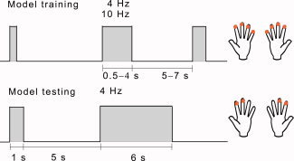
Stimulus presentation for model training (above) and testing (below). Both sequences comprised blocks of tactile stimuli (presented either at 4 or 10 Hz for model training, and at 4 Hz for model testing), interspersed by rest periods. The stimuli were delivered to fingers 2–5 in the training set and to fingers 2–3 in the testing set. [Color figure can be viewed in the online issue, which is available at www.interscience.wiley.com.]

Experimental Design for Model Training

The session consisted of two 13‐min sequences of pneumotactile stimulus trains. In a single train, the stimuli were given at either 4 Hz (Sequence 1) or 10 Hz (Sequence 2) as shown in Figure 1. All fingers except the thumb were stimulated. Each sequence consisted of 25 stimulus blocks of four different durations (0.5, 1, 2, and 4 s), occurring in a random order. The rest blocks were of five different durations (5.0, 5.5, 6.0, 6.5, and 7.0 s).

Experimental Design for Model Testing

This session comprised one 11‐min sequence with pneumotactile stimuli at 4 Hz. Each stimulus sequence comprised 40 trials, each of them with a short stimulus block (1 s), a rest block (5 s), a long stimulus block (6 s), and another rest block (5 s). Only the index and middle fingers were stimulated (see Fig. 1).

Measurements

MEG data were acquired with a 306‐channel MEG system (Elekta Neuromag Oy, Helsinki, Finland), bandpass‐filtered to 0.03‐200 Hz and digitized at 600 Hz. The training and testing datasets were acquired at different measurement sites at the Helsinki University of Technology; the training dataset in a three‐layer shielded room and the testing dataset in a two‐layer shielded room equipped with active compensation.

During the MEG recording, four small coils, whose locations had been digitized with respect to anatomical landmarks, were briefly energized to determine the subject's head position with respect to the MEG sensors. For the training dataset, the head position was monitored continuously during the measurement, whereas in the testing paradigm, the head position was measured only in the beginning of each sequence. Anatomical MRIs were obtained using a 3‐T General Electric Signa MRI scanner (Milwaukee, WI) at the AMI Centre of the Helsinki University of Technology.

Generalized Convolution Models

The Volterra series

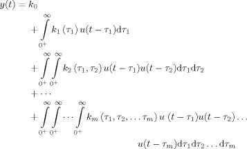
The output y(t) of a linear time‐invariant (LTI) system can be modeled as a convolution of an input u(t) with an impulse response function (IRF) k(t), defined as the system output to an infinitesimally brief input δ(t). Linear convolution can be extended to a generalized convolution framework in which any nonlinear, time‐invariant system can be expressed as an infinite series of functionals (the Volterra series) constructed by multiple convolutions of the input [Schetzen, 2006]. For the input u(t), the output y(t) is given by the Volterra series as

(1)

where k _m is called the m‐th‐order Volterra kernel, and k ₀ is a constant which captures the time‐invariant offset. The first‐order kernel k ₁ represents the linear unit impulse response of the system, similar to the IRF in the linear convolution framework. Similarly, the second‐order kernel k ₂ is a two‐dimensional function of time and represents the system response to two unit impulses applied at different points in time. In practice, the Volterra series is often truncated to the second order because the amount of data required to estimate each higher‐order kernel scales exponentially with the model order [Victor, 2005].

Generalized Convolution and the mu‐Rhythm Envelope

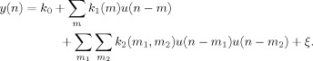
The discrete time representation of the univariate model, with the Volterra series truncated to the second order, is given by

(2)

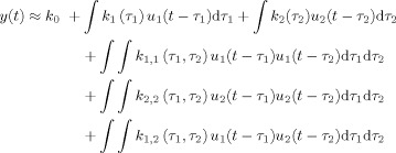
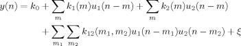
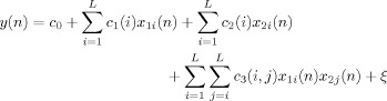
The input u(n) is a step function encoding stimulus onset and offset (boxcar). The output y(n) is the envelope of the mu rhythm. A residual term ξ represents the modeling error due to series truncation. By extension, the Volterra series can also be applied to bivariate models, i.e., to models with two inputs. The output of the second‐order Volterra series expansion for a bivariate model

(3)

where the first two integrals represent the linear part of the response to inputs u ₁(t) and u ₂(t). The next two integrals represent the self terms of the nonlinear part of the response, i.e. the response due to the interaction of inputs with themselves. The last integral represents the cross term, i.e. the response due to the interaction between the two inputs.

The rationale for adopting a bivariate model was as follows. The reactivity of the mu rhythm suggests that the stimulus onset and offset events are processed differently, because the onset is followed by a suppression that continues during the stimulation, and the offset is followed by a rebound above the prestimulus level. Accordingly, a model with two inputs was adopted: u ₁(t), a boxcar function encoding stimulus onset and offset as in the univariate model, and u ₂(t) an impulse function encoding stimulus offset alone; and one output y(t) representing the mu rhythm envelope. The impulse function u ₂(t) may be defined in terms of the step function u ₁(t) as

(4)

where {.}₊ denotes half‐wave rectification.

Further, it was assumed that for the applied stimulus train durations and inter‐train intervals, the successive onsets (offsets) do not interact, i.e. that the rebound after a stimulus train depends on the duration of the current stimulus train only; not on the previous stimulus trains. Accordingly, we dropped the self terms in Eq. (3). The discrete‐time representation of the resulting bivariate model is thus given by

(5)

where k ₁(m) is called the onset kernel, k ₂(m) the offset kernel, and k ₁₂(m ₁, m ₂) the interaction kernel. We estimated both the univariate [Eq. (2)] and bivariate [Eq. (5)] models from the training dataset.

Estimation of Volterra kernels

A parametric approach to estimate the Volterra kernels was first suggested by Wiener [ 1958] and has since undergone a number of modifications [Marmarelis, 1993; Watanabe and Stark, 1975]. The essential idea is to expand the kernels as functions of an orthonormal basis, so that it is sufficient to estimate the coefficients of the basis functions, thus reducing the number of model parameters.

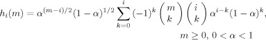
The discrete‐time Laguerre basis set (see Fig. 2) is ideally suited to capture the morphology of the mu‐rhythm envelope. The Laguerre basis [Back and Tsoi, 1996; Broome, 1965; Marmarelis, 1993] is also favorable because of its parsimony; the entire basis set is completely specified by a single parameter α. The i‐th discrete‐time Laguerre function is computed in the closed form as

(6)

where α is the discrete‐time Laguerre parameter, or the Laguerre pole, which determines the rate of the exponential decay of the functions. As a general principle, the number of basis functions must be large enough to sufficiently span the signal space and, at the same time, small enough to minimize over‐learning and keep the estimation numerically feasible.

Figure 2.

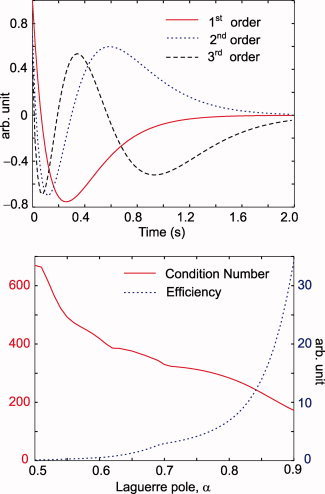
The first three discrete Laguerre basis functions with a 2‐s support (above). The Laguerre pole α = 0.8. The condition number and efficiency (see text) of the design matrix X, plotted as a function of α (below). [Color figure can be viewed in the online issue, which is available at www.interscience.wiley.com.]

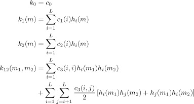
The kernels are represented as Laguerre expansions with coefficients c ₀, c ₁, c ₂, c ₃ as

(7)

where L is the number of Laguerre basis functions. By substitution, Eq. (5) reduces to

(8)

where

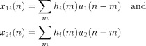Eq. (8) can be written in a matrix form as Y = Xβ, where

(9)

and

(10)

The coefficients are then obtained as the least‐squares estimate of β,

(11)

where W is a diagonal matrix with entries as reciprocals of the data variance. This approach closely follows the least‐squares estimation proposed by Marmarelis [ 1993]. For an adaptation of the technique to estimate the hemodynamic response function from fMRI data, see Lee et al. [ 2004].

Data Analysis

Estimation of sensor‐ and source‐space envelopes of the mu rhythm

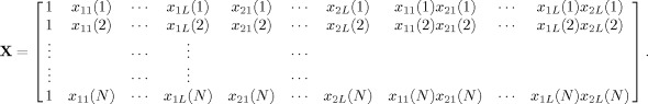
The continuous, raw MEG data were low‐pass‐filtered to 50 Hz, and downsampled to a sampling rate of 150 Hz. External interference was removed and head movements were compensated for using the signal space separation (SSS) method [Taulu and Kajola, 2005]. For one subject, whose recordings contained slowly varying artifacts, the temporal extension (tSSS) of the method was applied [Taulu and Simola, 2006]. Next, the signals were band‐limited to 17–23 Hz (the typical range of the 20‐Hz component) using a Butterworth FIR filter with −3‐dB cut‐offs at 15.4 Hz and 24.6 Hz, a transition band of 4.4 Hz, and a stopband attenuation of −85 dB. Given that the envelopes vary slowly compared with the signals, the data were further down‐sampled to 50 Hz for computational feasibility of the modeling process. From the training dataset, the instantaneous amplitude was computed as the magnitude of the complex Hilbert analytic signal. Figure 3 shows the envelopes at representative gradiometer channels, selected individually for the largest mu rhythm modulation, for all 10 subjects over the left rolandic region. Representative channels were also individually selected from the right rolandic regions in an identical manner (not shown). A clear suppression–rebound oscillatory response was seen in all subjects, except in S1, S4, and S7. These sensor‐space envelopes were used for estimation of model parameters from the training set.

Figure 3.

Envelopes of the 17–23 Hz signals at the representative left hemisphere channels used for model estimation. Data from all 10 subjects (S1–S10), for both stimulus presentation rates (4 Hz and 10 Hz) and all four stimulus durations (0.5, 1, 2, and 4 s) are shown.

The test dataset was preprocessed identically as the training dataset, except that the cortical current envelopes were further down sampled to 10 Hz. The envelopes of the cortical sources were estimated using a cortically constrained ℓ₂ minimum norm estimate as follows. Individual anatomical MRIs were segmented for the cortical mantle using the Free Surfer software package (http://surfer.nmr.mgh.harvard.edu, Martinos Center for Biomedical Imaging, Massachusetts General Hospital) and a source space with a 15‐mm spacing between the adjacent sources along the cortical surface was defined. A forward solution was computed for each source point using a boundary element conductor model for the cranium and taking into account the position of the head with respect to the MEG sensors. Noise covariance was estimated using the 2‐min recording without a subject at the end of each session. No regularization was applied to the noise covariance. A depth‐weighted, minimum‐norm inverse operator [Dale et al., 2000] was computed with a loose orientation constraint favoring source currents perpendicular to the local cortical surface by a factor of 2.5 with respect to the currents along the surface [Lin et al., 2006]. Using the inverse operator, the Hilbert analytic signal was projected on to the cortex. Finally, the cortical envelope was computed by taking the magnitude of the complex‐valued analytic signal at each cortical location. These source‐space envelopes from the test set were used to validate the model estimated from sensor‐space envelopes in the training set. It is sufficient to estimate the model parameters from sensor‐space signals, because the minimum‐norm inverse projection is linear and thus preserves the essential spatiotemporal characteristics of the envelope.

Model fitting

Both univariate and bivariate models were fit to the training dataset. For the bivariate model, both a linear (1st‐order Volterra expansion) model involving only the onset and offset kernels, and a nonlinear (2nd‐order Volterra expansion) model including the interaction kernel, were fit to the envelope. For each stimulus train rate, envelopes were averaged across trials for each stimulus duration using a 2‐s prestimulus and a 2‐s poststimulus baseline. Trials with MEG signals exceeding 3 pT/cm, and EOG signals exceeding 100 μV, apparently caused by nonphysiological artifacts and eye blinks, were rejected. A linear trend (across each stimulus block) was removed from the data prior to averaging. Blocks of each duration and stimulus rate were averaged together and these averages were concatenated. For each stimulus rate, a representative rolandic channel was selected by visual inspection from both the left and the right hemisphere for modeling. Supporting Information Figure S1 shows data from subject S3.

To avoid temporal discontinuities in the model output at the stimulus onsets and offsets, the inputs to the model were smoothed using a 200‐ms moving average kernel. For the basis set, three Laguerre functions (L = 3) were used, thus requiring one parameter for the baseline level, L = 3 parameters for the onset kernel, L = 3 parameters for the offset kernel and L(L+1)/2 = 6 parameters for the interaction kernel. In addition, the hyperparameter α was allowed to vary freely. Thus, 11 parameters were employed for the univariate model, 14 for the nonlinear bivariate model, and 8 for the linear bivariate model. The temporal support of the kernels was chosen to be 2 s (100 samples). The choice of the number of basis functions was practically motivated: to restrict the parameters to as few as possible, and to keep the design matrix sufficiently high‐rank, so that parameter estimation was numerically feasible. Test runs on MEG data from a single subject suggested that L = 2 was too few to capture the morphology of the mu reactivity, while L = 4 resulted in a ill‐conditioned design matrix. In this sense, L = 3 seemed to be an optimal choice.

Theoretically, although an orthogonal basis of high cardinality can explain any function, the choice of the Laguerre pole α is critical for obtaining a good model fit with a few Laguerre basis functions [Campello et al., 2004]. Hence, we allowed α to vary as a free parameter. The initial choice was such that the basis functions remained orthogonal within the 2‐s support and the design matrix X in Eq. (10) was numerically well conditioned. Specifically, for efficient estimation of the parameters, it was desirable for X to have a low condition number, i.e. the ratio of the largest to the smallest singular value. Figure 2 shows the basis functions with α = 0.8 for a 2‐s support and a plot of efficiency and condition number as a function of α. Efficiency is a statistical measure defined as the reciprocal of the trace of the covariance matrix of X, and it is inversely related to the variance of the estimator [Dale, 1999].

The hyperparameter α was initialized to 0.8 and an initial guess for the coefficients for the basis functions was obtained using a weighted least‐squares fit. With this initial guess, the coefficients, together with α, were then considered as free parameters in an iterative nonlinear optimization algorithm (Nelder‐Mead simplex search) which minimized the weighted mean‐square prediction error.

Inter‐subject variability

To obtain a predictive model with good generalizability, we averaged all individually determined model parameters across the two stimulus rates, the two channels and the 10 subjects yielding a group average across 40 conditions.

We studied the variability among model parameters derived individually from the training set in two ways. First, we tested the parameters for statistically significant differences between (a) left and right hemispheres and (b) 10‐Hz and 4‐Hz stimulus train rates (significance level P = 0.05, Bonferroni‐corrected; N = 8, 14, and 11 for the linear bivariate, nonlinear bivariate, and univariate models, respectively). Second, we computed from these parameters, the predicted response to a hypothetical stimulus of 1‐s duration to assess the variability of their predictive power. As a similarity metric between individual predictions, we calculated all possible pairwise correlations (from 40 conditions resulting in 780 pairs) between the individual model predictions and studied their distribution. We computed this distribution for each of the three models, viz. the univariate, the linear bivariate and the nonlinear bivariate.

Model diagnostics

The three different models (univariate, linear bivariate, and nonlinear bivariate) may be compared by the correlation coefficient between the data from the training set and each model's predictions of them. An average measure of correlation across the 40 conditions was computed with a leave‐one‐out cross‐validation approach. Here, the parameters from 39 of the 40 conditions were averaged as described above and used to predict the envelope of the remaining condition. The prediction was then repeated for all conditions, and the mean correlation coefficient between model predictions and data was computed across all conditions. The three models were compared on the grounds of both the predictive power (model fit) and parameter parsimony.

Model validation

Any truly useful model must be generalizable. Thus, a test dataset was acquired to investigate the generalizability (i) across subjects, (ii) across acquisition setups (ambient noise spectra and covariance), and (iii) across stimulus durations. The validation approach was designed to further test the model generalizability (iv) from sensor to source space and (v) from event‐related averages to unaveraged envelopes. To this end, the Hilbert envelope was calculated in the source space of a cortically constrained minimum norm estimate from the testing dataset, and fit to two different general linear models (GLMs), each with a single regressor and a constant term. As regressors, we applied both the stimulus time course and the oscillatory response predicted by the best performing model from the training set as determined above. The GLM allows generalizations to unaveraged envelopes in the sense that it is applicable to arbitrary stimulus designs with no requirements that the stimulus trains are of equal durations (which would be a necessary condition for averaging across stimulus trains).

GLMs were fit separately for each subject. We defined the ratio between the GLM coefficient of the regressor and that of the constant term as the modulation depth (MD). In communication theory, modulation depth is a metric for the extent of modulation of a variable around its base level. We defined the resulting map of MDs over the entire brain surface as a modulation depth map (MDM). Only source points statistically significantly (P < 0.05, Bonferroni‐corrected for an upper limit of 5,000 uncorrelated source points) predicted by the model were retained in the MDMs. Further, among the statistically significant source points, only those with the largest MDs (top 1%) were visualized; this thresholding was necessary because of the inherent spread of MNE which the statistical testing alone cannot take into account. Since the mean number of source points among the test subjects was 2,243, the Bonferroni‐corrected significance level was considered appropriate. It is worth noting that source points are assumed uncorrelated; if their correlations are taken into account, the applied significance level could be less conservative. Single‐subject maps were projected to the Free Surfer Average (FSA) brain and subsequently averaged across subjects.

To compare the predicted (by the model) and source estimates (by the minimum‐norm) of the measured cortical current envelopes in each subject, we isolated the source point with the maximum MD for further analysis. The cortical envelope for the selected source point was averaged separately across the 1‐ and 6‐s stimulus trials. Correlation coefficients were computed between the averaged envelopes and the predictions of the best model, as well as the stimulus time course, for comparison.

RESULTS

Inter‐Subject Variability

The model parameter sets (α and the β's) derived from the training data were not found to be statistically significantly different between the left and right hemispheres. However, some significant differences were observed between the 10‐Hz and 4‐Hz conditions for the univariate and the linear bivariate model. For the univariate model, α was found to be greater for the 10‐Hz than the 4‐Hz condition (P = 0.014). For the linear bivariate model, one parameter related to the onset kernel: c ₃ (P = 0.012) in Eq. (9) was found to be significantly different between 10‐ and 4‐Hz conditions.

Figure 4 shows the variability of the model predictions within four subgroups, viz. predicted left and right hemisphere responses to 4‐ and 10‐Hz stimulus trains. The subaverages of individual model predictions of the response to a hypothetical 1‐s stimulus train, estimated from the parameters of the 10 training‐set subjects, are shown across these subgroups. The histograms of the pairwise correlations between individual model predictions, computed as a measure of variability across conditions (40 conditions, resulting in 780 pairs for each model) are shown as insets. Half the pairwise correlations between individual model predictions exceeded 0.87, 0.71, and 0.81, for the linear bivariate, the nonlinear bivariate, and the univariate models, respectively.

Figure 4.

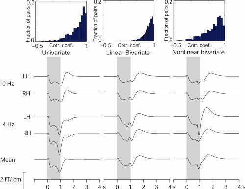
Variability of model predictions across subjects and categories. The individually determined parameters from the training set were first used to predict envelope dynamics for a hypothetical 1‐s test stimulus. These individual predictions were averaged separately for all 10 subjects over four subgroups (10‐ and 4‐Hz stimulus rates; left‐ and right‐hemisphere channels, denoted LH and RH, respectively). The insets on top show histograms of pairwise correlation‐coefficients (40 conditions, resulting in the binomial coefficient ⁴⁰ C ₂ = 780 pairs) between model predictions. [Color figure can be viewed in the online issue, which is available at www.interscience.wiley.com.]

Figure 5 shows the individual predictions of the envelope modulation during a test stimulus consisting of the four durations in the experiment (0.5, 1, 2, and 4 s) by the parameters of the linear bivariate model. Individual predictions as well as subaverages across the 10‐Hz and 4‐Hz conditions are shown.

Figure 5.

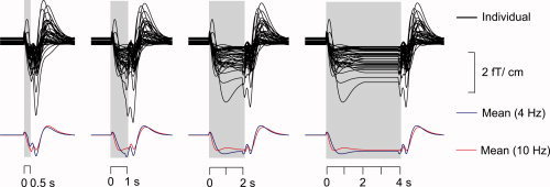
Predictions for all 40 individual conditions (10 subjects, two hemispheres, and two stimulus repetition rates) using the linear bivariate model separately for all block durations (0.5, 1, 2, and 4 s) (above). Mean predictions across the 20 conditions (10 subjects, two hemispheres), separately for the 4‐Hz and 10‐Hz repetition rates (below).

Model Diagnostics

Figure 6 shows the observed signals and the predicted outputs (from linear bivariate, nonlinear bivariate, and univariate models) for the right rolandic signal of subject S3 stimulated with 4‐Hz trains. The typical suppression‐rebound response is well predicted by all three models, and the onset response appropriately predicts only the suppression. The univariate model (bottom panels) does not properly predict the responses for short durations (0.5 and 1 s). For the linear bivariate model (top panels), the offset response alone predicts the rebound. However, it also suggests a post‐offset dip that is not seen in the data. A similar post‐offset dip is present to a lesser extent in the nonlinear bivariate model output (middle panels), because the rebound is predicted together by the offset and interaction response. However, this improvement comes at the cost of six additional model parameters. Table I lists the mean values of the parameters across all subjects, for the univariate, the linear bivariate and nonlinear bivariate models, and the correlation coefficients. The mean correlation coefficient for the boxcar predictor was 0.44 ± 0.02. All three models improved upon this value, the linear bivariate by 43%, the nonlinear bivariate by 25%, and the univariate by 32% (see Table I). Given that the linear bivariate model is a better fit and more parsimonious than the nonlinear model, we considered it sufficient to validate this model alone on the test dataset.

Figure 6.

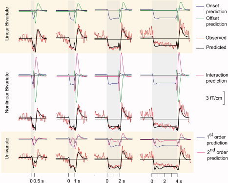
The observed and predicted 20‐Hz envelopes for all stimulus durations (4‐Hz stimulus rate) for a representative subject (S3) for the linear bivariate model (top panel), the nonlinear bivariate model (middle panel), and the univariate model (lower panel). For the linear bivariate model, the entire envelope was modeled using an onset response and an offset response, obtained by convolution of the stimulus time course with the onset kernel and the offset “impulse function” with the offset kernel. In the nonlinear bivariate model, an additional second‐order interaction kernel was used. In the univariate model, there was no partitioning into onset and offset response; the univariate first‐ and second‐order kernels operated directly on the stimulus time course.

Table I.

The group‐mean parameters of the linear bivariate, the nonlinear bivariate and the univariate models

	Linear	Bivariate	Nonlinear	Bivariate	Univariate		Boxcar
β	c 0	0.1056	c 0	0.1245	c 0	0.0947
	c 1(1)	0.0662	c 1(1)	0.0718	c 1(1)	0.0537
	c 1(2)	0.0359	c 1(2)	0.0567	c 1(2)	0.0169	—
	c 1(3)	0.0076	c 1(3)	0.0196	c 1(3)	0.0022
	c 2(1)	0.0664	c 2(1)	0.2075	c 2(1,1)	−0.0018
	c 2(2)	0.0941	c 2(2)	−0.0698	c 2(1,2)	−0.0066
	c 2(3)	−0.0300	c 2(3)	−0.0960	c 2(1,3)	−0.0031	–
			c 3(1,1)	0.0683	c 2(2,2)	−0.0115
			c 3(1,2)	−0.0501	c 2(2,3)	−0.0140
			c 3(1,3)	0.0336	c 2(3,3)	−0.0044
			c 3(2,2)	0.0163
			c 3(2,3)	0.0031
			c 3(3,3)	0.0071
α		0.8117		0.8104		0.8012
CC		0.63 (0.03)		0.55 (0.03)		0.58 (0.02)	0.44 (0.02)

These include the coefficients for the kernels, β, and the Laguerre pole, α. The mean correlation coefficient (CC) obtained from the cross‐validation approach (see text) is also shown for each model, including the stimulus time course (boxcar). The standard errors of mean (SEMs) for the correlation coefficient are shown in parenthesis.

Characteristics of Convolution Kernels

The univariate model

Supporting Information Figure S2 shows the first‐ and second‐order kernels for the univariate model. The first‐order kernel predicts the response to an input of infinitesimal duration, in this case a brief bilateral tactile pulse. The second‐order kernels are two‐dimensional functions of time. They may be interpreted as the response to a pair of unit impulses applied in quick succession. Specifically, k ₂(t ₁, t ₂) predicts the response at time t ₁ to a pair of impulses δ(t) and δ(t − t ₂).

The bivariate model

Figure 7 shows the onset, offset, and interaction kernels for the nonlinear bivariate model computed from the group‐mean parameters. The onset and offset kernels for the linear bivariate model were similar (not shown). The onset and offset kernels may be interpreted as together predicting the linear part of the response to a stimulus of infinitesimal duration. A straightforward interpretation of the interaction kernel is through its projections, as illustrated in Figure 7c. A slice of the two‐dimensional kernel along the axis τ₁ − τ₂ = Δ describes the effect of interaction between the onset and offset events, occurring at an event separation of Δ, i.e. for a stimulus of duration Δ. The relationship of kernel morphology to physiology is unclear, particularly so for the offset and interaction kernels.

Figure 7.

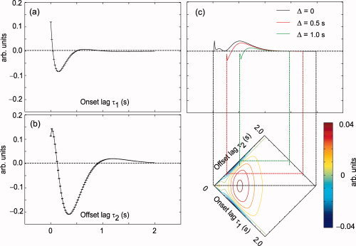
Onset (a), offset (b), and interaction (c) kernels of the bivariate nonlinear model. The kernels were computed from the mean set of parameters across subjects and conditions. Slices of the interaction kernel parallel to the diagonal represent the nonlinear component of the predicted response, at respective time separations between onset and offset i.e. stimulus durations. Slices corresponding to durations 0, 0.5, and 1.0 s are shown.

Model Validation

Figure 8 (left panel) shows, on the Free Surfer Average (FSA) brain, the modulation depth maps (MDMs) as predicted by the stimulus time course (boxcar) and the linear bivariate model. The predictions were confined to the hand area of the primary motor cortex (MI), which is the most plausible generator site of the 20‐Hz component of the mu rhythm in our experimental setup.

Figure 8.

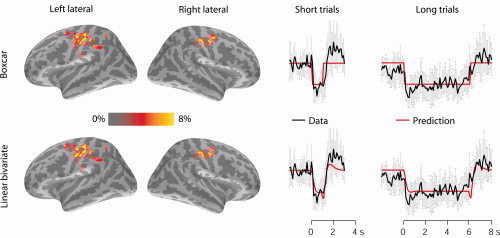
Predictions of spatial generators of the 20‐Hz rhythm, and the corresponding time courses. Left: The mean modulation depth maps (MDMs) across subjects, resulting from a general linear model (GLM) of the cortical current envelopes, with the boxcar, and the linear bivariate model separately used as regressors. All MDMs were projected on an inflated Free Surfer Average (FSA) brain. The colored regions represent the source points with top 1% modulation depth. Right: The mean envelopes of the cortical minimum‐norm estimates for the source point with maximum MD, further averaged across the test subjects for both short (1‐s) and long (6‐s) stimulus blocks. Predictions of the envelope by the stimulus time course (top) and the linear bivariate model (bottom), are overlaid on the envelopes. The models were derived from the training data. The error bars show standard errors of mean (N = 5 subjects).

For each test subject, Figure 8 (right panel) shows the averages of the estimated cortical envelopes (for the 1‐s and 6‐s stimulus blocks), as well as their predictions by the stimulus time course and by the linear bivariate model. These averages at the source point showing the maximum modulation depth were further averaged across the test subjects. Note that the applied ORF model is the average model based on the training dataset, not optimized for test subjects, stimulus rate or duration.

In addition to the shape of the envelope predicted by the model, the “baseline” level of rhythmic activity is known to vary across subjects. Such variability was observed in the “baseline” levels of the envelopes estimated from the GLMs (Supporting Information Fig. S3). For long‐duration blocks, the cortical envelopes do not stay suppressed at a constant level below the “baseline” level; rather they may briefly return to the baseline during the stimulation.

Table II lists the maximum MDs within the sensorimotor cortex for each subject, in each hemisphere, and the correlation coefficients between estimated and predicted envelopes for both 1‐s and 6‐s stimulus blocks. The left‐ and right‐hemisphere data show no consistent differences. The correlation coefficients show that the ORF model predicts the envelope dynamics for the 1‐s stimulus block 20% (P = 0.038) more effectively than the stimulus time course.

Table II.

The subjectwise maximum modulation depths (MaxMD) in the rolandic region for each hemisphere of the test subjects, and the correlation coefficients between predicted and estimated cortical responses

Subject	Linear bivariate		Correlation		Boxcar		Correlation
	MaxMD(L)	MaxMD(R)	1 s	6 s	MaxMD(L)	MaxMD(R)	1 s	6 s
S2	24	12	0.73	0.59	22	12	0.53	0.52
S11	12	16	0.64	0.59	11	17	0.57	0.61
S12	16	8	0.53	0.44	15	7	0.46	0.46
S13	20	16	0.72	0.55	20	15	0.57	0.63
S14	28	28	0.69	0.74	26	28	0.62	0.71
Mean SD	20.0 ± 6.3	16.0 ± 7.5	0.66 ± 0.08	0.58 ± 0.11	18.8 ± 5.9	15.8 ± 7.8	0.55 ± 0.06	0.59 ± 0.10
MNM	12	10			12	9

Both the mean (± standard‐deviation, SD) of the single subject maxima, and the mean of the maxima (MNM) after normalization to the Free Surfer Average (FSA) brain are given. The means (± SD) for the correlation coefficients are also listed.

DISCUSSION

We introduced a quantitative model—based on a generalized convolution approach—for the dynamics of event‐related rhythmic MEG activity. Univariate and bivariate generalized convolution models were fit to the 20‐Hz envelope of the mu rhythm at representative channels. The models were estimated with a supervised machine‐learning approach. The temporal characteristics of the convolution kernels of all models were consistent across subjects and conditions. The generalizability of the models was tested using a different experimental paradigm and a validation approach based on mapping of GLM coefficients on to the cortical surface; the models generalized across subjects, stimulus paradigms, and analysis methods, i.e. from event‐related averages to unaveraged envelopes and from sensor to source space. However, it is important to emphasize that this approach represents only a first step towards generalization, and further studies are needed to quantify the dependence of the model on stimulus parameters.

For the first time with MEG data, we introduced a general linear model approach (conventionally applied to fMRI analysis of block‐design experiments) to make inferences on unaveraged cortical current envelopes by visualizing their modulation depths over the entire cortical surface. Statistically significant local maxima in the primary motor cortex were related to the rolandic 20‐Hz rhythms, lending credibility to the models' ability to predict cortical generators of oscillatory responses.

On the Model Structure

The expansion order of the Volterra series and the number of basis functions used to model the Volterra kernels are the two key determinants of the model structure.

Truncation of the Volterra series to the second order is practical and does not pose a serious problem for the following reasons. First, the number of parameters required for the model grows exponentially with the order. To prevent overlearning (a phenomenon showing an excellent fit to the training set but poor test set generalization), we need exponentially more data to estimate the model. Some symptoms of overlearning were already observable in the cross‐validation, based on within‐training‐set predictive power, where the linear bivariate model with eight parameters outperformed the nonlinear bivariate model with 14 parameters. Increasing the number of parameters is likely to result in poorer generalization. Second, if the 2‐s kernel support is a reasonable assumption, the second‐order kernel appears sufficient to represent this nonlinearity. Last, higher‐order kernels are extremely hard to interpret. In the literature on applications of Volterra theory cited here, higher‐order terms were not used.

The number of basis functions must be large enough to capture the essential temporal features of the envelope dynamics. Simultaneously, it must be small enough so that the least‐squares estimation is numerically well‐posed, and also minimize overfitting the nonessential features of the envelope.

The correlation coefficients, used as measures of prediction performance, showed that for the training dataset the linear bivariate model performed significantly better than the nonlinear bivariate model and equally as well as the univariate model. Further, the linear bivariate model, specified by eight parameters, is more parsimonious than both the nonlinear bivariate and the univariate models which require 14 and 11 parameters, respectively. One concern for future applications of this model is the tradeoff between predictive accuracy (benefit provided by an accurate fit) and model complexity (the cost incurred in applying it) relative to the boxcar. Therefore, further research is required to come up with objective measures of integrating fit and complexity. For instance, Bayesian model selection techniques, such as those applied in the dynamic causal modeling (DCM) framework [Penny et al., 2004], may be explored.

Since the two inputs to the bivariate model are not independent, it may be rewritten as a univariate model with two kernels:

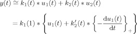(12)

where, k ₁(t) * k ₂′(t) = k ₂(t). This model could be interpreted as a linear transformation of the boxcar input, with a suitable nonlinearity added at the stimulus offset alone. The nonlinearity in this case would be a rectified version of the negative time derivative of the stimulus time course. Such a model may be viewed alongside a class of linearized models for predicting the hemodynamic response in fMRI, in which the stimulus time course is first, prior to convolution with the HRF, transformed at the onset to account for neural adaptation effects [Nangini et al., 2005; Soltysik et al., 2004].

Interpretation of Model Parameters

The averaging of model parameters across stimulus conditions deserves careful attention. Since only one among the eight parameters differed significantly between the 10‐ and 4‐Hz conditions, and this single parameter only for the linear bivariate model, we averaged the parameters across all conditions without doing an explicit sensitivity analysis to determine the significance of each parameter. The goals of a maximally generalizable and a maximally discriminative model are contradictory. In this work, we opted for the former. Further research involving carefully designed stimulus sequences is required to build more discriminative models.

Although the model allowed to predict the spatial distribution of rhythmic activity represented by cortical minimum‐norm estimates, the parameters themselves are not informative about the physiological mechanisms underlying modulations of the brain rhythms. Conversely, the generalized convolution framework is convenient in the sense that no assumptions are required about the generative process (provided that the span of the basis functions used, in this case the Laguerre polynomials, is sufficiently comprehensive) that gives rise to the modulations. In this sense, the empirical, black‐box model is more flexible in modeling the true characteristics of the response than, for instance, a neural mass model of rhythmic activity [Jansen and Rit, 1995] derived from elementary building blocks. This important distinction between black‐box models and generative models was well emphasized by Friston et al. [ 2000] who compared their empirical, nonlinear Volterra model of the hemodynamic response [Friston et al., 1998] with the balloon model [Buxton et al., 1998], a mechanistic model of the hemodynamic response with physiologically meaningful parameters. The Volterra kernels corresponding to the balloon model resembled the empirically derived kernels, and the empirically derived kernels in turn were explained by physically plausible balloon model parameters.

Drawing on these lines, it would be instructive to study the properties of the ORF convolution kernels associated with generative models of neural dynamics, such as the neural mass model. Such a study could potentially both motivate the ORF physiologically and demonstrate the adequacy of the generative model for predicting the response. In this context, studies by Valdes et al. [ 1999] and Sotero et al. [ 2007] are particularly noteworthy, since they both applied generative models for explaining observed EEG data. Valdes et al. [ 1999] fit the parameters of the neural mass model of Zetterberg et al. [ 1978] to real EEG data within a maximum likelihood framework. Sotero et al. [ 2007] extended the model by David and Friston [ 2003] to build generative models of several EEG/MEG rhythms; the models were able to explain temporal, spatial, and spectral characteristics of alpha, beta, gamma, delta, and theta rhythms. The model was also able to predict the suppression of alpha activity resulting from simulated visual input applied at the thalamic level.

Model Generalization

For the test set, the model was a significantly more effective predictor than the stimulus time course for the short but not for the long stimulus blocks. At least two reasons may account for this observation. First, the model was not trained on 6‐s but 1‐s blocks. Second, as the stimulus prolongs, the suppression part of the response dominates. Since an inverted stimulus time course captures the suppression well, the rebound‐related nonlinearity not captured by the boxcar contributes less to the model error, and hence to the correlation coefficient.

The baseline level of the cortical rhythms varies according to the subject, and this variation is well reflected in the GLM coefficients. Additionally, in our subjects, the suppression of the cortical rhythms did not stay constant during the long‐duration stimuli in the test set, but the level fluctuated considerably. Such fluctuations were variable across the five test subjects, and were not predicted by the model.

We advocate the framework as a broad, quantitative approach to characterize oscillatory dynamics of brain rhythms with specific temporal, spectral, and spatial characteristics. However, it is important to clarify that the generalizability of the model does not imply that a single ORF can model all kinds of brain rhythms, such as induced alpha or gamma oscillations. The parameters of the model have to be uniquely derived for each type of brain rhythm.

Thus, although the ORF model may not be optimally generalizable, its parametric nature makes it sufficiently generalizable to discriminate between conditions of interest. An analogous situation is frequently encountered in the fMRI literature where a simple, linear hemodynamic response function works well as a general discriminative model, although it is widely agreed that the true hemodynamic response is a complex, nonlinear phenomenon that varies across brain areas and subject groups [Handwerker et al., 2004].

Potential Applications of the Model

Although our goal was to obtain a general model of the dynamics of rhythmic activity, quantitative models, such as the ORF, may be used to systematically explore the effects of stimulus parameters, such as intensity, duration, and adaptation, as well as of disease and age, by capturing their effects in a few parameters. The parameters may prove a useful tool to reliably discriminate between different tasks and pathologies, as well as to characterize intersubject differences. To study the variation of the dynamics of a rhythm as a function of cortical location, the ORF model could be extended so that it is separately optimized for each cortical source point.

Task‐specific effects on the rhythms could also be studied using the GLM approach to MEG data, especially in source space. A challenging and interesting application of this approach is in the analysis of brain imaging data from different methods where direct comparisons are sought between fast electrical fluctuations, measured by EEG or MEG, and slow hemodynamics, measured by fMRI. Another interesting application of the ORF/GLM approach is to map the cortical generators of the suppression and the rebound separately, using the onset and offset predictions of the linear bivariate model simultaneously as GLM regressors.

The generalized convolution approach is sufficiently broad in the sense that the same framework may be applied to study dynamics of neural activity at various scales, from single‐unit electrophysiological recordings to noninvasive methods such as MEG. For these reasons, it seems feasible and worthwhile to quantitatively model the dynamics of the brain's electromagnetic rhythmic activity.

Supporting information

Additional Supporting Information may be found in the online version of this article.

Supplemental Figure1.

Supplemental Figure2.

Supplemental Figure3.

REFERENCES

- Back AD,Tsoi AC ( 1996): Nonlinear system identification using discrete Laguerre functions. J Sys Eng 6: 194–207. [Google Scholar]
- Broome PW ( 1965): Discrete orthonormal sequences. J Assoc Comput Mach 12: 151–168 [Google Scholar]
- Buxton RB,Wong EC,Frank LR ( 1998): Dynamics of blood flow and oxygenation changes during brain activation: the balloon model. Magn Reson Med 39: 855–864. [DOI] [PubMed] [Google Scholar]
- Campello RJGB,Favier G,Wagner C ( 2004): Optimal expansions of discrete‐time Volterra models using Laguerre functions. Automatica 40: 815–822. [Google Scholar]
- Dale AM ( 1999): Optimal experimental design for event‐related fMRI. Hum Brain Mapp 8: 109–114. [DOI] [PMC free article] [PubMed] [Google Scholar]
- Dale AM,Liu AK,Fischl BR,Buckner RL,Belliveau JW,Lewine JD,Halgren E ( 2000): Dynamic statistical parametric mapping: Combining fMRI and MEG for high‐resolution imaging of cortical activity. Neuron 26: 55–67. [DOI] [PubMed] [Google Scholar]
- David O,Friston KJ ( 2003): A neural mass model for MEG/EEG: Coupling and neuronal dynamics. Neuroimage 20: 1743–1755. [DOI] [PubMed] [Google Scholar]
- Friston KJ,Josephs O,Rees G,Turner R ( 1998): Nonlinear event‐related responses in fMRI. Magn Reson Med 39: 41–52. [DOI] [PubMed] [Google Scholar]
- Friston KJ,Mechelli A,Turner R,Price CJ ( 2000): Nonlinear responses in fMRI: The Balloon model, Volterra kernels, and other hemodynamics. Neuroimage 12: 466–477. [DOI] [PubMed] [Google Scholar]
- Handwerker DA,Ollinger JM,D'Esposito M ( 2004): Variation of BOLD hemodynamic responses across subjects and brain regions and their effects on statistical analyses. NeuroImage 21: 1639–1651. [DOI] [PubMed] [Google Scholar]
- Hari R,Forss N,Avikainen S,Kirveskari E,Salenius S,Rizzolatti G ( 1998): Activation of human primary motor cortex during action observation: A neuromagnetic study. Proc Natl Acad Sci USA 95: 15061–15065. [DOI] [PMC free article] [PubMed] [Google Scholar]
- Huettel SA,Obembe OO,Song AW,Woldorff MG ( 2004): The BOLD fMRI refractory effect is specific to stimulus attributes: Evidence from a visual motion paradigm. Neuroimage 23: 402–408. [DOI] [PubMed] [Google Scholar]
- Jansen BH,Rit VG ( 1995): Electroencephalogram and visual evoked potential generation in a mathematical model of coupled cortical columns. Biol Cybern 73: 357–366. [DOI] [PubMed] [Google Scholar]
- Jones SR,Pritchett DL,Stufflebeam SM,Hämäläinen MS,Moore CI ( 2007a): Neural correlates of tactile detection: A combined magnetoencephalography and biophysically based computational modeling study. J Neurosci 27: 10751–10764. [DOI] [PMC free article] [PubMed] [Google Scholar]
- Jones SR,Pritchett DL,Stufflebeam SM,Hämäläinen MS,Moore CI ( 2007b): Pre‐stimulus somatosensory μ‐rhythms predict perception: A combined MEG and modeling study. Society for Neuroscience abstracts archive. Soc Neurosci Ann Meeting, San Diego. Also available at: www.sfn.org.
- Krusienski DJ,Schalk G,McFarland DJ,Wolpaw JR ( 2007): A μ‐rhythm matched filter for continuous control of a brain‐computer interface. IEEE Trans Biomed Eng 54: 273–280. [DOI] [PubMed] [Google Scholar]
- Lee S‐K,Yoon HW,Chung J‐Y,Song M‐S,Park H ( 2004): Analysis of functional MRI data based on an estimation of the hemodynamic response in the human brain. J Neurosci Meth 139: 91–98. [DOI] [PubMed] [Google Scholar]
- Lin F‐H,Belliveau JW,Dale AM,Hämäläinen MS ( 2006): Distributed current estimates using cortical orientation constraints. Hum Brain Mapp 27: 1–13. [DOI] [PMC free article] [PubMed] [Google Scholar]
- Lopes da Silva FH,Hoeks A,Smits H,Zetterberg LH ( 1974): Model of brain rhythmic activity. Biol Cybern 15: 27–37. [DOI] [PubMed] [Google Scholar]
- Mantini D,Perrucci MG,Gratta CD,Romani GL,Corbetta M ( 2007): Electrophysiological signatures of resting state networks in the human brain. Proc Natl Acad Sci USA 104: 13170–13175. [DOI] [PMC free article] [PubMed] [Google Scholar]
- Marmarelis VZ ( 1993): Identification of nonlinear biological systems using Laguerre expansions of kernels. Ann Biomed Eng 21: 573–589. [DOI] [PubMed] [Google Scholar]
- Nangini C,Macintosh BJ,Tam F,Staines WR,Graham SJ ( 2005): Assessing linear time‐invariance in human primary somatosensory cortex with BOLD fMRI using vibrotactile stimuli. Magn Reson Med 53: 304–311. [DOI] [PubMed] [Google Scholar]
- Penny WD,Stephan KE,Mechelli A,Friston KJ ( 2004): Comparing dynamic causal models. Neuroimage 22: 1157–1172. [DOI] [PubMed] [Google Scholar]
- Ritter P,Moosmann M,Villringer A ( 2009): Rolandic alpha and beta EEG rhythms' strengths are inversely related to fMRI‐BOLD signal in primary somatosensory and motor cortex. Hum Brain Mapp 30: 1168–1187. [DOI] [PMC free article] [PubMed] [Google Scholar]
- Salmelin R,Hari R ( 1994): Spatiotemporal characteristics of sensorimotor neuromagnetic rhythms related to thumb movement. Neurosci 60: 537–550. [DOI] [PubMed] [Google Scholar]
- Salmelin R,Hämäläinen M,Kajola M,Hari R ( 1995): Functional segregation of movement‐related rhythmic activity in the human brain. Neuroimage 2: 237–243. [DOI] [PubMed] [Google Scholar]
- Schetzen M ( 2006): The Volterra and Wiener Theories of Nonlinear Systems. Revised ed. Malabar, Florida: Krieger Publishing Company; 618 p. [Google Scholar]
- Schnitzler A,Salenius S,Salmelin R,Jousmäki V,Hari R ( 1997): Involvement of primary motor cortex in motor imagery: A neuromagnetic study. Neuroimage 6: 201–208. [DOI] [PubMed] [Google Scholar]
- Soltysik DA,Peck KK,White KD,Crosson B,Briggs RW ( 2004): Comparison of hemodynamic response nonlinearity across primary cortical areas. Neuroimage 22: 1117–1127. [DOI] [PubMed] [Google Scholar]
- Sotero RC,Trujillo‐Barreto NJ,Iturria‐Medina Y,Carbonell F,Jimenez JC ( 2007): Realistically coupled neural mass models can generate EEG rhythms. Neural Computat 19: 478–512. [DOI] [PubMed] [Google Scholar]
- Taulu S,Kajola M ( 2005): Presentation of electromagnetic multichannel data: The signal space separation method. J App Phys 97: 124905–124910. [Google Scholar]
- Taulu S,Simola J ( 2006): Spatiotemporal signal space separation method for rejecting nearby interference in MEG measurements. Phys Med Biol 51: 1759–1768. [DOI] [PubMed] [Google Scholar]
- Valdes PA,Jimenez JC,Riera J,Biscay R,Ozaki T ( 1999): Nonlinear EEG analysis based on a neural mass model. Biol Cybern 81: 415–424. [DOI] [PubMed] [Google Scholar]
- Victor JD ( 2005): Analyzing receptive fields, classification images and functional images: Challenges with opportunities for synergy. Nat Neurosci 8: 1651–1656. [DOI] [PMC free article] [PubMed] [Google Scholar]
- Watanabe A,Stark L ( 1975): Kernel method for nonlinear analysis: Identification of a biological control system. Math Biosci 27: 99–108. [Google Scholar]
- Wiener N. 1958. Nonlinear Problems in Random Theory, 1st ed. Cambridge, Massachusetts: MIT Press; 144 p. [Google Scholar]
- Zetterberg LH,Kristiansson L,Mossberg K ( 1978): Performance of a model for a local neuron population. Biol Cybern 31: 15–26. [DOI] [PubMed] [Google Scholar]
Associated Data
This section collects any data citations, data availability statements, or supplementary materials included in this article.
Supplementary Materials