Using the wild bootstrap to quantify uncertainty in diffusion tensor imaging

Abstract

Estimation of noise‐induced variability in diffusion tensor imaging (DTI) is needed to objectively follow disease progression in therapeutic monitoring and to provide consistent readouts of pathophysiology. The noise variability of nonlinear quantities of the diffusion tensor (e.g., fractional anisotropy, fiber orientation, etc.) have been quantified using the bootstrap, in which the data are resampled from the experimental averages, yet this approach is only applicable to DTI scans that contain multiple averages from the same sampling direction. It has been shown that DTI acquisitions with a modest to large number of directions, in which each direction is only sampled once, outperform the multiple averages approach. These acquisitions resist the traditional (regular) bootstrap analysis though. In contrast to the regular bootstrap, the wild bootstrap method can be applied to such protocols in which there is only one observation per direction. Here, we compare and contrast the wild bootstrap with the regular bootstrap using Monte Carlo numerical simulations for a number of diffusion scenarios. The regular and wild bootstrap methods are applied to human DTI data and empirical distributions are obtained for fractional anisotropy and the diffusion tensor eigensystem. Spatial maps of the estimated variability in the diffusion tensor principal eigenvector are provided. The wild bootstrap method can provide empirical distributions for tensor‐derived quantities, such as fractional anisotropy and principal eigenvector direction, even when the exact distributions are not easily derived. Hum Brain Mapp, 2008. © 2007 Wiley‐Liss, Inc.

INTRODUCTION

Regardless of the sampling scheme used, it is important to properly characterize the amount of uncertainty in derived quantities from the estimated diffusion tensor. For quantities of interest based on linear combinations of elements in the diffusion tensor, such as mean diffusivity, one can quantify variability through confidence intervals derived from the noise properties of magnitude images and the theory of linear models [Salvador et al., 2005]. However, quantities based on nonlinear combinations of elements from the diffusion tensor (e.g., eigenvalues, eigenvectors, fractional anisotropy, etc.) are not easily obtained analytically1 and computational methods are utilized instead. When a relatively low number of gradient directions are sampled, it is common to obtain multiple measurements in each direction during the scanning session. If this is the case, then the bootstrap [Efron, 1981; Efron and Tibshirani, 1993] has been used to help quantify uncertainty in scalar summaries of DTI [Heim et al., 2004; Jones, 2003; Pajevic and Basser, 2003]. Uncertainty in the diffusion tensor is also very important for tractography [Behrens et al., 2003] and the bootstrap has already been successfully applied [Jones and Pierpaoli, 2005; Jones et al., 2005].

The bootstrap method, as previously implemented in DTI, requires multiple observations per gradient direction in order to perform the resampling. With sampling schemes acquiring a large number of directions being used more and more in a clinical setting [Jones, 2004; Jones et al., 1999a], it is becoming less likely that more than one measurement per gradient direction is obtained—excluding the application of this particular implementation of the bootstrap (we call this the regular bootstrap from now on). An investigation into how many repeat acquisitions are required to gain accurate results from the regular bootstrap concluded that no benefit in accuracy or precision was gained by using more than seven repeat acquisitions and fewer than four repeat acquisitions resulted in poor precision with significant errors [O'Gorman and Jones, 2005]. For example, with a whole‐brain acquisition protocol taking 10–15 min to acquire a single volume, it would be difficult to push the number of repeat acquisitions tolerated by patients with mild disorders beyond three or four. Being able to apply resampling procedures to either (a) fewer repeat acquisitions or (b) acquisitions with a relatively high number of gradient directions with no repeated measurements without losing the ability to characterize the intrinsic variability of statistical summaries of DTI is highly desirable.

We introduce model‐based resampling techniques [Davison and Hinkley, 1997], in particular, the wild bootstrap [Flachaire, 2005; Liu, 1988], that may be applied to the residuals from the multiple linear regression model used to estimate elements of the diffusion tensor at each voxel. The wild bootstrap is specifically designed to work when the model is heteroscedastic; that is, when the variance of the errors is not constant for all observations. In the case of DTI, this corresponds to the assumption of nonconstant variance for the log‐transformed NMR signal [Basser et al., 1994; Salvador et al., 2005]. The relationship between noise and b‐value and their influence on quantities derived from the diffusion tensor, such as fractional anisotropy, was recently described in Jones and Basser [2004]. A simple modification to the basic model‐based bootstrap allows this methodology to be applied when multiple measurements are acquired in each gradient direction. Thus, the model‐based bootstrap techniques presented here may be applied to both research and clinical DTI protocols assuming that more than six gradient directions have been acquired or that a six‐direction gradient encoding scheme has been acquired more than once.

Statistical methods, such as the bootstrap, are not the only way to quantify uncertainty in DTI. There are numerous references based on analytical techniques, such as “propagation of errors”. First and second‐order corrections to the eigenvalues and eigenvectors from perturbation theory were used to correct for noise distortions in Anderson [2001]. Measures of anisotropy, obtained without diagonalizing the tensor, were studied using propagation of errors to compare sampling schemes in Poonawalla and Zhou [2004]. Numerical methods, such as Monte Carlo simulation, have also been used to investigate the effect of noise on quantitative measurements of anisotropy especially those based on eigenvalues (i.e., the sorting bias) [Batchelor et al., 2003; Pierpaoli and Basser, 1996; Skare et al., 2000].

This study investigates the ability of model‐based resampling, in particular, the wild bootstrap, to provide reasonable estimates of variability for derived quantities of the diffusion tensor when one or more measurements per gradient direction are available. Two sampling schemes, six directions and 60 directions, are used to produce both simulated and clinical DTI data. Comparisons are made for regular and wild bootstrap estimates of variability on the eigenvalues, fractional anisotropy, and fiber orientation derived from the diffusion tensor. With standard errors based on the bootstrap now available for all image acquisition schemes, it is hoped that reporting both parameter estimates and standard errors for summaries of anisotropy will become more widespread.

THEORY

The regular bootstrap is a general statistical technique where an observed set of measurements is sampled with replacement over‐and‐over again in order to characterize a statistic of interest [Davison and Hinkley, 1997; Efron and Tibshirani, 1993]. The regular bootstrap places equal probability on independent observations when resampling, and is therefore only appropriate when more than one measurement per direction is available (although this is not strictly true, a point which we move onto later). This framework is common in DTI scans when the acquisition sequence contains relatively few gradient directions (e.g., six) but becomes less clinically feasible as the number of gradient directions increases. Further details and examples concerning the implementation of the regular bootstrap in DTI data analysis may be found in Pajevic and Basser [2003] and Heim et al. [2004].

Although six gradient directions are the minimum number to estimate the unique elements of the diffusion tensor, there are numerous sampling schemes that have been recommended with many more gradient directions [Batchelor et al., 2003; Hasan and Narayana, 2003; Jones et al., 1999a, b] or it is common practice to obtain several measurements in each direction when a relatively low number of gradient directions are sampled. Because of the constraints in a clinical setting there are relatively few DTI scans with a large number of directions and repeated measurements. Hence, obtaining estimates of standard errors for scalar quantities of interest based on the diffusion tensor are not available using the regular bootstrap. This leads us to consider alternative bootstrap methodology that operates within the log‐linear relationship between echo attenuation and the diffusion model.

Model‐Based Resampling: Homoscedastic Errors

First, we describe the theory around the model‐based resampling of errors in a linear regression model and then introduce the wild bootstrap. Model‐based resampling in linear regression is a popular nonparametric technique to infer properties of the parameter estimates from the linear model. Let us assume that the standard model for signal intensity in DTI is given by S (x _i) = S ₀ exp (− b x ${}_{\mathit{\text{i}}}^{\mathit{\text{T}}}$ D x _i), where D is the diffusion tensor, x _i = (x _i1, x _i2, x _i3)^T is the gradient direction for the ith observation (i = 1,…,N) and b is the diffusion weighting. Applying the log transform to both sides allows us to use notation for a multiple linear regression model [Basser et al., 1994]

(1)

to estimate the diffusion tensor from observed data. In Eq. (1) y is a length N vector of the log‐transformed signal intensities, X is a N × 7 direction matrix

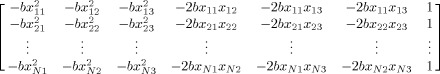(2)

d = [D _xx D _yy D _zz D _xy D _xz D _yz log(S ₀)]^T and ε is a length N vector of errors. The ordinary least‐squares (OLS) estimate of d is given by d̂ = (X^T X)⁻¹ X^T y. After the initial OLS operation, a weighting matrix W may be calculated via

(3)

where I _N is the N × N identity matrix. The weighted least‐squares (WLS) estimate of d is then given by d̂=(X^T W ⁻² X)⁻¹ X^T W ⁻² y [Salvador et al., 2005]. This implementation of WLS is similar to the approach found in Basser et al. [1994], the difference being that fitted values from the least‐squares regression are used instead of the observations in constructing the weighting matrix W.

The assumptions we make on the structure of ϶ determine which bootstrap method is appropriate. Under the assumption that ϶ is a vector of independent and identically distributed (IID) random variables with zero mean, the linear regression would be termed homoscedastic and we would be able to randomly sample with replacement from the errors. Model‐based resampling of the errors would take the form

(4)

where (X d)_i is the product of the ith row of X and d, and ε${}_{\mathit{\text{i}}}^{\text{★}}$ is a random sample from the residuals of the original regression model. Performing WLS on y ^★ will produce a model‐based bootstrap estimate of the tensor d ^★. Repeating these steps, resampling and estimation, builds up a collection of tensors called a (model‐based) bootstrap distribution. Summary statistics from this empirical distribution can be used to describe the original parameter estimate.

Model‐Based Resampling: Heteroscedastic Errors

The assumption of homoscedasticity is not valid for DTI when a linear regression model is used to estimate the diffusion tensor. This violation is induced by applying the logarithmic transform in order to achieve the linear relationship in Eq. (1) and is overcome through the use of WLS regression, as originally noted in Basser et al. [1994]. When the assumption of IID errors is not valid, the regression model is termed heteroscedastic. When a relatively small number of gradient directions are used to acquire the data, a simple modification to the basic model‐based bootstrap procedure can adapt to the situation where multiple measurements per direction are available. We call this technique “resampling within gradient directions” (RWGD). Rewrite the vector of observations (log‐transformed signal intensities) as being indexed by gradient directions and measurements per direction

(5)

in this specific case y ₀ denotes the b = 0 acquisitions and y ₁,…,y ₆ denote the acquisitions corresponding to six gradient directions. For convenience, assume that the rows of X may be indexed the same way. The RWGD bootstrap sample would take the form

(6)

so that each subvector y_j conforms with Eq. (4), thus ensuring that all resampling is kept within each gradient direction.

The wild bootstrap [Liu, 1988] is a method for model‐based resampling in heteroscedastic linear regression with an unknown form; i.e., when the errors have an arbitrary variance structure. Model‐based resampling, using the wild bootstrap, is given by

(7)

where a _i is a weight in order to produce a heteroscedasticity consistent covariance matrix estimator (HCCME), u _i is the residual and ε${}_{\mathit{\text{i}}}^{\text{★}}$ is drawn from the distribution F. The HCCME is required because a standard assumption of linear regression models—the error terms have a constant variance—is violated here [MacKinnon and White, 1985]. Instead of resampling from the residuals of the linear regression, only valid in the homoscedastic case, the wild bootstrap samples from an auxiliary distribution F and multiplies this random variable with a rescaled version of the residual a _i u _i using a local estimate of the covariance matrix. Examples of such HCCMEs include

(8)

where n is the total number of observations, p is the number of estimated parameters, and h _i is the ith diagonal element from H=X(X ^T X)⁻¹ X ^T, the so‐called hat matrix from OLS regression. Detailed explanations of the HCCMEs are beyond the scope of this study and can be found in MacKinnon and White [1985]. Briefly, the first form in Eq. (8) comes from a degrees of freedom correction and the second and third forms can be derived from jackknife‐based estimators of the covariance matrix. The bootstrap performance between the different versions is discussed in Flachaire [2005] and results from DTI‐specific simulations are provided in this article.

The random variable ϵ ^★ obtained from the auxiliary distribution must satisfy

(9)

(10)

that is, its first moment is zero and its second moment is one, to ensure that the residual from the wild bootstrap in Eq. (7) retains the same first and second moments as the true residual. An additional condition

(11)

its third moment is one, is commonly added to help define this distribution. It has been shown, assuming Eqs. (9), (10), (11), that the first three moments of the bootstrap distribution of an HCCME‐based test statistic agree with those from the true distribution of the statistic up to order n ⁻¹ [Liu, 1988]. Two suggestions for the auxiliary distribution F are

(12)

[Mammen, 1993] and the Rademacher distribution

(13)

[Davidson and Flachaire, 2001; Liu, 1988]. Simulation studies in Davidson and Flachaire [2001] have indicated that the wild bootstrap using F ₂ outperforms the wild bootstrap using F ₁, especially when the errors follow a skewed distribution. Additional proposals for auxiliary distributions may be found in Liu [1988] and Mammen [1993].

Note the residuals are no longer resampled in Eq. (7) to generate the wild bootstrap sample, unlike the ordinary model‐based bootstrap sample in Eq. (4). This respects the heteroscedasticity in the model but still produces enough variability to draw inference about the parameters (diffusion tensor elements) in the multiple linear regression model. An example of the wild bootstrap applied to a single voxel, taken from Whitcher et al. [2005], is provided in Figure 1. The original voxel was chosen because it deviates from isotropy (FA = 0.85). The fit from the multiple linear regression model is provided along with the individual measurements. The residuals u _i are then calculated and modified via a _i u _i ε${}_{\mathit{\text{i}}}^{\text{★}}$, where a _i = (1 – h _i)^−1/2, to produce the wild bootstrap residuals. The wild bootstrap residuals are then added back to the fitted model to produce a new model‐based resampling of the data. Estimating the diffusion tensor via multiple linear regression produces a new fit from which scalar summaries may be derived (e.g., FA = 0.9). Performing this operation a number of times generates a wild bootstrap distribution for the parameter of interest, in this case FA.

Figure 1.

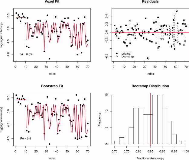
Graphical illustration of the wild bootstrap on a single voxel where b = 0 for indices 1–10 and b = 700 s/mm² for indices 11–70; (a) observations and fitted values from the diffusion tensor, (b) original and bootstrap residuals from the model fit, (c) bootstrap observations with new fitted values, and (d) bootstrap distribution of fractional anisotropy. [Color figure can be viewed in the online issue, which is available at www.interscience.wiley.com.]

MATERIALS AND METHODS

Simulation of DTI Data

Signal intensities, assumed to be taken from magnitude images, for single voxels were simulated using two sources of uncertainty. Euler angles of the principal eigenvector were drawn from a normal (Gaussian) distribution with mean µ = 45° and variance σ ² = 9°. Measurement error was drawn from the Rician distribution for each gradient direction with a signal‐to‐noise ratio of SNR ∈ {5,10,20} for the b = 0 images. Sampling from the Rician distribution is relatively straightforward, computationally, because of its relationship to the noncentral χ ² distribution with two degrees of freedom and the fact that random number generators for the noncentral χ ² distribution are widely available. Three sets of simulations were performed, one for each type of tensor: prolate (λ₁, λ₂, λ₃) = (1.5, 0.4, 0.4) μm²/ms, oblate (λ₁, λ₂, λ₃) = (0.9, 0.8, 0.6) μm²/ms, and isotropic (λ₁, λ₂, λ₃) = (0.767, 0.767, 0.767) μm²/ms. All tensor models have the same trace, Σ_i λ_i = 2.3 μm²/ms, and are based on previously reported normal values [Pierpaoli et al., 1996].

The first stage of the simulation procedure produced 1,000 Monte Carlo simulations in order to obtain sufficient “ground truth” for comparison with the proposed bootstrap techniques. A single realization from the Monte Carlo sample was drawn at random and 999 bootstrap iterations were computed based on that realization. Summary statistics, based on the eigenvalues (or functions of them) and eigenvectors, were computed for each set of MC and bootstrap realizations. This first stage was performed 250 times to provide a measure of uncertainty in the MC and bootstrap procedures. Thus, a total of 1,000 × 250 = 250,000 iterations were run and summaries of the simulation‐based results involve 250 values for each statistic of interest.

Two simulation scenarios were considered (all with b = 700 s/mm² unless otherwise specified): one with a modest number of acquisitions, 14 in total, either two b = 0 and 12 diffusion‐weighted with six gradient directions (NEX = 10) or two b = 0 and 12 diffusion‐weighted with 12 gradient directions [Jones et al., 1999b]; and one with a relatively large number of acquisitions, 70 in total, either 10 b = 0 and 60 diffusion‐weighted with six gradient directions (NEX = 10) or 10 b = 0 and 60 diffusion‐weighted with 60 gradient directions. When implementing the regular bootstrap on the 6‐direction data (NEX = 10), each regular bootstrap realization produced 70 diffusion‐weighted images (10 T2 + 60 diffusion‐weighted) drawn with replacement from the original 70 images. Similarly, when NEX = 2 each regular bootstrap realization produced 14 diffusion‐weighted images (2 T2 + 12 diffusion‐weighted) drawn with replacement from the original 14 images.

The sampling scheme proposed in this article is equivalent to the specific case of r _i = n _i, for all i, using the notation from Pajevic and Basser [2003] and corresponds exactly with the bootstrap method provided in Heim et al. [2004]. When implementing the wild bootstrap on the 60‐direction data, the two‐point distribution F ₂ was used exclusively to generate ϶; the heteroscedasticity consistent covariance matrix estimator used was where h is the diagonal element vector from the hat matrix) and u = y−X d̂ defined the residual vector.

Human MR Imaging

Data were acquired from one normal subject (28‐year‐old male Caucasian) in a Siemens Allegra 3.0 Tesla scanner using a single channel head coil. The data were collected using a protocol approved by the Massachusetts General Hospital Internal Review Board. The participant provided informed consent in writing prior to the scan session. Two sets of images were obtained: the first consisted of 10 measurements of six gradient directions (b = 700 s/mm²) and 10 T2 images (b = 0) and the second consisted of a single measurement of 60 gradient directions (b = 700 s/mm²) and 10 T2 images (b = 0). For both scans, however, the slice prescription was identical: 64 slices acquired in the AC‐PC plane, TR/TE = 7,900/83 ms, g _max = 31 mT/m, FoV = 256 × 256, base resolution = 128 × 128, 8.0 mm³ isotropic voxels. Acquisition time for each scan was 9:21. The specific choices required to implement the wild bootstrap were identical to the simulated DTI data. Note that cardiac gating was not used in the acquisition protocol.

Computational Details

To clarify notation and terminology, we use the term multiple linear regression model to denote Eq. (1). We reserve the term “multivariate” for the model below. Putting aside, for the moment, the resampling of residuals here we focus on estimating the diffusion tensor for a large number of voxels. There are clear advantages in the computational efficiency of DTI data analysis over a slice, or indeed the whole volume, when one formulates the model in Eq. (1) for all voxels as a multivariate multiple linear regression

(14)

where Y is a N × V response matrix with each column representing the log‐transformed signal intensity from a different voxel, Δ is a 7 × V matrix with each column being the diffusion tensor estimates, along with the b = 0 term. The advantage of organizing the data in this way facilitates a single application of linear algebra techniques, such as the QR or singular‐value decomposition, to estimate the diffusion tensors for all voxels simultaneously. This eliminates the need to loop over the voxels in order to perform a single multiple linear regression and produces much more efficient algorithms in common data analysis packages (such as Matlab or R) where loops, especially nested loops, are slow.

RESULTS

Simulated DTI Data

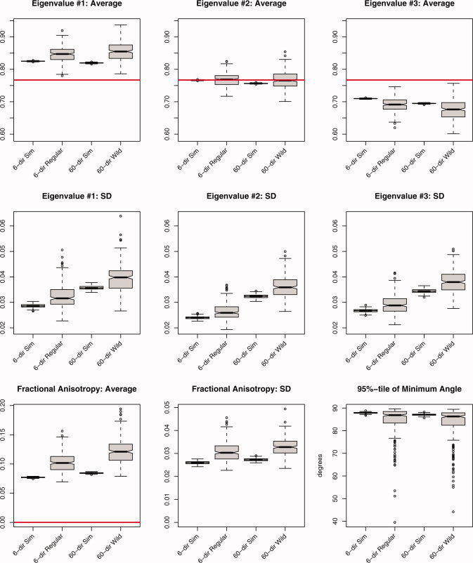
Figures 2, 3, 4 show boxplots2 of the simulation study comparing MC simulations with regular and wild bootstrap realizations for the 6‐direction data (NEX = 10) and 60‐direction data (NEX = 1) for SNR ≈ 20. Horizontal lines indicate the true value when available. The figures shown here utilize the second choice of HCCME from Eq. (8); i.e., a _i = (1–h _i)^−1/2. Simulations were performed using all three HCCMEs with no substantial difference between the characteristics of the eigenvalues or FA.

Figure 2.

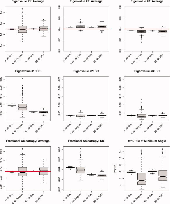
Summary statistics derived from 250 iterations of the simulation study using a prolate tensor (λ₁, λ₂, λ₃) = (1.5, 0.4, 0.4) μm²/ms, FA ≈ 0.69, SNR = 20. The average and standard deviation (SD) were computed for all three eigenvalues, fractional anisotropy, and the 95 percentile in the minimum angle subtended, under both acquisition schemes (6‐ and 60‐directions) and the three methods (Monte Carlo simulation, regular bootstrap, and wild bootstrap). The labels correspond to, from left to right, 6‐directions (NEX = 10) using MC simulation, 6‐directions (NEX = 10) using the regular bootstrap, 60‐directions using MC simulation, and 60‐directions using the wild bootstrap. [Color figure can be viewed in the online issue, which is available at www.interscience.wiley.com.]

Figure 3.

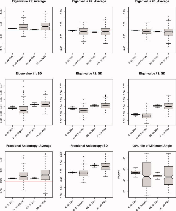
Summary statistics derived from 250 iterations of the simulation study using an oblate tensor (λ₁, λ₂, λ₃) = (0.9, 0.8, 0.6) μm²/ms, FA ≈ 0.20, SNR = 20. The average and standard deviation (SD) were computed for all three eigenvalues, fractional anisotropy, and the 95 percentile in the minimum angle subtended, under both acquisition schemes (6‐ and 60‐directions) and the three methods (Monte Carlo simulation, regular bootstrap, and wild bootstrap). The labels are identical to those in Figure 2. [Color figure can be viewed in the online issue, which is available at www.interscience.wiley.com.]

Figure 4.

Summary statistics derived from 250 iterations of the simulation study using an isotropic tensor (λ₁, λ₂, λ₃) = (0.767, 0.767, 0.767) μm²/ms, SNR = 20. The average and standard deviation (SD) were computed for all three eigenvalues, fractional anisotropy, and the 95 percentile in the minimum angle subtended, under both acquisition schemes (6‐ and 60‐directions) and the three methods (Monte Carlo simulation, regular bootstrap, and wild bootstrap). The labels are identical to those in Figure 2. [Color figure can be viewed in the online issue, which is available at www.interscience.wiley.com.]

For the prolate tensor, averages for λ₂ and λ₃ exhibit a small amount of bias due to sorting while λ₁ is much less affected [Pierpaoli and Basser, 1996]. Both regular and wild bootstrap estimates of the average show much more variability, but this is to be expected since they are based on a single observation, whereas the MC averages have 1,000 observations. Standard deviations of the eigenvalues indicate a difference in sampling schemes, although not enough to be clinically meaningful. The regular bootstrap estimates of the eigenvalue SD are negatively biased for the 6‐direction scheme and are much more variable than the wild bootstrap results for the 60‐direction scheme, even though the former has 10 measurements per gradient direction. This may be due purely to the number of directions sampled, not the bootstrap methodology, with the 60‐direction scheme producing more stable estimates of the diffusion tensor elements from which these eigenvalues are based; as noted previously by Jones [2004].

One potential source of variability comes from the fact that the regular and wild bootstrap procedures were applied to separate data sets. An additional step was included where the wild bootstrap was applied to the data from the 6‐direction scheme without altering the algorithm. No difference in performance, as measured by estimates of the average and SD of the eigenvalues, was detected when the wild bootstrap was applied to the data from the 6‐direction scheme compared to the regular bootstrap procedure.

Average fractional anisotropy (FA) is accurately estimated by the wild bootstrap for 60‐direction data with increased precision when compared with the regular bootstrap for the 6‐direction data (the true value of FA is ∼0.69). The SD of estimated FA values is less for the 60‐direction scheme and its bootstrap estimate of SD appears to be much less biased than the results from the regular bootstrap on the 6‐direction scheme. When looking at the so‐called cone of uncertainty [Jones, 2003], neither bootstrap technique adequately estimates the 95 percentile from the MC simulations. Instead, both techniques are at least 2° less (20%) when comparing median values (solid bar in the boxplot) with the MC simulation results. Such discrepancies, between the MC simulations and bootstrap samples, are not apparent in the other univariate summaries of the diffusion tensor model displayed but those quantities are inherently more stable; e.g., the mean and standard deviation. Given that the bootstrap estimates of the 95 percentile are based on a single realization of the prolate tensor model, instead of 1,000 realizations, there is not enough information to accurately reproduce more difficult quantities such as extreme values.

The oblate tensor in Figure 3 shows the usual sorting bias in the average for all three eigenvectors by both bootstrap methods, with similar precision but slightly more bias in λ₁ and λ₃ for the wild bootstrap. The regular bootstrap for the 6‐direction data and the wild bootstrap for the 60‐direction data produced similar quality estimates of eigenvalue SD for all three eigenvalues, with a slight negative bias in the regular bootstrap. This is likely due to the number directions in the encoding scheme and not specifically attributable to the bootstrap methodology. Average FA shows a slight positive bias for both sampling schemes, with the wild bootstrap on the 60‐direction data being less precise when compared with the regular bootstrap applied to the 6‐direction data. The SD of estimated FA shows only minor differences between the two bootstrap procedures, with a slight negative bias for the wild bootstrap. Estimates of angular difference for the cone of uncertainty are much improved versus the prolate tensor. Both bootstrap methods demonstrate a negative bias when estimating the 95 percentile of the minimum angle subtended; this is similar to the case of the prolate tensor and is most likely due to the difficulties in estimating extremes from the bootstrap applied to a single realization.

The isotropic tensor in Figure 4 exhibits pronounced effects from sorting bias in the eigenvalues. Both bootstrap techniques suffer from increased bias, positive for λ₁ and negative for λ₃, when compared with the MC simulations. When comparing estimates of the SD for each eigenvalue, the 60‐direction scheme exhibits a larger SD, both in simulation and through the wild bootstrap, but the positive bias from the wild bootstrap does not appear to be much larger than the positive bias present in the regular bootstrap for the 6‐direction data. The true FA for all simulations is zero, but with the inclusion of Rician noise this is not possible to attain and thus positive bias in estimates of FA (whether from MC or bootstrap realizations) is to be expected. Bias from the true value of zero is around 0.08 for the MC simulations, a little less for the 6‐direction scheme, and the bootstrap realizations exhibit positive bias above and beyond that to be expected from the MC results (on the order of 0.02–0.04 units FA). The estimated SD of FA was very similar for the two sampling schemes for the MC simulations, with a slight positive bias when applying the bootstrap techniques. The wild bootstrap does exhibit increased bias when compared with the regular bootstrap. This is most likely due to the encoding scheme and not the bootstrap methodology. With 10 acquisitions under the six‐direction scheme, there is more information about the variability of the data instead of a single acquisition with 60 directions. Thus, the wild bootstrap, based on the 60‐direction data, is exhibiting increased variability when estimating FA. The 95 percentile of the angular difference is very close to 90 degrees, with a small negative bias for the bootstrap techniques and a large left‐hand tail in the observed distribution of angles.

When the SNR was reduced to 5 or 10, the performances of the regular and wild bootstrap methods, relative to their MC simulations, follow the patterns observed in Figures 2, 3, 4 with a few notable differences (not shown). For the prolate tensor, decreased SNR induces substantial negative bias in the estimated major eigenvalue when using only six directions, and thus, negative bias in FA. This is not observed in estimates obtained from the 60‐direction data. The ability of either bootstrap method to accurately reproduce the uncertainty in the angular difference is much better; a negligible bias is observed when compared with high SNR. Patterns in the performance of either bootstrap method did not appear to be differentially affected by decreasing SNR for the oblate and isotropic tensors.

Human DTI Data

Statistical summaries of fractional anisotropy (FA) color map and bootstrap standard error (SE), in grayscale, for axial slices through the centrum semiovale (Fig. 5, panels a–e, a‘–e’; k–o, k‘–o’) and through the caudal midbrain/rostral pons (Fig. 5, panels f–j, f‘–j’; p–t, p‘–t’) are displayed for both the 6‐ and 60‐direction data. Minor differences between the two sampling schemes for the estimated FA, colored by the direction of the principal eigenvector [Pajevic and Pierpaoli, 1999], are apparent.

Figure 5.

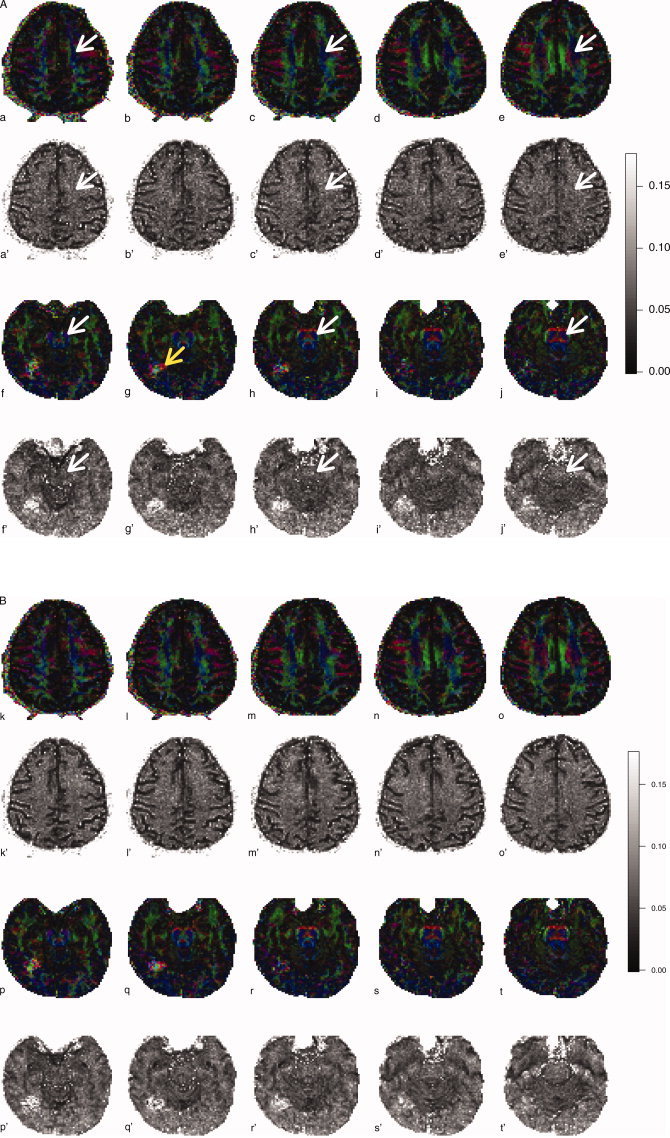
Fractional anisotropy, colored by principal eigenvector, for a single subject scanned using both 6‐direction and 60‐direction sequences. Standard errors from the regular bootstrap are provided for the 6‐direction sequence and from the wild bootstrap for the 60‐direction sequence. Both sets of bootstrap SEs are displayed in FA units (ranging from 0 to 0.175). Centrum semiovale (top rows) and caudal midbrain/rostral pons (bottom rows) are demarcated on alternating slices of the 6‐direction sequence only (white arrows). A region of FA disruption can be seen in the inferior temporal lobe near the fusiform gyrus (yellow arrow).

From motor cortex, the corticospinal tracts travel inferiorly through

• 1centrum semiovale in the cerebral hemispheres,
• 2posterior limb of the internal capsule,
• 3cerebral peduncles of the midbrain, and
• 4pons before reaching the medulla to form the pyramids.

The axial views in Figure 5 demonstrate the corticospinal tracts in the cerebral hemispheres and brainstem. Although the corticospinal tracts are well defined in the cerebral peduncles, they are not as well defined in the areas of the centrum semiovale and pons where other white matter tracts intersect. To illustrate, the FA color map shows the centrum semiovale as a mostly “blue” structure (oriented in the superior‐inferior direction) in superior slices, but intersecting “red” fibers (oriented left‐right) can be seen in inferior slices (Fig. 5, panels a–e, white arrows). Arrows are only shown on every other slice and in the six‐direction data only for simplicity. A similar trend is shown in the transition from the caudal midbrain to the rostral pons (Fig. 5, panels f–j). Thus, we expected that lower bootstrap SE would be found in voxels corresponding to the corticospinal tracts of the cerebral peduncles as compared to either the centrum semiovale or rostral pons in both the 6‐ and 60‐direction data. Figure 5, panels a‘−e’ and f‘−g’ show that this is indeed the case, although the results are more apparent in the brainstem. Figure 6, a map of the bootstrap SE for the principal eigenvector Euler angle, accentuates the results from SE maps in Figure 5 and emphasizes the results that angular uncertainty is low in regions where the white matter bundles are uniform in direction and high in regions where white matter bundles intersect (red arrows shown on every other slice and in the six‐direction data only for simplicity). This agrees with previous results when using the regular bootstrap [Jones, 2003].

Figure 6.

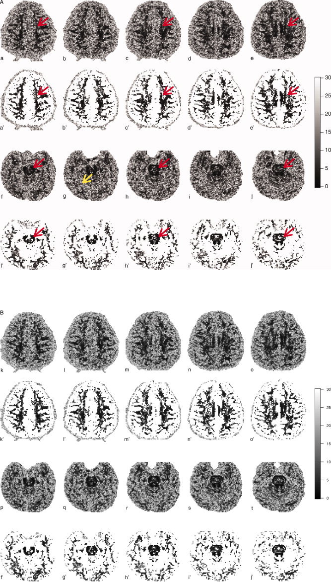
Bootstrap estimates of the standard error (SE) for the principal eigenvector Euler angle, obtained from the regular bootstrap for the 6‐direction acquisition and from the wild bootstrap for the 60‐direction acquisition. The first and third rows show all values from 0° ≤ SE ≤ 30° and the second and fourth rows only displays voxels with an FA > 0.4. Centrum semiovale (top rows) and caudal midbrain/rostral pons (bottom rows) are demarcated on alternating slices of the 6‐direction sequence only (red arrows). The region of FA disruption in the inferior temporal lobe near the fusiform gyrus that was seen in the FA color map is delineated by the yellow arrow.

Although these data were obtained from a healthy control subject, we found a single, unexpected hypointensity in the region of the inferior temporal lobe near the fusiform gyrus in the b = 0 scan (data not shown; the lesion was reported to the subject, who was encouraged to obtain a follow‐up with his physician). Follow‐up T2 and FLAIR scans failed to show any edema or white matter hyperintensity, respectively, in the vicinity of the lesion. Interestingly, the color maps show an apparent disruption in the FA surrounding the lesion (Fig. 5g, yellow arrow), and the bootstrap maps, both regular and wild, indicate an increase in the SE. However, the Euler angle map (Fig. 6g) fails to show any remarkable difference in the SE of this region.

It should be noted that cardiac gating was not used in the acquisition of these data. Hence, quantification and visualization of effects attributable to cardiac pulsation is not possible. The fact that the wild bootstrap operates on a single set of measurements means that implementing cardiac gating will not necessarily improve its performance. The regular bootstrap, by definition, requires several measurements and is therefore able to take advantage of such DTI acquisition schemes. One procedure is not necessarily optimal for all situations and caution should be exercised when deciding on the specific DTI acquisition scheme, not only for data quality implications but also its impact on data modeling and analysis.

DISCUSSION AND CONCLUSIONS

A collection of resampling techniques has been proposed, which provides estimates of uncertainty in univariate summaries of the estimated diffusion tensor, regardless of the specific DTI acquisition method assuming that more than six gradient directions have been acquired or a six‐direction gradient encoding scheme has been acquired more than once. The performance of model‐based resampling schemes show no loss of precision or accuracy when compared with the well‐established regular bootstrap procedure in both simulations and human DTI data. It should be noted that a negative bias (on the order of 20%) was found in the cone of uncertainty for simulated prolate tensors when a large number (e.g., 60) of diffusion‐weighted images are acquired, but not found in oblate or isotropic tensor models, regardless of the bootstrap method used. The reason for this is not clear at the moment, but it should be noted that this disappeared with reduced SNR in simulations. For prolate tensors, any bootstrap method based on six‐direction data produced highly variable estimates of FA when compared to the 60‐direction data. This result reiterates the advantages of using a larger number of gradient directions, even if only one measurement is taken per direction.

Given the fact that errors in the linear regression model of log‐transformed signal intensity are not Gaussian, nor symmetric, the choice of resampling distribution (F ₁ or F ₂) may have an impact on the wild bootstrap. Bose and Chatterjee [2002] compared variance estimates of regression parameters under several skewed error distributions. The wild bootstrap was found to be inferior when compared to alternative methods. However, in simulation studies with highly skewed errors (from a noncentral χ${}_{\text{2}}^{\text{2}}$ distribution) the wild bootstrap using F ₂ performed similarly to F ₁, and never worse when comparing errors in rejection probabilities [Davidson and Flachaire, 2001]. Both resampling distributions were applied in simulation studies with no visible difference between the estimated diffusion tensor models or in univariate summaries of the diffusion tensor. In most, if not all, of the simulations performed for DTI data analysis here the wild bootstrap for single‐average acquisitions performed as well as the regular bootstrap for multiple acquisitions. Additional simulation studies were also conducted in which the heteroscedasticity consistent covariance matrix estimator (HCCME) was varied between three choices in the literature. No substantial differences in the performance of the wild bootstrap were observed when duplicating the simulation studies on prolate, oblate, and spherical tensor models using the three HCCME's proposed in the section on Model‐Based Resampling: Homoscedastic Errors.

Simulations were also performed to investigate the resampling‐within‐gradient‐directions (RWGD) and wild bootstrap applied to the six‐direction sampling scheme with SNR ≈ 20 (not shown here). For all three tensor models (prolate, oblate, and isotropic) the RWGD and wild bootstrap techniques exhibited minor differences in bias for statistical summaries of the eigenvalues, and thus, fractional anisotropy when compared with the regular bootstrap. However, these differences were not great nor did they follow an obvious pattern. The bootstrap techniques (regular, model‐based, and wild) produced essentially identical results when applied to the six‐direction clinical data. A slight reduction in bias for the 95 percentile of the angular difference was observed for the RWGD and wild bootstrap, most notable in the oblate tensor model, but these were in the order of 5–10% compared with the simulated angular difference. These results provide an empirical validation of both model‐based bootstrap techniques compared to the established regular bootstrap for a variety of clinically relevant tensors.

Not all DTI acquisition protocols can accommodate 60 diffusion‐weighted images per scan, whether or not those images come from a low number of gradient directions with a large NEX or a high number of gradient directions with a low NEX. Figure 7 summarizes a simulation study where the performance of the regular and wild bootstraps for the six‐direction data (NEX = 2) and 12‐direction data (NEX = 1) were compared with MC simulations for SNR ≈ 20. Individual eigenvalue results have been omitted and only FA and the 95 percentile of the minimum angle subtended are shown. Results on estimating the average FA value follow the same trends established with looking at six‐direction data with NEX = 10. That is, the prolate tensor is well estimated and the oblate and isotropic tensors exhibit substantial positive bias. The bias is even more pronounced since only a fraction of the data (20%) are available for both the MC simulations and bootstrap procedures compared to the MC simulations using a total of 70 acquisitions per scan. The wild bootstrap performed better, in general, in estimating the SD of FA in all three tensor models when compared with the regular bootstrap on the six‐direction data and also performed well with the 12‐direction data. This may be because the wild bootstrap adds variability by flipping the residuals, thus causing more variability than simply resampling such a low number (two) of acquisitions per gradient direction. For the minimum angle subtended, the wild bootstrap performs well for both the 6‐ and 12‐direction data and the regular bootstrap consistently underestimates the 95 percentile.

Figure 7.

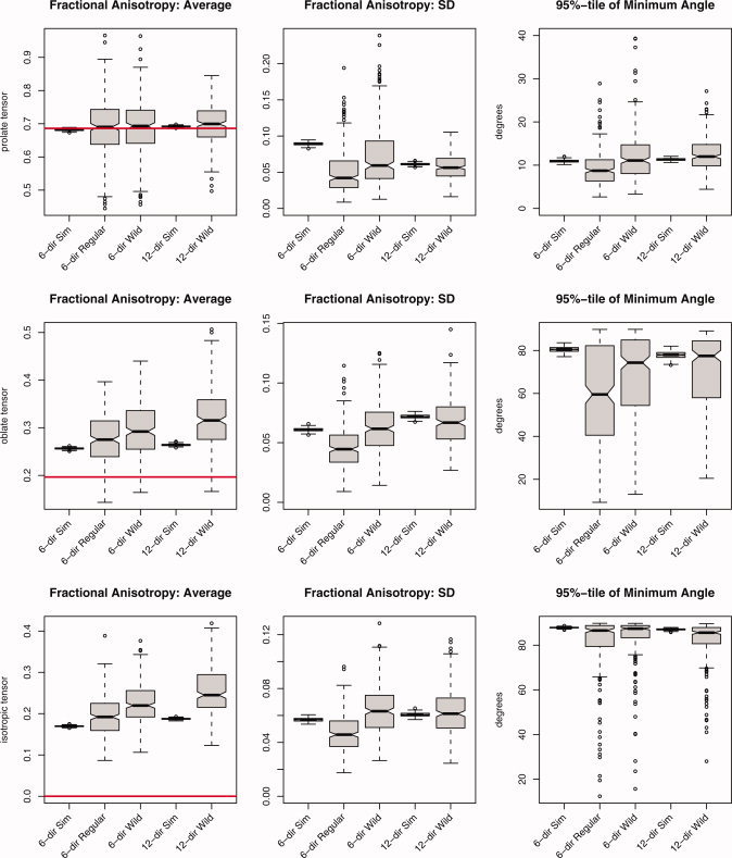
Summary statistics for fractional anisotropy and the 95 percentile in the minimum angle subtended derived from 250 iterations of the simulation study using all three diffusion tensor models (prolate, oblate, and isotropic), SNR = 20. The labels correspond to, from left to right, 6‐directions (NEX = 2) using MC simulation, 6‐directions (NEX = 2) using the regular bootstrap, 6‐directions (NEX = 2) using the wild bootstrap, 12‐directions using MC simulation, and 12‐directions using the wild bootstrap. [Color figure can be viewed in the online issue, which is available at www.interscience.wiley.com.]

The linear model identified in Eq. (1) is used to estimate the diffusion tensor elements, and thus, infer the white matter integrity at a voxel level. The true relationship between signal intensity and the parameters of the diffusion tensor model is a nonlinear one, the log transform is one way to place the estimation problem onto the solid foundation of a linear model, at the cost of transforming the noise distribution [Salvador et al., 2005]. Given the ever‐increasing capabilities of computing resources, it is fair to ask why parameter estimation does not take place directly on the nonlinear model. Arguments in favor of the linear model are that linear models have a direct solution via the theory of least squares, computation is efficient and may be parallelized so that the diffusion tensor elements for all are estimated simultaneously (see the Computational Details section), and optimization algorithms involve user‐defined starting values and may not converge. We have offered model‐based resampling in the linear regression model as a straightforward statistical technique that offers researchers the ability to generate empirical errors on quantities of interest in the familiar framework of the diffusion tensor model. We acknowledge that the linear regression model is suboptimal as the signal‐to‐noise ratio goes down, especially since finer spatial resolution is sought after, and are currently investigating estimation techniques that respect the physical model and distribution of the noise.

Although we have focused on a small set of scalar summaries of the diffusion tensor there are two areas of application in DTI that may benefit from the proposed methodology. Firstly, more complicated models based on the Gaussian model of diffusion are amenable to the bootstrap but additional work is required to incorporate heteroscedasticity [Basford et al., 1997; Tuch et al., 2002]. Semiparametric or nonparametric models of diffusion at the voxel level, such as q‐ball imaging [Tuch, 2004], will require careful application of bootstrap methodology. The q‐ball reconstruction may also be interpreted in a linear regression framework. The challenge will be to describe the angular and anisotropy variability when there are multiple peaks. Also, since the orientation distribution function (ODF) is treated as a probability density, one would need a framework to describe the fact that the probability density is due to both the physical model and the bootstrap variability. Secondly, the regular bootstrap has already been applied to the area of fiber tractography [Jones and Pierpaoli, 2005; Jones et al., 2005; Lazar and Alexander, 2005]. Application of the wild bootstrap, instead of the regular bootstrap, is possible when the diffusion tensor is estimated from the DTI data using the model of Basser et al. [1994] with preliminary results already presented [Jones, 2006].

By applying the bootstrap to the errors from the linear regression model relating observed signal intensity to the diffusion tensor, we have provided an alternative to the most common method to estimate a diffusion tensor in MRI. When applied to clinical data with several measurements per gradient direction, the regular bootstrap and model‐based bootstrap perform equally well, thus giving the researcher a choice in implementation without sacrificing the accuracy nor the precision for estimates of uncertainty. Even when only a single measurement is available for each gradient direction, the wild bootstrap may be applied to obtain estimates of uncertainty assuming that more than six gradient directions have been acquired or a six‐direction gradient encoding scheme has been acquired more than once.

REFERENCES

- Anderson AW( 2001): Theoretical analysis of the effects of noise on diffusion tensor imaging. Magn Reson Med 46: 1174–1188. [DOI] [PubMed] [Google Scholar]
- Basford KE, Greenway DR, McLachlan GJ, Peel D( 1997): Standard errors of fitted means under normal mixture models. Comput Stat 12: 1–17. [Google Scholar]
- Basser PJ, Mattiello J, LeBihan D( 1994): Estimation of the effective self‐diffusion tensor from the NMR spin echo. J Magn Reson 103: 247–254. [DOI] [PubMed] [Google Scholar]
- Batchelor PG, Atkinson D, Hill DLG, Calamante F, Connelly A( 2003): Anisotropic noise propagation in diffusion tensor MRI sampling schemes. Magn Reson Med 49: 1143–1151. [DOI] [PubMed] [Google Scholar]
- Behrens TEJ, Woolrich MW, Jenkinson M, Johansen‐Berg H, Nunes RG, Clare S, Matthews PM, Brady JM, Smith SM( 2003): Characterization and propogation of uncertainty in diffusion‐weighted MR imaging. Magn Reson Med 50: 1077–1088. [DOI] [PubMed] [Google Scholar]
- Bose A, Chatterjee S ( 2002): Comparison of bootstrap and jackknife variance estimators in linear regression: Second order results. Stat Sin 12: 575–598. [Google Scholar]
- Davidson R, Flachaire E( 2001): The wild bootstrap, tamed at last. Working Paper IER#1000, Queen's University.
- Davison AC, Hinkley DV( 1997): Bootstrap Methods and their Application. Cambridge, UK: Cambridge University Press. [Google Scholar]
- Efron B( 1981): Nonparametric estimates of standard error: The jackknife, the bootstrap and other methods. Biometrika 68: 589–599. [Google Scholar]
- Efron B, Tibshirani R( 1993): An Introduction to the Bootstrap. New York: Chapman & Hall. [Google Scholar]
- Flachaire E( 2005): Bootstrapping heteroskedastic regression models: wild bootstrap vs. pairs bootstrap. Comput Stat Data Anal 49: 361–376. [Google Scholar]
- Hasan KM, Narayana PA( 2003): Computation of the fractional anistropy and mean diffusivity maps without tensor decoding and diagonalization: Theoretical analysis and validation. Magn Reson Med 50: 589–598. [DOI] [PubMed] [Google Scholar]
- Heim S, Hahn K, Sämann PG, Fahrmeir L, Auer DP( 2004): Assessing DTI data quality using bootstrap analysis. Magn Reson Med 52: 582–589. [DOI] [PubMed] [Google Scholar]
- Jones DK( 2003): Determining and visualizing uncertainty in estimates of fiber orientation from diffusion tensor MRI. Magn Reson Med 49: 7–12. [DOI] [PubMed] [Google Scholar]
- Jones DK( 2004): The effect of gradient sampling schemes on measures derived from diffusion tensor MRI: A Monte Carlo study. Magn Reson Med 51: 807–815. [DOI] [PubMed] [Google Scholar]
- Jones DK( 2006): Tractography gone wild: Probabilistic tracking using the wild bootstrap. In Proceedings of the 14th Annual Meeting of ISMRM, Seattle, pp 435.
- Jones DK, Basser PJ( 2004): “Squashing peanuts and smashing pumpkins”: How noise distorts diffusion‐weighted MR data. Magn Reson Med 52: 979–993. [DOI] [PubMed] [Google Scholar]
- Jones DK, Pierpaoli C( 2005): Confidence mapping in diffusion tensor magnetic resonance imaging tractography using a bootstrap approach. Magn Reson Med 53: 1143–1149. [DOI] [PubMed] [Google Scholar]
- Jones DK, Horsfield MA, Simmons A( 1999a): Optimal strategies for measuring diffusion in anisotropic systems by magnetic resonance imaging. Magn Reson Med 42: 515–525. [PubMed] [Google Scholar]
- Jones DK, Simmons A, Williams SC, Horsfield MA( 1999b): Non‐invasive assessment of axonal fiber connectivity in the human brain via diffusion tensor MRI. Magn Reson Med 42: 37– 41. [DOI] [PubMed] [Google Scholar]
- Jones DK, Travis AR, Eden G, Pierpaoli C, Basser P( 2005): PASTA: Pointwise assessment of streamline tractography attributes. Magn Reson Med 53: 1462–1467. [DOI] [PubMed] [Google Scholar]
- Lazar M, Alexander AL( 2005): Bootstrap white matter tractography (BOOT‐TRAC). Neuroimage 24: 524–532. [DOI] [PubMed] [Google Scholar]
- Liu RY( 1988): Bootstrap procedure under some non‐i.i.d. models. Ann Stat 16: 1696–1708. [Google Scholar]
- MacKinnon JG, White HL( 1985): Some heteroskedasticity consistent covariance matrix estimators with improved finite sample properties. J Econometrics 21: 53–70. [Google Scholar]
- Mammen E( 1993): Bootstrap and wild bootstrap for high dimensional linear models. Ann Stat 21: 255–285. [Google Scholar]
- O'Gorman RL, Jones DK( 2005). How many bootstraps make a buckle?In Proceedings of the 13th Annual Meeting of ISMRM, Miami Beach, pp 225.
- Pajevic S, Basser PJ( 2003): Parametric and non‐parametric statistical approaches in diffusion tensor magnetic resonance imaging. J Magn Reson 161: 1–14. [DOI] [PubMed] [Google Scholar]
- Pajevic S, Pierpaoli C( 1999): Color schemes to represent fiber orientation of anisotropic tissues from diffusion tensor data: Application to white matter fiber tract mapping in the human brain. Magn Reson Med 42: 526–540. [PubMed] [Google Scholar]
- Pierpaoli C, Basser P( 1996): Toward a quantitative assessment of diffusion anisotropy. Magn Reson Med 36: 893–906. [DOI] [PubMed] [Google Scholar]
- Pierpaoli C, Jezzard P, Basser PJ, Barnett A, Di Chiro G( 1996): Diffusion tensor MR imaging of the human brain. Radiology 201: 637–648. [DOI] [PubMed] [Google Scholar]
- Poonawalla AH, Zhou XJ( 2004): Analytical error propogation in diffusion anisotropy calculations. J Magn Reson Imaging 19: 489–498. [DOI] [PubMed] [Google Scholar]
- Salvador R, Peña A, Menon DK, Carpenter TA, Pickard JD, Bullmore ET( 2005): Formal characterization and extension of the linearized diffusion tensor model. Hum Brain Mapp 24: 144–155. [DOI] [PMC free article] [PubMed] [Google Scholar]
- Skare S, Li T‐Q, Nordell B, Ingvar M( 2000): Noise considerations in the determination of diffusion tensor anisotropy. Magn Reson Imaging 18: 659–669. [DOI] [PubMed] [Google Scholar]
- Tuch DS( 2004): Q‐ball imaging. Magn Reson Med 52: 1358–1372. [DOI] [PubMed] [Google Scholar]
- Tuch DS, Reese TG, Wiegell MR, Makris N, Belliveau JW, Wedeen VJ( 2002): High angular resolution diffusion imaging reveals intravoxel white matter fiber heterogeneity. Magn Reson Med 48: 577–582. [DOI] [PubMed] [Google Scholar]
- Whitcher B, Tuch DS, Wang L( 2005). The wild bootstrap to quantify variability in diffusion tensor MRI. In Proceedings of the 13th Annual Meeting of ISMRM, Miami Beach, pp 1333.