Random fields—Union intersection tests for detecting functional connectivity in EEG/MEG imaging

Abstract

Electrophysiological (EEG/MEG) imaging challenges statistics by providing two views of the same underlying spatio‐temporal brain activity: a topographic view (EEG/MEG) and tomographic view (EEG/MEG source reconstructions). It is a common practice that statistical parametric mapping (SPM) for these two situations is developed separately. In particular, assessing statistical significance of functional connectivity is a major challenge in these types of studies. This work introduces statistical tests for assessing simultaneously the significance of spatio‐temporal correlation structure between ERP/ERF components as well as that of their generating sources. We introduce a greatest root statistic as the multivariate test statistic for detecting functional connectivity between two sets of EEG/MEG measurements at a given time instant. We use some new results in random field theory to solve the multiple comparisons problem resulting from the correlated test statistics at each time instant. In general, our approach using the union‐intersection (UI) principle provides a framework for hypothesis testing about any linear combination of sensor data, which allows the analysis of the correlation structure of both topographic and tomographic views. The performance of the proposed method is illustrated with real ERP data obtained from a face recognition experiment. Hum Brain Mapp 2009. © 2009 Wiley‐Liss, Inc.

INTRODUCTION

Functional connectivity in hemodynamic and electromagnetic data is usually interpreted as the temporal correlation between spatially remote neurophysiological events [Friston et al., 1993; Friston, 1996]. This concept can be extended to any other image measurements by saying, for instance, that two different regions of the brain are “functionally” connected if they show similar anatomical features over subjects [Worsley et al., 2005]. Several approaches have been proposed for assessing functional connectivity in images based on hemodynamic measurements [Baumgartner et al., 2000; Cao and Worsley, 1999; Koch et al., 2002; Van de ven et al., 2004; Worsley et al., 2005], electrophysiological (EEG/MEG) recordings [Gevins, 1989; Urbano et al., 1998], as well as multimodal integration data [Babiloni et al., 2005]. Typically, such approaches are based on the estimation of the covariance (or correlation) structure between time series measured at different spatial locations. However, most of them are constrained by the obvious limitations of the spatial and temporal resolutions of the corresponding measurements. As a consequence, those recording modalities producing high spatio‐temporal resolution images would be suitable candidates for an effective dynamic (time‐varying) functional connectivity analysis.

Recent years have witnessed the emergence of a number of methods for the analysis of high resolution EEG/MEG data characterized by the use of a high number of scalp electrodes/coils located on/over the scalp. The high temporal resolution of these types of electromagnetic measurements offers invaluable information about the neuronal activation dynamics, which complements the detailed spatial information provided by other imaging modalities, such as PET or fMRI. These techniques, however, pose new challenges to the statistics of functional connectivity in the spaces of both the sensors and underlying sources. In the first case, one is interested in detecting significant correlations between the components of the event related potential/event related field (ERP/ERF) and their topographic distribution, that is, the spatio‐temporal correlation structure of the ERP/ERF components in high dimensional EEG/MEG data. In the second case, however, one focuses on explaining the underlying ERP/ERF correlation structure in terms of the current sources generating the corresponding components. These current sources can be estimated by solving the inverse problem of the EEG/MEG [Pascual‐Marqui et al., 2002; Trujillo‐Barreto et al., 2004].

Different approaches have been followed for the analysis of connectivity in both the topographic (“sensors/coils” space) and the tomographic (“sources” space) views of EEG/MEG data. On the one hand, a number of linear and nonlinear connectivity measures have been proposed for analyzing the spatio‐temporal topographic correlation structure of ERP/ERF components [see e.g. David et al., 2004; Koenig et al., 2005]. Examples are: multi‐channel EEG/MEG cross‐correlation coefficients (or coherence in the frequency domain) [Gevins and Remond, 1987; Schindler et al., 2007], directed transfer function (DTF) [Kaminski et al., 2001], mutual information, and nonlinear correlation. On the other hand, some of these measures have been adapted for analyzing connectivity in the current density sources domain [Astolfi et al., 2007; Thatcher et al., 2007]. But one could also, in principle, use any of the methods available for PET, MRI, and fMRI images.

Nevertheless, a common feature of all these approaches is that they use different criteria for assessing the statistical significance of functional connectivity in topographic as opposed to tomographic data. In fact, they employ statistical tests derived from different principles in each case, and almost none of them provide a decision threshold for statistical significance in a classical hypothesis testing framework. In this work, this issue is addressed by presenting a blend of techniques that provides a global decision threshold for detecting changes in the time‐varying correlation structure between ERP/ERF components recorded on two different scalp regions. Then, it is shown that the same threshold can be used for assessing the statistical significance of hypotheses in both the topographic and tomographic correlation structure of such components. This is done by applying the classical statistical parametric mapping (SPM) approach based on random field theory (RFT).

Additionally, as pointed out by [Kiebel and Friston, 2004], there is a severe limitation when using space‐time SPM for ERP/ERF studies. In fact, it is very difficult to make inferences about the temporal extent of the evoked responses within the spatiotemporal SPM framework. Thus, in most of the cases, it is necessary to make inferences over time explicitly. In this article, we model our spatio‐temporal ERP/ERF data as a multivariate response at each time instant and make inferences in the context of “temporal” SPM. In particular, we follow the same approach used in [Carbonell et al., 2004]. That is, RFT is used for solving the multiple comparison problems resulting from testing global time‐varying correlations on the sensor data. The union‐intersection (UI) principle is then applied to testing hypotheses on the tomographic and topographic views. Although they look very similar, there is a key difference between this work and the results of [Carbonell et al., 2004]. That is, the method described in [Carbonell et al., 2004] is restricted to the detection of ERP/ERF components and their corresponding current generating sources. In contrast, the approach proposed here focuses on characterizing the time‐varying correlation structure underlying such components and its explanation by the corresponding source activity.

The statistical procedure proposed in this article can be summarized as follows:

• 1Definition of the global null hypothesis of “no functional connectivity” between the ERP/ERF components generated at two spatially remote brain regions.
• 2Testing this null hypothesis by computing the multivariate greatest root statistic θ_t at each time instant t in the time window of analysis.
• 3Calculation of a global decision threshold G _α by using RFT under the assumption that the statistics of Step 2 are realizations of a 1‐dimensional random field. This threshold can then be used for detecting “connectivity” between ERP/ERF components at the time instants where θ_t exceeds G _α.
• 4Application of UI tests for examining hypotheses about the topographic and tomographic correlation structure of the ERP/ERF components, at the significant time instants detected by Step 3.

Notice that Step 4 exploits the fact that EEG/MEG data is usually represented by vectors of voltage/field values recorded from a set of sensors, and many topographic and tomographic views are obtained by linear combinations of these vectors. This allows us to use the UI principle to test hypothesis about the time‐varying correlation structure in both the topographic and the tomographic views.

SUBJECTS AND METHODS

EEG data was acquired on a 128‐channel Biosemi ActiveTwo system, sampled at 2,048 Hz, with electrodes on the left earlobe, right earlobe, and two electrodes to measure HEOG and VEOG. The data were referenced to the average of left and right earlobe electrodes and epoched from −200 ms to +600 ms. These epochs were then detrended and examined for artifacts, defined as time points that exceeded an absolute threshold of 120 microvolt (mainly in the VEOG). The ERP data set is the same one used in [Henson et al., 2003]. The basic paradigm consists on presentation of 86 faces (43 famous and 43 novel) and 86 scrambled faces, which gives three event‐types: unfamiliar faces (U), familiar faces (F), and scrambled faces (S). The scrambled faces were created by 2D Fourier transformation, random phase permutation, inverse transformation, and outline‐masking of each face. Thus, faces and scrambled faces are closely matched for low‐level visual properties such as spatial frequency power density. Faces were presented for 600 ms, every 3,600 ms. More details about the experimental paradigm can be found at http://www.fil.ion.ucl.ac.uk/spm/data/mmfaces.html. After artifact rejection, our primary data set on conditions F, U, and S consisted of 38, 38, and 76 trials of 128 channels on each trial.

Our source space consists of a 3D grid of points that represent the putative generators of the EEG/MEG inside the brain. In turn, the measurement space is defined by the array of sensors where the EEG/MEG is recorded. In this work, 3,244 grid points (7 mm grid spacing) and the 128 EEG electrodes of the Biosemi ActiveTwo system were placed in registration with the average probabilistic MRI atlas (“average brain”) produced by the Montreal Neurological Institute [Collins et al., 1994; Evans et al., 1993; Mazziotta et al., 1995]. The 3D grid was constrained to those brain areas where the probability of grey matter was significantly greater than the probability of any other tissue type.

Data Model

Let [X]_sct be a three‐dimensional array that represents the recorded voltages corresponding to trial s, s = 1,…, S, channel c, c = 1,…, C and time instant t, t = 1,…, T. Here, S, C, and T denote the number of trials, channels, and time instants, respectively. A common model for such ERP data [Aunon et al., 1981] assumes that the recorded voltage values [X]_sct are the superposition of the ERP (signal μ_ct) and a background brain activity or noise (e _sct) noncontingent to the stimuli, that is,

where the vectors e _st = (e_s1t,…,e_sCt) are assumed to be statistically independent across trials and normally distributed with zero mean and (typically unknown) covariance matrix Σ_t.

Notice that in typical functional connectivity studies, independent observations come from residual data images at different time points, which results from fitting a linear model for removing nuisance effects (drift, constant terms) and temporal correlations (usually referred to as whitening). In contrast, the previous model takes into account temporal correlations by making explicit the time dependence of the parameters Σ_t and μ_ct. Independent observations come from the independent trials (repetitions) obtained in a typical ERP/ERF experiment. Hence, in what follows, we are going to use the term “time‐varying” to emphasize the temporal dependence of the model parameters as well as of their corresponding statistical tests. In fact, the aim of this article is to characterize (by statistical hypothesis testing) the time‐varying structure of the covariance matrix Σ_t by means of statistical hypothesis testing.

Note that the temporal dependence of the model parameters will only be used to correct the inference, and it will not be used for parameter estimation. This is actually the procedure used in mass univariate SPM approaches [Kiebel and Friston, 2004]. Under this assumption, the maximum likelihood estimators of the mean μ_t = (μ_1t,…, μ_Ct) and the covariance matrix Σ_t are given by

and

where x _st = (X _s1t,…, X _sCt)′, respectively.

Statistics for Functional Connectivity

As in the classical problem of detecting ERP/ERF components, it would be desirable to obtain an analogous solution for the problem of detecting functional connectivity between these components. This entails detecting changes in the time‐dependent spatial correlation structure of ERP/ERF components.

To solve this problem, one would like to test, in principle, the null hypothesis that Σ_t is a diagonal matrix at all time instants t. However, it is well‐known that the relationship between current density sources inside the brain and the EEG/MEG measurements outside the head is determined by volume conduction properties and the geometry of the different tissue types inside the head. Indeed, even the simple case of a single dipolar source would produce a widely dispersed voltage distribution over a large region on the scalp surface. This produces high correlation values between spatially close scalp measurements. Hence, the type of null hypothesis described above would be rejected in most of the cases, in particular in those with high density multi‐channel recordings.

A more realistic hypothesis testing would be one involving time‐dependent correlations between spatially remote regions, such as inter‐hemispheric correlations. The mathematical formulation for constructing such a hypothesis can be described as follows. First the set I of C channels is partitioned into two disjoint sets I ₁ and I ₂ with cardinality C ₁ and C ₂, respectively, where C ₁ +C ₂ = C and {I ₁, I ₂} = I, the set of all channels. Thus, the corresponding partitioned covariance matrix Σ_t is

where Σ${}_{\text{11}}^{\mathit{\text{t}}}$ and Σ${}_{\text{22}}^{\mathit{\text{t}}}$ are square matrices of dimension C ₁ and C ₂, respectively. Then, to detect connectivity between channels of a given partition, the following global null hypothesis has to be tested:

which, in turn, can be decomposed into the following T marginal null hypotheses

In this case, the likelihood ratio test for H _0t is a Wilks's Lambda statistic [Mardia et al., 1979] given by

where

is the partitioned matrix corresponding to the estimator of Σ_t. According to Mardia et al. [ 1979, p. 135] Λ_t follows a Wilks's Lambda probability distribution Λ(C ₂, S − 1 − C ₁, C ₁) under H _0t.

Random Field Theory

An effective solution to the resulting multiple comparisons problem [Hochberg and Tamhane, 1987] would be to use the RFT approach to generate distributional approximations for the maximum of random field statistics. The application of such an approach to the current setting entails considering the statistics Λ_t as realizations from a (one dimensional) Wilks's Lambda random field over the interval (search region) U. Unfortunately, the RFT for a Wilks's Lambda distribution has not been fully studied so far. However, the Roy's maximum root statistic has been reported to be a satisfactory alternative to the Wilks's Lambda statistics [Taylor and Worsley, 2008; Worsley et al., 2004]. In this case, the Roy's maximum root random field λ_t, t ∈ U, is given by

λ_t = largest eigen value of the matrix (M ${}_{\text{22.1}}^{\mathit{\text{t}}}$)⁻¹ (M ${}_{\text{22}}^{\mathit{\text{t}}}$ − M ${}_{\text{22.1}}^{\mathit{\text{t}}}$), where

Different equivalent functions of λ_t have appeared in the literature [Kuhfeld, 1986] and one just needs to be careful which one is used. In this article, we use the one given in [Mardia et al., 1979],

which has been called the greatest root statistic

Our rationale is based on the fact that the greatest root statistic θ_t is nothing but the union‐intersection test statistic associated with the null hypothesis H _0t [page 136 in Mardia et al., 1979]. As we shall see in the next subsection, this fact has useful implications for the rest of the article. Meanwhile, notice that

which follows a probability distribution denoted by θ(C ₂, S‐1‐ C ₁, C ₁). Therefore, a test for H ₀ shall be based on the statistic θ_max = max(θ₁,…,θ_T), and H ₀ is rejected when θ_max > G _α. Here, G _α denotes the (1−α)100 percentile of the distribution of θ_max under H ₀, which can be calculated according to the results presented in [Taylor and Worsley, 2008]. In detail, for any value θ, the explicit approximation for P(θ_max ≥ θ) is given by

where the EC densities ρ_d(θ), d = 0,1 are given by

with

and P = C ₁, m = S−1−C ₁.

An unbiased estimator of the 1D resels, Resels₁, can be obtained [Worsley et al., 1999] as follows. Let r _ct be the sample correlation coefficient between X_s,c,t and X_{s,c,t −1} over s for fixed c, t. Then,

Finally, the threshold G _α is obtained by solving the equation P(θ_max ≥ G _α) = α, and significant global functional connectivity is detected at those time intervals [t ₁,t ₁] ⊂ U for which θ_t > G _α, for all t ∈ [t ₁,t ₂].

Connectivity: The Topographic View

Let τ be such that θ_τ > G _α, and consider the hypotheses:

where the vectors a _i = (0,…, 1,…, 0)′, i = 1,…, C ₁, b _j = (0,…, 1,…, 0)′, j = 1,…,C ₂ have a number 1 in the i‐th and j‐th component, respectively. The use of the above notation comes from the following fact. According to a fixed given partition, the corresponding partitioned array data X ₁ = [X]${}_{\mathit{\text{s}}\text{,}\mathit{\text{c}}{}_{\text{1}}\text{,τ}}$, c ₁ ∈ I ₁ and X ₂ = [X]${}_{\mathit{\text{s}}\text{,}\mathit{\text{c}}{}_{\text{2}}\text{,τ}}$, c ₂ ∈ I ₂, s = 1,…, S, can be considered as sample data matrices of multidimensional vectors x ₁ and x ₂, respectively. Hence, testing H ${}_{\mathit{\text{a}}{}_{\mathit{\text{i}}}\mathit{\text{b}}{}_{\mathit{\text{j}}}}^{\text{0τ}}$ is equivalent to test for null sample correlation coefficient r ${}_{\mathit{\text{a}}{}_{\mathit{\text{i}}}\mathit{\text{b}}{}_{\mathit{\text{j}}}}$ between a′_i x ₁ and b′_j x ₂, where

Hence, the UI test based on this decomposition uses the statistics which equals the largest eigen value of (S ${}_{\text{22}}^{\text{τ}}$)⁻¹ S ${}_{\text{21}}^{\text{τ}}$ (S ${}_{\text{11}}^{\text{τ}}$)⁻¹ S ${}_{\text{12}}^{\text{τ}}$ [Mardia et al., 1979, pp. 136]. This is the greatest root statistic with null distribution θ(C ₂, S−1−C ₁, C ₁). Therefore, according to the UI principle, H ${}_{\mathit{\text{a}}{}_{\mathit{\text{i}}}\mathit{\text{b}}{}_{\mathit{\text{j}}}}^{\text{0τ}}$ is rejected when r ${}_{\text{2}}^{\mathit{\text{a}}{}_{\mathit{\text{i}}}\mathit{\text{b}}{}_{\mathit{\text{j}}}}$ ≥ G _α. This analysis is restricted to testing for each particular ij‐entry of Σ${}_{\text{12}}^{\text{τ}}$, but the same approach can be easily extended for testing hypotheses about any linear combination of them.

Connectivity: The Tomographic View

Let x _τ be a multidimensional vector of the sample data matrix [X]_{sc τ}, s = 1,…,S, c = 1,…,C. It is well known that the EEG inverse problem requires the solution of the system of linear equations

where J _τ denotes the primary current density (PCD), K is known as the lead field and e _τ is a vector of measurement errors. Although the methods developed in this article are valid for any linear inverse solution, we are going to illustrate them with the popular LORETA (low resolution electromagnetic tomography) solution [Pascual‐Marqui et al., 2002]. Under Gaussianity and independency assumptions for the noise e _τ, and smoothness constraints for J _τ (in the sense of the second derivatives), the LORETA solution can be expressed as

where Ĵ(x _τ) is the estimated PCD, r is a regularizing parameter and L is a discrete version of the Laplacian operator.

To clarify the exposition, in what follows we shall omit the dependence on τ. Suppose that the vector Ĵ(x) = (Ĵ₁(x)′,…, Ĵ${}_{\mathit{\text{n}}{}_{\mathit{\text{g}}}}$(x)′) has dimension 3n _g, where n _g denotes the number of generators sampled over a 3D domain in the brain and Ĵ_g(x), g = 1,…, n _g represents the three spatial components of the current density for the g‐th generator. From the expression given for Ĵ(x), it is easily seen that each vector Ĵ_g(x) is a certain linear transformation A _g x of the vector x. Therefore, hypotheses about A _g x are equivalent to the corresponding hypotheses about Ĵ_g(x). In principle, we are interested on testing the null correlation between any pair of generators g and h (i.e. all correlations between Ĵ_g(x) and Ĵ_h(x)). However, our analysis will be restricted by the previous partition given in vector x. In other words, our tomographic connectivity analysis focuses on explaining the correlations between linear combinations of x ₁ and x ₂ by the corresponding source activity. Mathematically, this means that we are going to be testing for null correlations between all possible pairs Ĵ_g(x ₁) and Ĵ_h(x ₂), g, h = 1,…,n _g. For g and h fixed, such a task involves the sample correlation between all possible pairs of components of the 3D vectors A ${}_{\text{1}}^{\mathit{\text{g}}}$ x ₁ and A ${}_{\text{2}}^{\mathit{\text{h}}}$ x ₂ (for certain matrices A ${}_{\text{1}}^{\mathit{\text{g}}}$ and A ${}_{\text{2}}^{\mathit{\text{h}}}$). This is the typical statistical problem of canonical correlation. So, we are going to test for null maximal canonical correlation r ${}_{\mathit{\text{A}}{}_{\text{1}}^{\mathit{\text{g}}}{}_{\text{,}}\mathit{\text{A}}{}_{\text{2}}^{\mathit{\text{h}}}}$ between the vectors A ${}_{\text{1}}^{\mathit{\text{g}}}$ x ₁ and A ${}_{\text{2}}^{\mathit{\text{h}}}$ x ₂, where

Notice that r ${}_{\mathit{\text{A}}{}_{\text{1}}^{\mathit{\text{g}}}{}_{\text{,}}\mathit{\text{A}}{}_{\text{2}}^{\mathit{\text{h}}}}$ equals the maximal eigen value of the matrix (Y ₂′Y ₂)⁻¹ Y ₂′Y ₁(Y ₁′Y ₁)⁻¹ Y ₁′Y ₂, where Y ₁′ = A ${}_{\text{1}}^{\mathit{\text{g}}}$ X ₁′ and Y ₂′ = A ${}_{\text{2}}^{\mathit{\text{h}}}$ X ₂′, with X _l = [X ${}_{\text{s,c}{}_{\text{l}}\text{,τ}}$, c _l ∈ I _l, l = 1,2. Hence, as in the previous subsection, UI tests are based on the statistics which equals the largest eigen value of (S ${}_{\text{22}}^{\text{τ}}$)⁻¹ S ${}_{\text{21}}^{\text{τ}}$(S ${}_{\text{11}}^{\text{τ}}$)⁻¹ S ${}_{\text{12}}^{\text{τ}}$. Thus, according to the UI principle, the hypothesis of zero maximal canonical correlation between Ĵ_g(x ₁) and Ĵ_h(x ₂) is rejected when r ${}_{\mathit{\text{A}}{}_{\text{1}}^{\mathit{\text{g}}}{}_{\text{,}}\mathit{\text{A}}{}_{\text{2}}^{\mathit{\text{h}}}}$ ≥ G _α.

From a practical point of view, significant connectivity is obtained by thresholding at G _α the 6D random field made up from all cross‐correlations between Ĵ_g(x ₁) and Ĵ_h(x ₂), g, h = 1,…,n _g. However, it requires a lot of computational effort and careful interpretation of the results. In the next section we are going to present only results concerning the 3D “homologous” correlation random field [Cao and Worsley, 1999] obtained from the correlations between Ĵ_g(x ₁) and Ĵ_g(x ₂), g = 1,…, n _g. That is, those correlations explained by common sources generated in both x ₁ and x ₂.

RESULTS

To get an idea of the data, the overall mean (over all 76 differences, face‐scrambled) of the EEG data at 8 of the 128 electrodes is shown in Figure 1a. As it was pointed out in [Henson et al., 2003], there are some clear differences between faces (F and U) and scrambled faces (S) that appear as a negative ERP component around 110 ms for the electrodes CZ, PZ, C4, and FPZ, FZ, located in the temporal and frontal regions, respectively. Notice also that this negative component is followed by an enhancement of a positive peak around 170 ms. There is also an enhancement of a negative component around 170 ms at occipito‐temporal channels IZ, P8, and P7 (the so‐called N170 component), which in turn is preceded by a positive peak around 110 ms. These facts can be also seen in the topographic maps showed in Figure 1b.

Figure 1.

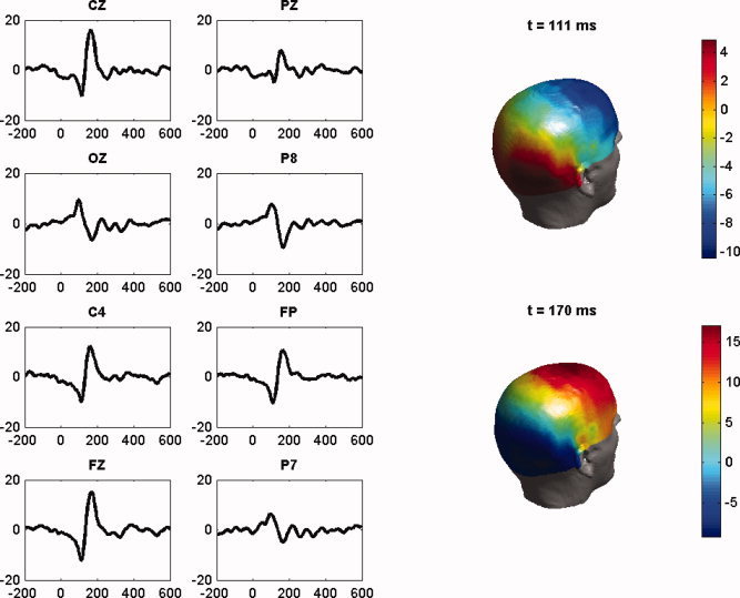
(a) Left: Average (over 76 trials) of the difference face—scrambled face EEG data for the channels CZ, PZ, IZ, P8, C4, FPZ, FZ, and P7, plotted against time t(ms). There is a negative EEG peak around t = 111 ms for the electrodes CZ, PZ, C4 in the temporal region, and FPZ and FZ in the frontal region, followed by a positive peak around 170 ms. The reverse happens in the occipito‐temporal channels OZ, P8, and P7 (the so‐called N170 component). (b) Right: the scalp topographic distribution of the 128 channels at the time instants t = 111 ms and t = 170 ms. [Color figure can be viewed in the online issue, which is available at www.interscience.wiley.com.]

As described in the previous section, our statistical tests assume the partition of the scalp channels into two disjoint subsets. That is, the raw data is partitioned in two data arrays [X]${}_{\mathit{\text{s,c}}{}_{\text{1}}\text{,τ}}$, c ₁ ∈ I ₁ and [X]${}_{\mathit{\text{s,c}}{}_{\text{2}}\text{,τ}}$, c ₂ ∈ I ₂, where in this example, I ₁ and I ₂ are sets of scalp channels corresponding to the left and right hemispheres, respectively. To remove the effect of familiar and unfamiliar faces depicted in Figure 1, we used the residuals obtained by subtracting the average of each group (familiar, unfamiliar) from the data in that group, to give S = 76−2 = 74 effectively independent observations.

Figure 2a shows the resulting greatest root statistic θ_t for t ∈ U = [−200,600] ms and the decision threshold at significance level α = 0.05 (dash vertical line) obtained by RFT as described in the previous section. For this analysis, just 11 spatially remote scalp channels (those shown in Fig. 2b) per hemisphere were selected. Notice the presence of several peaks of significant local maximum greatest root statistics. Our subsequent analysis focuses on the time intervals containing some significant instants marked with circles in the plot.

Figure 2.

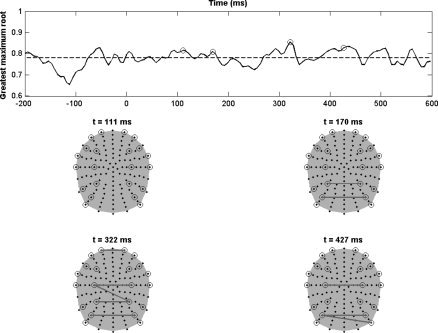
(a) Top: Greatest root statistics and decision threshold for an inter‐hemispheric comparison at significance level P = 0.05. (b) Bottom: Topographic maps of the correlation analysis at four different time instants of local maximum greatest maximum root statistics (marked with circle in the top plot). [Color figure can be viewed in the online issue, which is available at www.interscience.wiley.com.]

As expected, there is significant global connectivity between both hemispheres in the time interval [100,190] ms. However, some other interesting time intervals with significant values of greatest root statistics are [280,330] ms, [390,450] ms, and [480,510] ms. These findings seem to be related to the activity produced by the N170 component and certain significant activations at 300 ms, usually associated with a familiarity effect in the face recognition process [Henson et al., 2003].

The analysis of the topographic connectivity maps reveals no significant cross correlation at the time instant t = 111 ms. This seems to contradict Figure 2a, where significant global connectivity was detected at this time instant. This can be explained by the fact that the UI test is too conservative for detecting significant correlations associated with particular entries (Σ${}_{\text{12}}^{\mathit{\text{t}}}$)_ij. Recall that although UI tests are valid for hypothesis about any linear combination of the entries (Σ${}_{\text{12}}^{\mathit{\text{t}}}$)_ij, we only have considered here those linear combinations corresponding to hypotheses about each particular entry. On the other hand, there is a significant correlation in the topographic map corresponding to t = 170 ms, which should be associated with the bilateral occipital maximal negativity observed in Figure 1b. This result agrees with those of [Henson et al., 2003], where it a bilateral activation was reported in the occipital region around t = 170 ms, associated with a face perception process. Notice also a bilateral connectivity between occipital and temporal regions at t = 322 ms and t = 427 ms, as previously noted, related to a familiarity effect.

Tomographic connectivity maps at the four time instants 111 ms, 170 ms, 322 ms and 427 ms, are displayed in Figure 3. Notice that there exists a consistent significant homologous correlation in the right fronto‐temporal region, although this is extended to the right occipital region at time 170 ms. This fact suggests that such regions are involved in the face recognition process as sources that generate the selected scalp measurements in both hemispheres. This conclusion agrees with that reported in [Henson et al., 2003], where it was suggested that the brain activation produced by the face recognition process is mainly right lateralized. These results are also consistent with the classical cognitive “core model” for face recognition and perception [Gobbini and Haxby, 2007], because this cognitive process involves the processing and transfer of information in a neuronal network that includes brain structures in the occipital and frontal regions as well as in the superior‐temporal area.

Figure 3.

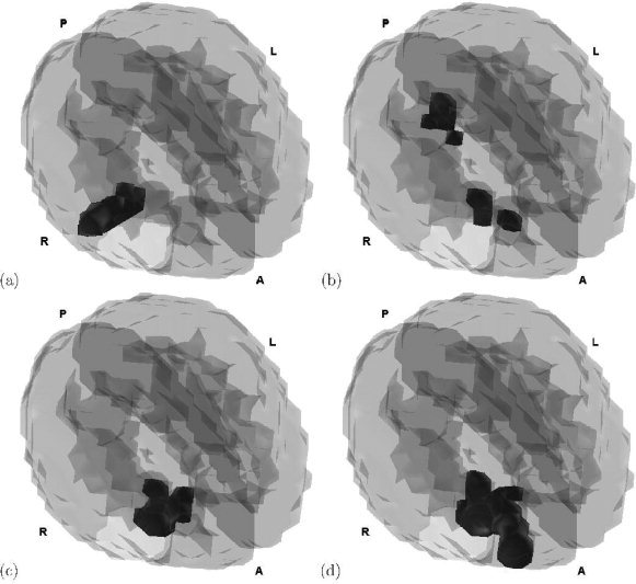
Tomographic maps of the homologous correlation analysis between the sources generated by the left and right scalp channels at times t = (a) 111 ms, (b) 170 ms, (c) 322 ms, (d) 427 ms. Letters A, P, L, R in each subplot mean anterior, posterior, left and right, respectively. We conclude that there are statistically significant homologous correlations mainly in the right fronto‐temporal region. [Color figure can be viewed in the online issue, which is available at www.interscience.wiley.com.]

DISCUSSION

In this section, we briefly present some extensions and some limitations of our proposed method. The exposition of our method is based on a connectivity analysis within a single EEG/MEG trial (condition) type. However, the whole analysis can be easily extended for comparison between two trial types. Indeed, the data array [X]${}_{\mathit{\text{s,c}}{}_{\text{1}}\text{,τ}}$, c ₁ ∈ I ₁ and [X]${}_{\mathit{\text{s,c}}{}_{\text{2}}\text{,τ}}$, c ₂ ∈ I ₂ could be considered as multivariate sample data matrices on two different trial types. Even more, they could also be considered as ERP/ERF data obtained from subjects under two different experimental conditions.

A possible limitation of the methods presented here is the basic model for the ERP/ERF as the linear superposition of the event related activity and background activity. This model is only a first approximation, useful for exploratory purposes. More realistic nonlinear and nonstationary models of the ERP/ERF may require more complex statistical procedures.

The extension of the test statistic to a whole time interval hinges on the use of RFT. As it was pointed out in [Taylor and Worsley, 2008], 2ρ_d(λ) is not the EC density of a Roy's maximum root random field, rather it is twice the alternating sum of the EC density of all roots. However, for high thresholds, the other roots are much smaller than the maximum and so their EC is close to zero. Some general underlying assumptions of RFT were already discussed in [Carbonell et al., 2004]. It should be also noted that, in contrast with classical connectivity analysis in 3D domains [Worsley et al., 1998], our approach here provides the same decision threshold G _α for homologous as well as for full cross‐correlations RFs. As we already mentioned, we restricted our analysis to 3D homologous random fields due to the high computational cost involved in the calculation of all 6D cross‐correlations.

CONCLUSIONS

A novel application of RFT and UI tests was introduced in the framework of EEG/MEG hypothesis‐testing problems. RFT was applied for solving the multiple comparisons problem that appears when examining the global null hypothesis of no temporal connectivity. On the other hand, UI tests were used for testing hypotheses about the topographic and tomographic distribution of the detected temporal connectivity between ERP/ERF components. Therefore, the combination of both techniques provided a general criterion for assessing simultaneously the spatio‐temporal detection of the correlation structure between ERP/ERF components as well as the time dependent cross‐correlation between its generating current density sources. Finally, physiologically meaningful results were obtained in the application of the statistical methodology to actual EEG data recorded from a face recognition experiment.

REFERENCES

- Astolfi L,Cincotti F,Mattia D,Marciani G,Baccala L,Fallani F,Salinari S,Ursino M,Zavaglia M,Ding L.Edgar JC,Miller GA,He B,Babiloni F ( 2007): Comparison of different cortical connectivity estimators for high‐resolution EEG recordings. Hum Brain Mapp 28: 143–157. [DOI] [PMC free article] [PubMed] [Google Scholar]
- Aunon JI,McGillen CD,Childers DC ( 1981): Signal processing in evoked potentials research: Averaging and modeling. CRC Crit Rev Bioeng 5: 323–367. [PubMed] [Google Scholar]
- Babiloni F,Cincotti F,Babiloni C,Carducci F,Mattia D,Astolfi L,Basilisco A,Rossini PM,Ding L,Ni Y,Cheng J,Christine K,Sweeney J,Heg B ( 2005): Estimation of the cortical functional connectivity with the multimodal integration of high‐resolution EEG and fMRI data by directed transfer function. NeuroImage 24: 118–131. [DOI] [PubMed] [Google Scholar]
- Baumgartner R,Ryner L,Richter W,Summers R,Jarmasz M,Somorjai R ( 2000): Comparison of two exploratory data analysis methods for fMRI: Fuzzy clustering vs. principal component analysis. J Magn Reson Imaging 18: 89–94. [DOI] [PubMed] [Google Scholar]
- Cao J,Worsley KJ ( 1999): The geometry of correlation fields with an application to functional connectivity of the brain. Ann Appl Probability 9: 1021–1057. [Google Scholar]
- Carbonell F,Galán L,Valdés P,Worsley KJ,Biscay RJ,Díaz‐Comas L,Bobes MA,Parra M ( 2004): Random Field‐union intersection tests for linear electrophysiological imaging. Neuroimage 22: 268–276. [DOI] [PubMed] [Google Scholar]
- Collins L,Neelin P,Peters TM,Evans AC ( 1994): Automatic 3D registration of MR volumetric data in standardized Talairach space. J Comput Assist Tomogr 18: 192–205. [PubMed] [Google Scholar]
- David O,Cosmelli D,Friston KJ ( 2004): Evaluation of different measures of functional connectivity using a neural mass model. Neuroimage 21: 659–673. [DOI] [PubMed] [Google Scholar]
- Evans AC,Collins DL,Mills SR,Brown ED,Kelly RL,Peters TM ( 1993): 3D Statistical Neuroanatomical Models from 305 MRI Volumes. Proceedings of IEEE‐Nuclear Science Symposium and Medical Imaging Conference 95. London: MTP Press. pp 192–205.
- Friston KJ ( 1996): Statistical parametric mapping and other analyses of functional imaging data In: Toga AW,Mazziotta JC, editors. Brain Mapping: The Methods. San Diego: Academic Press; pp 363–396. [Google Scholar]
- Friston KJ,Frith CD,Liddle PF,Frackowiak RS ( 1993): Functional connectivity: The principal‐component analysis of large (PET) data sets. J Cereb Blood Flow Metab 13: 5–14. [DOI] [PubMed] [Google Scholar]
- Gevins A ( 1989): Dynamic functional topography of cognitive task. Brain Topogr 2: 37–56. [DOI] [PubMed] [Google Scholar]
- Gevins A,Remond A ( 1987): Methods of analysis of brain electrical and magnetic signals Handbook of Electroencephalography and Clinical Neurophysiology,Vol. 1 Amsterdam: Elsevier. [Google Scholar]
- Gobbini MI,Haxby JV ( 2007): Neural systems for recognition of familiar faces. Neuropsychologia 45: 32–44. [DOI] [PubMed] [Google Scholar]
- Henson RN,Goshen‐Gottstein Y,Ganel T,Otten LJ,Quayle A,Rugg MD ( 2003): Electrophysiological and haemodynamic correlates of face perception, recognition and priming. Cereb Cortex 13: 793–805. [DOI] [PubMed] [Google Scholar]
- Hochberg Y,Tamhane AC ( 1987): Multiple Comparisons Procedures. New York: Wiley. [Google Scholar]
- Kaminski M,Ding M,Truccolo WA,Bressler S ( 2001): Evaluating causal relations in neural systems: Granger causality, directed transfer function and statistical assessment of significance. Biol Cybern 85: 145–157. [DOI] [PubMed] [Google Scholar]
- Kiebel S,Friston KJ ( 2004): Statistical parametric mapping for event‐related potentials: I. Generic considerations. NeuroImage 22: 492–502. [DOI] [PubMed] [Google Scholar]
- Koch MA,Norris DG,Hund‐Georgiadis M ( 2002): An investigation of functional and anatomical connectivity using magnetic resonance imaging. NeuroImage 16: 241–250. [DOI] [PubMed] [Google Scholar]
- Koenig T,Studer D,Hubl D,Melie L,Strik WK ( 2005): Brain connectivity at different time‐scales measured with EEG. Philos Trans R Soc B 360: 1015–1024. [DOI] [PMC free article] [PubMed] [Google Scholar]
- Kuhfeld W ( 1986): A note on Roy's largest root. Physchometrika 51: 479–481. [Google Scholar]
- Mardia KV,Kent JT,Bibby JM ( 1979): Multivariate Analysis. San Diego,California: Academic Press. [Google Scholar]
- Mazziotta JC,Toga A,Evans AC,Fox P,Lancaster J ( 1995): A probabilistic atlas of the human brain: Theory and rationale for its development. Neuroimage 2: 89–101. [DOI] [PubMed] [Google Scholar]
- Pascual‐Marqui RD,Esslen M,Kochi K,Lehmann D ( 2002): Functional imaging with low‐resolution brain electromagnetic tomography (LORETA): A review. Methods Find Exp Clin Pharmacol 24C: 91–95. [PubMed] [Google Scholar]
- Schindler K,Leung H,Elger CE,Lehnertz K ( 2007): Assessing seizure dynamics by analysing the correlation structure of multichannel intracranial EEG. Brain 130: 65–77. [DOI] [PubMed] [Google Scholar]
- Taylor JE,Worsley KJ ( 2008): Random fields of multivariate test statistics, with applications to shape analysis and fMRI. Ann Stat 37: 1–27. [Google Scholar]
- Thatcher RW,Biver CJ,North D ( 2007): Spatial‐temporal current source correlation and cortical connectivity. Clin EEG Neurosci 38: 35–48. [DOI] [PubMed] [Google Scholar]
- Trujillo‐Barreto N,Aubert‐Vazquez E,Valdés‐Sosa P ( 2004): Bayesian model averaging in EEG/MEG imaging. Neuroimage 21: 1300–1319. [DOI] [PubMed] [Google Scholar]
- Urbano A,Babiloni C,Onorati P,Babiloni F ( 1998): Dynamic functional coupling of high resolution EEG potentials related to unilateral internally triggered one‐digit movements. Electroencephalogr Clin Neurophysiol 106: 477–487. [DOI] [PubMed] [Google Scholar]
- van de Ven VG,Formisano E,Prvulovic D,Roeder CH,Linden DE ( 2004): Functional connectivity as revealed by spatial independent component analysis of fMRI measurements during rest. Hum Brain Mapp 22: 165–178. [DOI] [PMC free article] [PubMed] [Google Scholar]
- Worsley KJ,Cao J,Paus T,Petrides M,Evans AC ( 1998): Applications of random field theory to functional connectivity. Hum Brain Mapp 6: 364–367. [DOI] [PMC free article] [PubMed] [Google Scholar]
- Worsley KJ,Andermann M,Koulis T,MacDonald D,Evans AC ( 1999): Detecting changes in nonisotropic images. Hum Brain Mapp 8: 98–101. [DOI] [PMC free article] [PubMed] [Google Scholar]
- Worsley KJ,Taylor JE,Tomaiuolo F,Lerch J ( 2004): Unified univariate and multivariate random field theory. NeuroImage 23: S189–S195. [DOI] [PubMed] [Google Scholar]
- Worsley KJ,Chen J‐I,Lerch J,Evans AC ( 2005): Comparing connectivity via thresholding correlations and SVD. Philos Trans R Soc 360: 913–920. [DOI] [PMC free article] [PubMed] [Google Scholar]