Receptor architecture of human cingulate cortex: Evaluation of the four‐region neurobiological model

Abstract

The structural and functional organization of the human cingulate cortex is an ongoing focus; however, human imaging studies continue to use the century‐old Brodmann concept of a two region cingulate cortex. Recently, a four‐region neurobiological model was proposed based on structural, circuitry, and functional imaging observations. It encompasses the anterior cingulate, midcingulate, posterior cingulate, and retrosplenial cortices (ACC, MCC, PCC, and RSC, respectively). For the first time, this study performs multireceptor autoradiography of 15 neurotransmitter receptor ligands and multivariate statistics on human whole brain postmortem samples covering the entire cingulate cortex. We evaluated the validity of Brodmann's duality concept and of the four‐region model using a hierarchical clustering analysis of receptor binding according to the degree of similarity of each area's receptor architecture. We could not find support for Brodmann's dual cingulate concept, because the anterior part of his area 24 has significantly higher AMPA, kainate, GABA_B, benzodiazepine, and M₃ but lower NMDA and GABA_A binding site densities than the posterior part. The hierarchical clustering analysis distinguished ACC, MCC, PCC, and RSC as independent regions. The ACC has highest AMPA, kainate, α₂, 5‐HT_1A, and D₁ but lowest GABA_A densities. The MCC has lowest AMPA, kainate, α₂, and D₁ densities. Area 25 in ACC is similar in receptor‐architecture to MCC, particularly the NMDA, GABA_A, GABA_B, and M₂ receptors. The PCC and RSC differ in the higher M₁ and α₁ but lower M₃ densities of PCC. Thus, multireceptor autoradiography supports the four‐region neurobiological model of the cingulate cortex. Hum Brain Mapp, 2009. © 2008 Wiley‐Liss, Inc.

INTRODUCTION

The human cingulate cortex has been the subject of research for over a century. And yet, its structural and functional organization remains subject to debate. The cingulate gyrus forms a continuous structure along the mesial surface of the brain and was originally described as “le grand lobe limbique,” a region thought to be involved in emotion [Broca,1878; MacLean,1990; Papez,1937]. Brodmann [1909] was the first to propose the concept of a rostrocaudal cingulate dichotomy of the cingulate gyrus. Based on cytoarchitectonical observations, he defined a precingulate subregion, which spans the rostral portion of the cingulate gyrus, and a postcingulate subregion. The precingulate subregion contains areas 24, 25, 32, and 33 and is mainly agranular in nature (although area 32 has a thin, dysgranular layer IV), whereas the postcingulate subregion encompasses areas 23 and 31 and exhibits a prominent layer IV.

In recent decades, Brodmann's [1909] precingulate subregion was shown to be structurally and functionally inhomogeneous [Braak,1976; Phan et al.,2002; Vogt and Pandya,1987; Vogt et al.,2005; Whalen et al.,1998], and was, therefore, subdivided into two qualitatively distinct regions [Vogt and Vogt,2003]: the anterior cingulate cortex (ACC, the rostral portion of Brodmann's precingulate subregion) and the midcingulate cortex (MCC, the caudal portion of Brodmann's precingulate subregion). Structurally, MCC is characterized by large, neurofilament‐expressing neurons in layer IIIc and the presence of large layer Vb pyramidal neurons that are not found in other parts of the cingulate cortex [Braak,1976; Vogt and Vogt,2003; Vogt et al.,2003,2005]. In monkeys ACC is reciprocally connected with the amygdala, whereas MCC receives major projections from the parietal lobe but only has a modest amygdalar input, which is restricted to its most rostral part [Vogt and Pandya,1987]. ACC receives projections from areas 9 and 10, whereas MCC receives area 11 efferents [Petrides and Pandya,2007]. Additionally, MCC contains the cingulate motor areas, which project directly to the spinal cord [Dum and Strick,1993]. Functionally, the ACC primarily subserves emotion and is involved in visceromotor and endocrine control, whereas MCC is involved in skeletomotor control including pain processing [Vogt,2005]. Thus, MCC is not just a caudal subdivision of ACC, but shows fundamental differences that enable its definition as a qualitatively unique region.

The ACC can be further subdivided into a subgenual (sACC, below the genu of the corpus callosum) and a pregenual (pACC, rostral and dorsal to the genu) subregion [Gittins and Harrison,2004; Palomero‐Gallagher et al.,2008]. The sACC encompasses not only area 25, but also the most ventral portions of areas 24, 32, and 33. Subgenual components of areas 24 and 32 have a thinner cortex and a lower glia to neuron ratio than their pregenual counterparts [Gittins and Harrison,2004]. Subgenual area 24 has a thinner layer III than its pregenual counterpart, and layer II in subgenual 32 is of particular note because it has a neuron dense layer IIa and sparse layer IIb [Palomero‐Gallagher et al.,2008]. Electrical stimulation studies have shown that sACC is involved in the inhibition of autonomic responses via activation of area 25 [Burns and Wyss,1985], whereas stimulation of area 32 results in increased blood pressure [Fernandes et al.,2003]. Behavioral provocation of intense sadness is associated with acute focal increases in sACC blood flow [Mayberg et al.,1999]. Thus, the involvement of sACC in affective and autonomic responses would occur via the projections of areas 25 and 32 to autonomic motor nuclei in the brainstem such as the periaqueductal gray [An et al.,1998; Chiba et al.,2001; Freedman et al.,2000; Neafsey et al.,1993]. The pACC is involved in conditioned emotional learning, vocalizations associated with expressing internal states, assessments of motivational content, and assigning emotional valence to internal and external stimuli [Phan et al.,2002; Pool and Ransohoff,1949; Talairach et al.,1973; Vogt,2005; Vogt et al.,2003].

The MCC has been further subdivided into an anterior (aMCC) and a posterior (pMCC) subregion [Vogt et al.,2003]. It mediates motor/cognitive processes via premotor planning with motivational characteristics [Bush et al.,2002], functions which are implemented through the cingulospinal projections that arise from the cingulate motor areas [Strick et al.,1998]. From the cytological point of view, layer III is less differentiated and contains less neurofilament protein‐expressing neurons in aMCC, whereas layer Va is much more cell dense in pMCC [Vogt and Vogt,2003; Vogt et al.,2003,2005]. The amygdala projects modestly to aMCC, but not to pMCC [Vogt and Pandya,1987]. The aMCC contains part of the rostral cingulate motor area, is active during fear, and plays a larger role in the reward coding of behavior, whereas pMCC contains part of the caudal cingulate motor area and does not appear to be activated by simple emotions, but is more easily driven by passive movements [Meyer et al.,1973; Shima and Tanji,1998; Shima et al.,1991].

Two regions have been defined within the cingulate cortex located caudal to MCC: the posterior cingulate (PCC) and the retrosplenial (RSC) cortices. The PCC corresponds to Brodmann's [1909] postcingulate subregion, encompasses areas 23 and 31, and is involved in spatial orientation [Olson et al.,1996; Sugiura et al.,2005]. It has been further subdivided into the dorsal (dPCC, areas 23d and d23) and ventral (vPCC, area v23) subregions based on structural, connectivity, and functional considerations. Layers II, III, and V of vPCC are denser and contain larger pyramids than those of dPCC [Vogt et al.,2005,2006]. Additionally, layer III of vPCC is considerably thicker and contains a substantially higher density of neurofilament protein immunoreactive neurons than that of dPCC [Vogt et al.,2005]. Hodological studies in monkeys have shown that dPCC receives afferents from the dorsal bank of the principal sulcus, whereas cortex in the rostral tip of both banks projects to vPCC [Vogt and Barbas,1988]. Additionally, vPCC has reciprocal connections with subgenual ACC [Vogt and Pandya,1987] and receives efferents from medial area 9 [Petrides and Pandya,2007]. dPCC, but not vPCC, receives inputs from the central laterocellular, mediodorsal, as well as ventral anterior and ventral lateral thalamic nuclei [Shibata and Yukie,2003]. Functionally, dPCC has been implicated in visuospatial processing and body orientation in space and plays a role in polymodal stimulus‐response mapping, whereas vPCC is involved in the assessment of the self‐relevance of sensory events and their contexts [Ferstl and von Cramon,2007; O'Hare et al.,2008; Sugiura et al.,2005; Vogt et al.,2006].

The RSC, which comprises proisocortical areas 29 and 30, underlies memory and visuospatial functions [Burgess,2008; Iaria et al.,2007; Keene and Bucci,2008; Parker and Gaffan,1997; Vogt and Laureys,2005; Vogt et al.,1987,2001]. Although Brodmann [1909] described RSC as being restricted to the most caudal portion of the cingulate gyrus directly behind the splenium, more recent studies [Kobayashi and Amaral,2000; Vogt et al.,2001,2004] have shown that it extends further dorsally and rostrally along the callosal sulcus. Thus, the first undifferentiated parts of areas 29 and 30 can be seen at the level of PCC area 23d. Area 29 is characterized by a dense granular layer, can be subdivided into lateral and medial parts and is buried within the callosal sulcus, whereas area 30 encroaches onto the surface of the cingulate gyrus and is dysgranular [Vogt et al.,2001].

The combined results of these findings led to the proposal of a four‐region neurobiological model [Vogt et al.,2003,2006] that integrates structural, circuitry, and functional organization and comprises the ACC, MCC, PCC, and RSC regions. The primary difference with the Brodmann [1909] view is that MCC is not just seen as a caudal subdivision of ACC, but shows fundamental differences which enable its classification as a qualitatively unique region. Likewise, the four‐region neurobiological model disputes the terms “rostral” and “caudal” ACC, which are commonly employed in functional imaging studies to designate the location of activation sites within Brodmann's precingulate subregion [e.g., Botvinick et al.,2004; Davis et al.,2005; Grabenhorst et al.,2007; Holroyd and Coles,2008; Margulies et al.,2007], because they imply that these are fundamentally the same region and fail to integrate a much wider set of observations.

Receptors for classical neurotransmitters are heterogeneously distributed throughout the cerebral cortex [Zilles et al.,2002a] and provide a new approach to analyzing cingulate organization. Interareal borders revealed by the neurochemical structure of the cerebral cortex coincide with cytoarchitectonical parcellations and reflect the functional organization of the brain [Zilles et al.,2004]. Because receptors have pre‐ and postsynaptic links in specific circuits, they tend to reflect variations in circuitry and function and could provide independent verification of earlier cytological and connectional observations in the cingulate cortex. Examples of how receptor groupings have been used to study the primate cerebral cortex are available in visual [Eickhoff et al.,2007, in press; Rakic et al.,1988; Zilles and Clarke,1997], motor [Geyer et al.,1996,1998; Lidow et al.,1989], somatosensory [Lidow et al.,1989], auditory [Morosan et al.,2004], prefrontal [Goldman‐Rakic et al.,1990], cingulate [Bozkurt et al.,2005], and parietal [Scheperjans et al.,2005a,b] cortices.

Recent studies have generally employed 15 receptors for classical neurotransmitters for which tritiated, high‐affinity ligands are available. The complex codistribution patterns of various receptors in architectonically defined brain regions stimulated the introduction of a new analytical procedure, the receptor fingerprint [Zilles and Palomero‐Gallagher,2001], which is a polar coordinate plot showing the mean regional densities of several different receptors over all cortical layers in a single, architectonically defined brain region. In this framework, therefore, the multivariate analysis of 15 receptors provides a marker for the unique organization of different cortical areas, and a hierarchical cluster analysis has been used to integrate information from the multiple transmitter receptor systems and reveal segregation of cortical areas in the human superior parietal cortex based on their relations to regions involved in visual and somatosensory processing [Scheperjans et al.,2005b].

In this study, we first explore the extent to which the anterior and posterior parts of Brodmann's area 24 differ in their chemical organization. The null hypothesis states that no differences should exist if this is a uniform region as often assumed. Because the null hypothesis was rejected, we next evaluated the four‐region neurobiological model with a multivariate assessment of patterns of neurotransmitter receptor binding. Finally, all cingulate areas and regions are considered individually as defined in the four‐region model. For the first time, this study reports the mean regional densities of single and multiple groups of receptors in characterizing cingulate areas, subregions, and regions. Explicit proof is generated confirming that MCC is qualitatively different from ACC.

MATERIALS AND METHODS

We examined four brains obtained with a postmortem delay of 8–13 h from patients with no record of neurological or psychiatric diseases (age between 67 and 77 years; 3 males, 1 female). Brains were cut into slabs (2‐ to 3‐cm thick) at autopsy, frozen in isopentane at −40°C, and stored in airtight bags at −80°C. All subjects had given written consent before death and/or had been included in the body donor program of the Department of Anatomy, University of Düsseldorf, Germany.

Serial coronal sections were cut 20‐μm thick using a large‐scale cryostat microtome and adjacent glass‐mounted sections were processed for quantitative in vitro receptor autoradiography and for a cell‐body histological staining [Merker,1983]. We examined the laminar and regional distribution patterns of 15 receptors for the classical neurotransmitters glutamate (AMPA, kainate, and NMDA receptors), GABA (GABA_A and GABA_B receptors, GABA_A associated benzodiazepine [BZ] binding sites), acetylcholine (muscarinic M₁, M₂, and M₃ as well as nicotinic receptors), noradrenaline (α₁ and α₂ receptors), serotonin (5‐HT_1A and 5‐HT₂ receptors), and dopamine (D₁ receptors).

Labeling of receptor binding sites was carried out according to standard procedures for receptor autoradiography summarized in Table I [Zilles et al.,2002a,b], which involve three steps: a preincubation, a main incubation, and a final rinsing. The aim of the preincubation is the rehydration of sections and removal of endogenous substances which bind to the examined receptor and thus block the binding site for the tritiated ligand. In the main incubation, adjacent sections are incubated in a buffer solution containing either a tritiated ligand, or the tritiated ligand plus a nonlabeled specific displacer. Incubation of brain sections with a labeled ligand alone demonstrates the total binding of this ligand, and incubation with the tritiated ligand in the presence of a specific displacer is necessary to determine what proportion of the total binding sites is occupied by nonspecific, and thus nondisplaceable binding. Specific binding is the difference between total and nonspecific binding. Nonspecific binding in this study was less than 5% of total binding; thus, total binding closely reflects specific binding. Radioactively labeled sections were then coexposed with plastic standards of known radioactivity concentrations (Microscales®, Amersham) against tritium‐sensitive films (Hyperfilm, Amersham, Braunschweig, Germany) for 4–18 weeks.

Table I.

Summary of incubation conditions for receptor autoradiography

Transmitter	Receptor	[3H]‐Ligand	Displacer	Incubation buffer	Preincubation	Main incubation	Rinsing
Glutamate	AMPA	AMPA [10 nM]	Quisqualate [10 μM]	50 mM Tris‐acetate (pH7.2) + 100 mM KSCN (M)	3 × 10 min at 4°C	45 min at 4°C	4 × 4 s in buffer at 4°C
							2 × 2 s fixationa at 4°C
	Kainate	Kainate [8 nM]	Kainate [100 μM]	50 mM Tris‐citrate (pH7.1) + 10 mM Ca‐acetate (M)	3 × 10 min at 4°C	45 min at 4°C	4 × 4 s in buffer at 4°C
							2 × 2 s in fixationa at 4°C
	NMDA	MK‐801 [5 nM]	(+) MK‐801 [100 μM]	50 mM Tris‐HCl (pH7.2) + 30 μM Glycine (M) + 50 μM Spermidine (M)	15 min at 22°C	60 min at 22°C	2 × 5 min in buffer at 4°C
							2 dips in distilled H2O
GABA	GABAA	Muscimol [3 nM]	GABA [10 μM]	50 mM Tris‐citrate (pH7.0)	3 × 5 min at 4°C	40 min at 4°C	3 × 3 s in buffer at 4°C
							2 dips in distilled H2O
	GABAB	CGP 54626 [1.5 nM]	CGP 55845 [100 μM]	50 mM Tris‐HCl (pH 7.2) + 2.5 mM CaCl2	3 × 5 min at 4°C	60 min at 4°C	3 × 2 s in buffer at 4°C
							2 dips in distilled H2O
	BZ	Flumazenil [0.8 nM]	Clonazepam [2 μM]	170 mM Tris‐HCl (pH 7.4)	15 min at 4°C	60 min at 4°C	2 × 1 min in buffer at 4°C
							2 dips in distilled H2O
Acetylcholine	M1	Pirenzepine [1 nM]	Pirenzepine [10 μM]	modified Krebs‐Ringer Buffer (pH7.4)	20 min at 22°C	60 min at 22°C	2 × 5 min in buffer at 4°C
							2 dips in distilled H2O
	M2	Oxotremorine‐M; [0.8 nM]	Carbachol [1 μM]	20 mM Hepes‐Tris (pH7.5) + 10 mM MgCl2	20 min at 22°C	60 min at 22°C	2 × 2 min in buffer at 4°C
							2 dips in distilled H2O
	M3	4‐DAMP [1 nM]	Atropinsulfate [10 μM]	20 mM Tris‐HCl (pH7.4) + 1 mM PSMF + 1 mM EDTA	15 min at 22°C	45 min at 22°C	2 × 5 min in buffer at 4°C
							2 dips in distilled H2O
	N	Epibatidine [0.5 nM]	Nicotine‐di‐ hydrogen‐tartrate [100 μM]	15 mM Hepes‐Tris (pH7.5) + 120 mM NaCl + 5.4 mM KCl + 0.8 mM MgCl2 + 1.8 mM CaCl2	20 min at 22°C	90 min at 22°C	5 min in buffer at 4°C
							2 dips in distilled H2O
Noradrenaline	α1	Prazosin [0.2 nM]	Phentolamine [10 μM]	50 mM Tris‐HCl (pH7.4)	30 min at 37°C	45 min at 30°C	2 × 5 min in buffer at 4°C
							2 dips in distilled H2O
	α2	RX‐821002 [6 nM]	(−)adrenalin [10 μM]	50 mM Tris‐HCl (pH7.4) + 1 mM MgCl2 + 0.1% ascorbic acid + 0.3 μM 8‐OH‐DPAT (M)	30 min at 22°C	30 min at 22°C	2 × 20s in buffer at 4°C
							2 dips in distilled H2O
Serotonin	5‐HT1A	8‐OH‐DPAT [1 nM]	Serotonin [10 μM]	170 mM Tris‐HCl (pH7.6) + 4 mM CaCl2 + 0.01% Ascorbic acid	30 min at 22°C	60 min at 22°C	1 × 5 min in buffer at 4°C
							2 × dips in distilled H2O
	5‐HT2	Ketanserine [0.5 nM]	Mianserine [10 μM]	170 mM Tris‐HCl (pH7.7)	30 min at 22°C	120 min at 22°C	2 × 10 min in buffer at 4°C
							2 × dips in distilled H2O
Dopamine	D1	SCH‐23390 [0.5 nM]	SKF 83566 [1 μM]	50 mM Tris‐HCl (pH 7.4) + 120 mM NaCl + 5 mM KCl + 2 mM CaCl2 + 1 mM MgCl2 + 1 μM mianserin (M)	20 min at 22°C	90 min at 22°C	2 × 10 min in buffer at 4°C
							2 × dips in distilled H2O

(M), substances added to buffer only during the main incubation.

^aFixation in a 100 ml/2.5 ml acetone/glutaraldehyde solution.

The resulting autoradiographs were processed by densitometry [Zilles et al.,2002b]. In short, autoradiographs were digitized by means of a KS‐400 image analyzing system (Kontron, Germany) and a digital camera (ProgRes C14, Zeiss Jena, Germany) with a resolution of 2600 × 2060 pixels and 8‐bit gray resolution, as exemplarily shown in Figure 1A. Because these images only code gray values, and not concentrations of radioactivity, a scaling was carried out, in which the gray values were transformed into fmol binding sites/mg protein. This scaling was performed in two stages [Zilles et al.,2002b]: (i) The gray value images of the coexposed Microscales® were used to compute a calibration curve, which defined the nonlinear relationship between gray values in the autoradiographs and concentrations of radioactivity. (ii) This concentration of radioactivity (R) was subsequently converted to a binding site density (C _b) using the following equation:

where E is the efficiency of the scintillation counter used to determine the amount of radioactivity in the incubation buffer, B is the number of decays per unit of time and radioactivity, W _b is the protein weight of a standard, S _a is the specific activity of the ligand, K _D is the dissociation constant of the ligand, and L is the free concentration of the ligand during incubation. The result of this correction was a linearized image (Fig. 1B) in which each pixel codes for a receptor density in fmol/mg protein.

Figure 1.

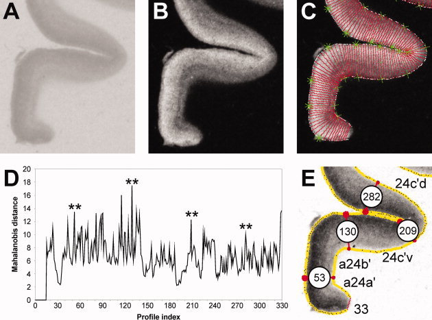
Summary of the algorithm‐based observer interactive method applied to determine cortical borders. A. Digitized autoradiograph of a coronal section through the cingulate gyrus in which the M ₁ receptors were labeled with [³H]pirenzepine. B. Linearized image shown in A. C. Two contour lines (white) define the cortical region to be sampled in the image shown in B by profiles spanning the ribbon. The outer contour marks the pial surface, the inner contour the layer VI/white matter border. Each of the equidistant traverses (red lines) marks the location of a profile. The green symbols indicate the start (asterisks) and end (crosses) points of every tenth profile. D. Distance analysis based on profiles indicated in C. Asterisks highlight main maxima with significant P values (P < 0.01, interareal borders) at positions 53, 130, 209, and 282. E. Result of the algorithm‐based border detection applied to the section shown in A. Red lines highlight the profile identified by the distance analysis as an interareal border and numbers in the white circles indicate the number of the profile in question. Thus, profile 53 defines the border between areas a24a′ and a24b′; profile 130 that between areas a24b′ and 24c′v; profile 209 that between areas 24c′v and 24c′d; profile 282 that between areas 24c′d and 32′.

Cortical borders were identified by means of an observer interactive approach based on the quantification of the neocortical laminar pattern by defining intensity line profiles across the cortical layers. Determination of the regions of interest from which profiles were to be extracted was based on macroscopical brain landmarks and Brodmann's maps [1909]. For example, we expected to find Brodmann's areas 24 and 23 on the cingulate gyrus, and areas 29, 30, and 33 within the callosal sulcus. Thus, profiles were extracted from sections equidistantly spaced along the rostrocaudal axis of the cingulate cortex between the paracingulate and the parieto‐occipital sulci and covered the cingulate and superior cingulate gyri as well as the parasplenial lobules. Furthermore, autoradiographs were compared with neighboring cell‐body stained sections and areas were anatomically identified based on criteria described for existing cingulate parcellation schemes, in particular those of Brodmann [1909] and Vogt and coworkers [Vogt and Vogt,2003; Vogt et al.,1995,2001,2003,2004]. Therefore, an area located on the cingulate gyrus was considered as being part of area 24 if analysis of the neighboring histological section revealed an agranular cortex, whereas it was classified as being part of area 23 if layer IV was present.

Equidistant intensity profiles oriented vertically to the cortical surface (Fig. 1C) were extracted by means of a minimum length algorithm from the digitized and linearized autoradiographs [Schleicher et al.,2000]. Receptor‐profiles quantify the laminar receptor density (in fmol/mg protein) from the pial surface to the border between layer VI and the white matter. The shape of a profile can be expressed by a vector of 10 features based on central moments (mean receptor density, mean x, SD, skewness and kurtosis, as well as the analogous parameters from the absolute values of its first derivative). Differences between feature vectors indicate differences in the shape of the profiles (which reflect receptor‐architecture), and were measured by means of the Mahalanobis distance. The set of profiles extracted from each image was analyzed for areal borders using a sliding window procedure, under the assumption that each area reveals a unique, homogeneous laminar pattern. To increase the signal‐to‐noise ratio, distances were calculated between feature vectors from blocks of n (10 < n < 34) adjacent profiles and were analyzed as a function of the profile number between the blocks. The resulting distance function revealed maxima (i.e., borders; Fig. 1D), at those positions at which the laminar patterns of the areas covered by the two blocks of profiles differed most and the significance of these maxima was evaluated by a Hotelling's T ²‐test with a Bonferroni‐correction for multiple comparisons (P ≤ 0.01).

Although each receptor does not indicate all areal borders, there is a perfect agreement in the location of those borders, which are displayed by several receptors [Zilles et al.,2004]. The superposition of all borders revealed by all examined receptor types yielded the parcellation scheme of the cingulate cortex based on its receptor architecture. For each brain, area, and receptor type, profiles extracted from three to five sections were averaged and the surface defined beneath the ensuing mean profile was computed to yield the absolute binding site densities for the entire cortical depth in that particular area. This value will be subsequently referred to as “mean density.”

We evaluated binding in the anterior and posterior parts of Brodmann's area 24 to determine whether the examined receptors are heterogeneously distributed throughout its rostrocaudal axis. This was done by means of an index (AI_a/p) quantifying the asymmetry between the anterior and posterior portions of area 24, which was computed for each receptor type according to the following equation:

where A _a is the concentration of the receptor in question averaged over the sections covering the rostral third of area 24 and A _p is the concentration of the receptor in question averaged over the sections covering the caudal two‐thirds of area 24. We subsequently applied one‐sample t‐tests to determine for each receptor type whether its AI_a/p differed significantly from 0 (expected value). Positive AI_a/p values reflect higher receptor densities in the anterior than in the posterior portion of area 24, whereas the opposite holds true for negative AI_a/p values. Significance level was set at P ≤ 0.01.

Receptors were evaluated for a possible heterogeneous distribution throughout the entire cingulate cortex by means of an ANOVA with repeated measures (P < 0.01). This was followed by one‐sample t‐tests (P < 0.01), which were carried out for those receptor types found to be heterogeneously distributed throughout the cingulate cortex to determine which area contributed to the significance. Additionally, we assessed which isocortical areas of ACC differed significantly in their mean densities from area 25, because this area clustered with areas in aMCC although we predicted a clustering with the remaining areas of ACC (pACC, see Results and Discussion). The ANOVA with repeated measures (P < 0.01) was followed by one‐sample t‐tests (P < 0.05) in which the mean density of a given receptor in areas 24a, 24b, 24c, or 32 was compared with the mean density (averaged over all brains) of that receptor in area 25.

Hierarchical clustering analyses were conducted to detect putative groupings of cingulate areas according to the degree of similarity of receptor‐architecture using Matlab Statistics Toolbox (MatLab 7.1; Mathworks, Natick, MA). In the hierarchical cluster analysis, a set of cortical areas is grouped into clusters in such a way that areas in the same cluster are similar with respect to their receptor‐architecture, and different from areas in other clusters. We applied the Euclidean distance as a measure of (dis)similarity because it takes both differences in the size and in the shape of receptor fingerprints into account, and the Ward linkage algorithm as the linkage method. This combination yielded the maximum cophenetic correlation coefficient as compared to any combination of alternative linkage methods and measurements of (dis)similarity. The cophenetic correlation coefficient quantifies how well a dendrogram represents the true, multidimensional distances within input data.

Receptor densities were normalized before carrying out multivariate statistical tests by dividing the mean density of each subregion by the grand mean of the receptors, that is, the average of mean densities of this receptor across all subregions under investigation. This normalization has two advantages: (i) because the absolute levels of receptor densities vary considerably among receptors (28 fmol/mg protein, nicotinic receptors; 3,195 fmol/mg protein, BZ binding sites), normalization assigns equal weight to each receptor. Without normalization, receptors exhibiting high absolute density levels would dominate the calculation of the Euclidean distance between areas, thus introducing a bias. (ii) Normalization as performed does not rule out the differences in receptor densities among subregions. The relative differences are preserved and are used as a valuable parameter in multivariate statistics such as hierarchical cluster analysis.

RESULTS

Receptor Analysis of the Brodmann Model

The null hypothesis states that Brodmann's area 24 is a functionally uniform area, neurotransmitter receptor binding reflects a neurochemical uniformity and that the MCC does not exist. Figure 2A presents Brodmann's map of cingulate areas coregistered to the medial surface of a post‐mortem case and this coregistration was used to assess binding in each of Brodmann's areas. The hierarchical analysis is shown in Figure 2B and reveals that Brodmann's areas from anterior, posterior, and retrosplenial cortices are associated as predicted; that is, areas in similar regions have similar binding patterns. However, for this analysis to be correct, it must be shown that binding within all areas is homogeneous and that the regions and their further subdivisions as proposed in the four‐region model are not justified.

Figure 2.

The cingulate cortex as defined by Brodmann [1909]. A. Schematic drawing showing the regions, subregions and areas defined by Brodmann within the human cingulate cortex. The precingulate subregion encompasses areas 33, 25, 24, and 32; the postcingulate subregion areas 23 and 31; the retrosplenial region areas 29 and 30. The callosal (cas), cingulate (cgs), paracingulate (pcgs), and splenial (spls) sulci were “opened” to show areas within them. B. Result of the hierarchical clustering of cingulate regions defined by Brodmann based on their neurochemical structure. The length of the branches indicates the degree of (dis)similarity between the joined clusters. The shorter the branch, the more similar two elements or groups of elements are. The mean receptor densities of area 24 used in this analysis were obtained by averaging all profiles located between white lines in C. C. Coronal sections through two different rostrocaudal levels of area 24 showing the distribution of the GABA_A (top row) and AMPA (bottom row) receptors. Lines indicate the position of borders detected by the algorithm‐based quantification of cortical receptor profiles. White lines indicate the borders of area 24 as defined by Brodmann. Black lines highlight borders detected within Brodmann's area 24. The lines are continuous when the receptor in question reveals the border and dotted when the border is revealed by other receptors (for example, receptors shown in Levels 1 [anterior 24] and 3 [posterior 24] of Fig. 3B). Colour scales code receptor densities in fmol/mg protein. D. Heterogeneous distribution of receptors throughout the rostrocaudal axis of area 24 as revealed by the asymmetry index (AI_a/p). The mean receptor densities used in this analysis were obtained by averaging all profiles located between white lines in C and extracted from sections covering the rostral third (A _a value) or the caudal two thirds (A _p) of area 24. Positive AI_a/p values indicate higher densities of the receptor in question in the rostral than in the caudal third of area 24. An AI_a/p of 0 (expected value) indicates a homogeneous receptor distribution. Asterisks indicate those receptors for which AI_a/p values differ significantly (P ≤ 0.01) from 0.

A visual review of binding in area 24 shows that the anterior and posterior parts of this area are not the same. The border between the anterior and posterior area 24 is marked with an arrowhead in Figure 2A and examples of binding for two transmitter systems in both parts of area 24 are shown in Figure 2C. The GABA_A receptors are in lower densities in the anterior than in the posterior portion of area 24, as clearly revealed by the colour scale; the superficial layers of anterior area 24 are coded in yellow and pale orange (mean receptor density of 663 ± 129 fmol/mg protein), whereas red is the predominant colour in posterior area 24 (mean receptor density of 1,227 ± 29 fmol/mg protein). In contrast, the AMPA receptors present the opposite situation with higher densities in the anterior than the posterior portions of area 24 (Fig. 2C); the predominant colors in anterior area 24 are red and orange tones (mean receptor density of 582 ± 152 fmol/mg protein), whereas green and blue are the predominant colors in posterior area 24 (mean receptor density of 336 ± 87 fmol/mg protein). The following question arises from these observations: Are these variations reflected in statistical differences for many receptors and might this information force a rejection of the null hypothesis?

To quantitatively evaluate the anterior/posterior area 24 differences for all receptors, the AI_a/p ratio was calculated for each receptor as shown in Figure 2D. Eight receptors had binding that differed significantly from AI_a/p = 0. The one‐sample t‐tests revealed that AI_a/p values of NMDA and GABA_A receptors, which were negative (Fig. 2D), differed significantly from the expected value (0, P ≤ 0.01). Similarly, the AI_a/p ratios of AMPA, kainate, GABA_B, M₃, and D₁ receptors as well as of BZ binding sites (Fig. 2D), which were positive, differed significantly from 0 (P ≤ 0.01). In view of the differences in receptor binding for anterior/posterior area 24, we must reject the null hypothesis and thus confirm the definition of the ACC and MCC regions based on differences in mean receptor densities. A prime is used to identify caudal area 24: area 24 is in ACC, whereas area 24′ is in MCC. Therefore, from here on, binding will be evaluated in terms of the recent definition of ACC [Palomero‐Gallagher et al.,2008] and the four‐region model with the dichotomies expressed in ACC, MCC, and PCC.

Receptor Analysis of Area Borders in the Four‐Region Model

Receptors for classical neurotransmitters are heterogeneously distributed throughout the human cingulate cortex. The algorithm‐based quantification of interareal differences in regional and laminar receptor distribution patterns revealed that although a given receptor type does not necessarily indicate all areal borders, there is a very close agreement in the location of those borders when displayed by several receptors. The superposition of all borders revealed by all examined receptor types yielded the parcellation scheme of the cingulate cortex based on its receptor architecture and is schematically shown in Figure 3A. Anatomical identification of these areas and regions was carried out by comparing our cell‐body stained sections with existing descriptions according to the four‐region model of cingulate cortex.

Figure 3.

A. The four‐region neurobiological model and cytoarchitectural areas [Vogt et al.,2004]. The callosal, cingulate (cgs), paracingulate (pcgs) and splenial sulci were “opened” to show areas within them. The ACC areas (33, 25, 24a, 24b, 24cv, 24cd, and 32) are coded in red; MCC areas (33, a24a′, a24b′, a24c′v, a24c′d, p24a′, p24b′, 24dv, 24dd) in green; PCC areas (23d, 23c, d23, v23, 31) in blue; and RSC areas (29l, 29m, 30) in gray. Arrowheads mark the four levels at which autoradiographs shown below were obtained. B. Exemplary autoradiographs through four rostrocaudal levels of the human cingulate gyrus. Lines indicate the position of borders detected by the algorithm‐based quantification of cortical receptor profiles. The lines are continuous when the receptor in question reveals the border and dotted when the border is revealed by other receptors. Note, that layer I is partially missing in area 24b, as clearly shown by the α₁ receptors (B₁: top row of autoradiographs).

Subdivisions of area 24

Distribution patterns of receptor binding not only revealed differences throughout the rostrocaudal axis of area 24, but also confirmed the existence of subdivisions along its dorsoventral axis. In the rostrocaudal dimension, we distinguish areas 24 (ACC), a24′ (anterior subdivision of MCC), and p24′ (posterior subdivision of MCC). Dorsoventrally, there are three divisions of area 24 based on progressively increasing laminar differentiation: a (located next to area 33), b, and c/d. As described in detail below, only some of the examined receptors reveal all subdivisions of area 24.

The algorithm‐based quantification of receptor profiles also confirmed the recently described subdivision of area 24c [Palomero‐Gallagher et al.,2008] and enabled the definition of a hitherto unknown border within area 24c′ (Figs. 1E and 3B). Each of these areas can be subdivided into a portion located on the ventral wall of the cingulate sulcus (24cv and 24c′v) and a portion restricted to the dorsal wall of the cingulate sulcus (24cd and 24c′d). Area 24cv contains higher AMPA, kainate, M₁, α₁, and D₁ but lower BZ and α₂ binding site densities than area 24cd (Fig. 3B). Area 24c′v contains higher kainate, NMDA, GABA_B, M₁, M₂, α₁, and D₁ but lower AMPA and α₂ receptor densities than area 24c′d (Figs. 1E and 3B).

Subdivisions of area 32

Using the algorithm‐based quantification of receptor profiles, it was confirmed that area 32 is not uniform in terms of receptor binding. This area has a rostral area 32 located over area 24 and a caudal area 32′ which extends over area a24′. Area 32 contains higher GABA_B, BZ, M₁, and 5‐HT_1A but lower NMDA and GABA_A binding site densities than area 32′.

Subdivisions of area 23

The heterogeneous distribution of receptors throughout area 23 enabled the definition of areas 23d, 23c, d23, and v23 as shown in Figure 3A. The borders between these areas were confirmed with the algorithm‐based quantification of receptor profiles and, because the laminar distribution of a given receptor type remained constant throughout all subdivisions, they were due to differences in the mean densities measured in each region. As mentioned earlier, not all receptors necessarily reveal all cortical borders. Thus, M₂, α₁, and 5‐HT₂ receptors reveal subdivisions of area 23, whereas nicotinic, D₁, and α₂ receptors are homogeneously distributed throughout this cingulate region (Fig. 3B₄). The differential distribution of neurotransmitter receptors within area 23 corroborates the concept of dorsal and ventral divisions of PCC. The dorsal subregion contains higher GABA_B, M₃, and 5‐HT_1A but lower M₁ densities than its ventral counterpart.

Subdivisions of area 29

The algorithm‐based quantification of receptor profiles also confirmed the subdivision of area 29 into a lateral (29l) and a medial (29m) component (Fig. 3B₄). Areas 29l and 29m differed in their mean receptor densities but not in their laminar distribution patterns. Area 29m contains higher M₂ and 5‐HT₂ but lower GABA_A and nicotinic densities than area 29l.

Laminar Distribution Patterns

Receptor binding sites have three laminar distribution patterns throughout the cingulate cortex (Figs. 1E, 2C, and 3B). (i) Some receptors have higher densities in superficial than deep layers and these can be highest in either layers I–II (e.g., 5‐HT_1A) or II–III and IV when present (e.g., GABA_B, M₁). (ii) Other receptors have the opposite pattern, with highest binding in the deep layers (e.g., kainate). (iii) Four receptors do not have the same pattern in all areas and have alternating maxima and minima in different layers. This may be because they have a higher expression by axon terminals, such as M₂ receptors on cholinergic afferent axons.

The laminar distribution of kainate, NMDA, GABA_A, GABA_B, M₁, M₃, α₁, α₂, 5‐HT_1A, 5‐HT₂, and D₁ receptors remains constant throughout all cingulate areas. Kainate receptors (Fig. 3B₁) have high densities in layers I–II and V–VI, which are interleaved with low densities in layer(s) III (and IV when present). The relatively highest kainate binding densities are in layers V–VI. NMDA, GABA_A, and D₁ receptor densities are significantly higher in the superficial than in the deep layers (Figs. 2C and 3B_1,2). GABA_B, M₁, M₃, α₁, and α₂ receptor concentrations are high in the superficial layers, with a local maximum in layers II–III, and low in the deep layers (Fig. 3B_1,3,4). 5‐HT_1A receptors (Fig. 3B₂) are high in layers I–II, followed by low values in layers III–IV and a second maximum (though much lower than the superficial one) in layers V–VI. 5‐HT₂ receptor densities (Fig. 3B₄) are high in layer III, intermediate in layers I–II, and low in layers V‐VI.

The four receptor classes with varying laminar patterns in different areas include the following: AMPA, BZ, M₂, and nicotinic. AMPA receptors (Fig. 2C) are at high densities in the superficial layers, with a local maximum in layer II and upper layer III, and decreasing concentrations in the deep layers. However, areas 24b and 32 as well as subdivisions of area 23 have a local maximum in layer Vb. BZ binding sites (Fig. 3B₂) usually have high densities in the superficial layers and lower concentrations in the deep layers. Area 25 in contrast, has a local maximum in layer V. M ₂ receptors have higher densities in superficial than deep layers in some areas (p24a′, p24b′, 23d, d23, v23, 30; Fig. 3B_3,4), whereas others show the opposite pattern, with highest binding in the deep layers (areas a24b′, 24c′v, 24c′d, 24dv, 31; Fig. 3B₂), or have a laminar pattern composed of alternating minima and maxima (areas a24a′, 24b, 24cv, 25, 32, 32′; Fig. 3B_1,2), or are even homogeneously distributed throughout all cortical layers (areas 24a, 24cd, 24dd, 23c, 29l, 29m, 33; Fig. 3B_1,4). Nicotinic receptors are homogeneously distributed throughout all cortical layers of area 25, present two local maxima in other areas (24a, a24a′, p24a′, 24b, a24b′, p24b′, 24cv, 24cd, 24c′c, 24c′d, 24dv, 24dd, 32, 32′; e.g., Fig. 3B₃), or a single maximum in layer IV in a third group of areas (23d, 23c, d23, and v23).

Absolute Receptor Densities

Mean areal densities vary considerably among the different receptor types (see scale axis of each polar plot in Fig. 4), ranging from 28 fmol/mg protein (nicotinic receptors in area 32) to 3,195 fmol/mg protein (BZ binding in area 29l). The ANOVA test with repeated measures showed that all receptors were heterogeneously distributed across the entire cingulate cortex. For a given receptor, some areas showed mean densities that were significantly higher than the average receptor density of that receptor across all areas (e.g., GABA_A receptors in area 23c). Other areas show the opposite situation, with significantly lower mean densities than the average (e.g., GABA_A receptors in area 24b). Areas in which the mean density for a given receptor differed significantly from the mean of that receptor type are described below.

Figure 4.

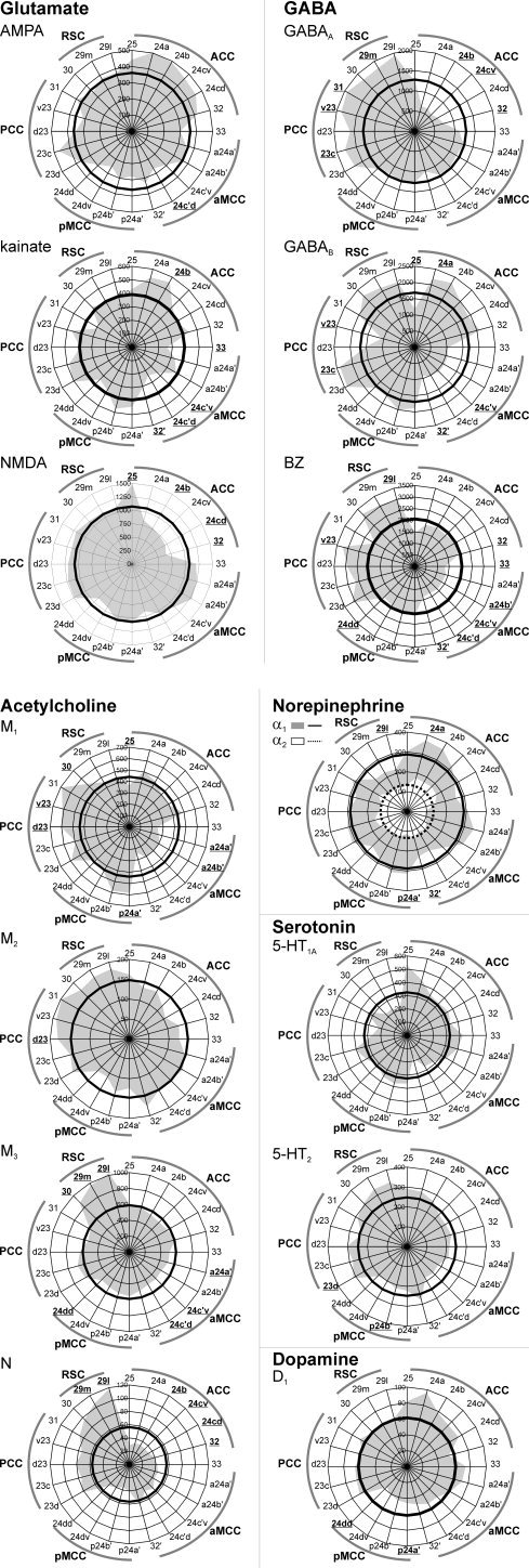
Mean binding site densities (fmol/mg protein; values averaged over all cortical layers) of the 15 receptors displayed as polar coordinate plots. The thick black line in each polar coordinate plot shows the average receptor density of that receptor across all areas. This average value of the α₂ receptor is indicated by a dashed‐black line. Areas containing receptor densities significantly higher or lower than the average density of that across all areas are highlighted for each receptor type in bold and underlined. Highlighted areas in the plot showing α₁ and α₂ receptors indicate significances for the α₁ receptor. In the case of the α₂ receptor only densities of area 24b differed significantly from the average. Although for 5‐HT_1A receptor areal differences from the mean did not reach significance at P < 0.01, they showed a clear tendency to be higher than the average in areas 25 (P = 0.03) and a24a′ (P = 0.03), but lower in areas 24c′d (P = 0.02), v23 (P = 0.02) and 29l (P = 0.02).

AMPA receptors were lower than the average in area 24c′d. Kainate receptors were higher than the average in area 24b, but lower in areas 33, 24c′v, 24c′d, and 32′. NMDA receptors were higher than the average in area 25 and lower in areas 24b, 24cd, and 32.

GABA_A receptor densities were higher than the average in areas 23c, v23, 31, and 29m, but lower in areas 24b, 24cv, and 32. GABA_B receptors were higher than the average in areas 24a and 23c, but lower in areas 25, 24c′v, 32′, and v23. BZ binding site densities were higher than the average in areas v23 and 29l, but lower in areas 32, 33, a24b′, 24c′v, 24c′d, 32′, and 24dd.

M₁ receptor densities were higher than the average in areas p24a′, d23, v23, and 30, but lower in areas 25, a24a′, and a24b′. M₂ receptor densities were higher than the average in area d23. M₃ receptor densities were higher than the average in RSC, but lower in areas a24a′, 24c′v, 24c′d, and 24dd. Nicotinic receptor densities were higher than the average in areas 29m and 29l, but lower in areas 24b, 24cv, 24cd, and 32. The α₁ receptor densities were higher than the average in areas 24a and p24a′, but lower in areas 32′ and 29l. The α₂ receptors were higher than the average in area s24b.

Variations in 5‐HT _1A densities did not reach the level of significance at P < 0.01, although they showed a clear tendency to be higher than the average in areas 25 (P = 0.03) and a24a′ (P = 0.03), but lower in areas 24c′d (P = 0.02), v23 (P = 0.02), and 29l (P = 0.02). 5‐HT₂ receptor densities were higher than the average in area 23d, but lower in area p24b′. D ₁ receptor densities were lower than the average in areas p24a′ and 24dd.

Hierarchical Clustering Analysis

Clustering analysis is typically used to find associations among receptor fingerprints for the full dataset of examined receptors. However, there is no a priori reason to believe that our particular group of 15 receptors will provide the best description among areal plots for the cingulate cortex. Thus, we begin with a hierarchical analysis for all 15 receptors as shown in Figure 5A. It reveals that receptor binding segregates ACC and MCC (Clusters 1–3) from PCC and RSC (Clusters 4 and 5). ACC and MCC contain lower GABA_A, nicotinic and BZ, but higher 5‐HT_1A binding site densities than PCC or RSC. Interestingly, area 25 does not cluster with the remaining areas of ACC (Cluster 1), but is allocated to Cluster 2 and is, therefore, associated with areas of MCC. Receptor binding sites also segregate the anterior (aMCC, Cluster 2) and posterior (pMCC, Cluster 3) components of MCC. The pMCC contains higher GABA_B and BZ but lower AMPA, M₂ and D₁ binding site densities than aMCC. PCC (Cluster 4) and RSC (Cluster 5) differ from each other by the higher M₁ and α₁ but lower M₃ binding site densities in PCC compared with RSC.

Figure 5.

Hierarchical clustering of cingulate regions based on their neurochemical structure. A. Result of the clustering analysis carried out including all receptors and all areas. B. Result of the clustering analysis carried out with all receptors, but excluding RSC areas (29l, 29m, and 30). C. Result of the clustering analysis carried out using all areas but excluding NMDA, GABA_A, GABA_B, and 5‐HT_1A receptors, because their densities in area 25 differ significantly from those of all other ACC areas. D. Result of the clustering analysis carried out using all areas, but only the NMDA, GABA_A, GABA_B, and 5‐HT_1A receptors.

The fact that area 25 does not cosegregate with ACC, but rather with aMCC raises an important question about either the analysis itself, or the hypothesis that area 25 is part of ACC. There are a number of ways to evaluate this question. One strategy is to remove areas from the analysis that have radically different cytoarchitectures and connections, such as those from RSC. This should remove variance from the model and might show tighter associations within areas in the frontal cingulate areas. This approach is shown in Figure 5B and there was no alteration in the position of area 25 in the plot.

Another strategy to evaluate the position of area 25 in the plot is to consider each receptor separately in one of two ways; as a difference of area 25 from the remaining areas located within ACC, or by only using those receptors that are responsible for the segregation itself of area 25. Figuratively, this involves a review of Figure 4 in looking for statistically significant differences between area 25 and all isocortical areas in pACC. This was carried out by means of an ANOVA with repeated measures followed by one‐sample t‐tests as described above. In any instances where all pACC areas differed significantly from the mean area 25 density, the receptor was removed from the analysis. Four receptors achieved significance: NMDA, GABA_A GABA_B, and 5‐HT_1A. Under these conditions, area 25 cosegregated with pACC as predicted by the four‐region neurobiological model (Fig. 5C). Therefore, these four receptors are critical to understanding area 25 in the hierarchical analysis and its association with aMCC.

Finally, a hierarchical analysis incorporating only these four receptors was performed as shown in Figure 5D. With this receptor combination, area 25 cosegregates with aMCC and confirms the pivotal role of these four receptors in the analysis. Area 25 and aMCC contain some of the lowest GABA_B but highest NMDA binding site densities in cingulate cortex. Furthermore, area 25 was characterized by highest 5‐HT_1A receptor densities in cingulate cortex. This relationship raises the question of the laminar distributions of these four receptors in areas 25 and a24′.

DISCUSSION

The aim of this study was an independent evaluation of the human cingulate parcellation scheme and of the four‐region model using a multivariate assessment of binding patterns for 15 neurotransmitter receptors. Statistical analyses of receptor binding revealed that the anterior and posterior portions of Brodmann's area 24 were significantly different. The receptor fingerprints of 15 receptors for classical neurotransmitters distinguished cingulate regions, subregions, and areas. The hierarchical clustering analysis revealed that receptor binding sites segregate ACC, MCC, PCC, and RSC. We were thus able to corroborate the concept of a midcingulate region as an entity which differs structurally and functionally from the anterior cingulate region [Vogt et al.,2003]. Therefore, the four‐region model, including MCC, is based on cytological, connectional, functional, and now receptor fingerprint markers. The cytologically based, receptor confirmed four‐region neurobiological model provides the platform for addressing a wide range of neuronal diseases that impact cingulate cortex.

Cingulate Parcellation Scheme

Receptors for classical neurotransmitters are heterogeneously distributed throughout the human cingulate cortex. Superposition of all borders detected in all examined receptor types by the algorithm‐based quantification of interareal differences in receptor patterns yielded the parcellation scheme of the cingulate cortex based on its receptor architecture.

We demonstrated for the first time the existence of a dorsoventral subdivision of area 24c′ and confirmed the recently described subdivision of area 24c [Palomero‐Gallagher et al.,2008]. Both areas have a portion located on the ventral wall of the cingulate sulcus (24cv and 24c′v) and a portion restricted to the dorsal wall of the cingulate sulcus (24cd and 24c′d). Interestingly, area 24c contains the face part of the rostral cingulate motor area and projects to the facial motor nucleus [Morecraft et al.,1996]. Thus, it is in an excellent position to mediate the expression of facial emotion [Vogt et al.,2003], and its regulation by specific transmitter systems is of particular interest. The presence of a dorsal and a ventral subdivision in human area 24c implies that these two areas (24cv and 24cd) are differentially involved in the facial expression of emotions.

Area 32 of Brodmann has a dysgranular layer IV and a similar area was differentiated into multiple parts based on their adjacent frontal counterparts by von Economo and Koskinas [1925]. Applying cytoarchitectural methods, we were able to show that two parts of area 32 reside in ACC (areas s32 and p32) and one part is found in aMCC (area 32′, [Palomero‐Gallagher et al.,2008; Vogt,1993; Vogt et al.,1995]. Additionally, in our recent study of ACC we demonstrated that areas s32 and p32 differ in their neurochemical structure, as area s32 shows higher AMPA, GABA_B, α₁, 5‐HT_1A, and 5‐HT₂ but lower α₂ receptor concentrations than area p32 [Palomero‐Gallagher et al.,2008]. Here, it is shown that area 32, located dorsal to area 24, and a caudal area 32′, which extends dorsal to area a24′, are not uniform in terms of receptor binding either, and this provides important confirmation of the cytology studies. Area 32 contains considerably higher GABA_B, BZ, M₁, and 5‐HT_1A but lower NMDA and GABA_A binding site densities than area 32′.

Brodmann's area 23 has been divided into dorsal and ventral components using cytological and functional connections [Vogt et al.,2005,2006] and this differentiation was corroborated in this study, because dorsal PCC was found to contain higher GABA_B, M₃ and 5‐HT_1A, but lower M₁ receptor densities than its ventral counterpart. In the monkey, the dPCC receives afferents from the dorsal bank of the principal sulcus, whereas cortex in the rostral tip of both banks projects to vPCC [Vogt and Barbas,1988]. The dPCC, but not vPCC, receives inputs from the central laterocellular, mediodorsal, as well as ventral anterior and ventral lateral thalamic nuclei [Shibata and Yukie,2003; Shima and Tanji,1998]. Additionally, vPCC has reciprocal connections with subgenual ACC [Vogt and Pandya,1987]. Data obtained from imaging studies also suggest a functional segregation of human PCC, with differential involvement of vPCC in spatial representations of personally familiar places and of the dPCC in episodic retrieval of personally familiar places and objects [Sugiura et al.,2005]. Additionally, specification of the dorsal and ventral divisions of PCC as regions of interest in a resting glucose metabolic study showed that they have strikingly different parietal and intracingulate correlations suggesting, among other things, that sensory information flows into these subregions differentially via the dorsal and ventral visual streams [Vogt et al.,2006]. Such differential correlation patterns are further supported by functional connectivity analyses of the components of the brain's “default mode network,” i.e., the cortical regions shown to be active at baseline state in functional magnetic resonance imaging studies [Raichle and Snyder,2007].

Hierarchical Clustering Analysis and the Four‐Region Model

Cingulate areas differ in their mean receptor densities (see Fig. 4) and these variations also occur between different receptor types for a single neurotransmitter, e.g., glutamatergic AMPA and NMDA receptors, or muscarinic M₂ and nicotinic receptors. In accordance with previous reports [Varnäs et al.,2004], area 25 was characterized by highest 5‐HT_1A receptor densities in cingulate cortex. The complex codistribution patterns of various receptors in architectonically defined brain areas indicate the functionally specific balances between the different receptors in each of these different areas [Zilles et al.,2002b]. Furthermore, differences in this site‐specific balance between different receptor types and transmitter systems, i.e., the mean regional densities of several different receptors over all cortical layers in a single, architectonically defined brain region, may represent different hierarchical levels within a functional system.

Analysis of 15 transmitter receptors presents new statistical challenges as well as solutions to assessing the functional organization of cortical regions. In cingulate cortex, for example, receptor binding sites segregate ACC and MCC from PCC and RSC. The ACC and MCC contain lower GABA_A and acetylcholine, but higher AMPA, kainate and 5‐HT_1A binding densities than PCC or RSC. This data is in accordance with results obtained in the monkey cingulate cortex [Bozkurt et al.,2005]. In vivo mapping of cerebral choline acetyltransferase activity [Herholz et al.,2000; Kuhl et al.,1999] revealed comparable distributions of this enzyme in the anterior (areas 24 and 32) and posterior (areas 23 and 31) cingulate cortex, which is in agreement with data obtained in postmortem tissue [Selden et al.,1998]. Choline acetyltransferase is expressed by cholinergic neurons for neurotransmitter synthesis and is the most specific marker of cholinergic activity in the brain. Thus, the gradual increase in muscarinic acetylcholine receptor densities in the rostral‐to‐caudal cingulate areas indicates that ACC, MCC, and PCC are subject to a differential modulation via the cholinergic system.

The hierarchical clustering analysis not only segregates Brodmann's [1909] pre‐ and postcingulate subregions, but clearly shows that the precingulate subregion is not homogeneous, and can be further subdivided into two regions, which we have designated ACC and MCC. This structural subdivision of Brodmann's [1909] precingulate subregion is further supported by numerous functional imaging studies [Botvinick et al.,2004; Davis et al.,2005; Grabenhorst et al.,2007; Holroyd and Coles,2008; Margulies et al.,2007], because no paradigm has ever resulted in an activation of this subregion in its entirety. Rather, activations are restricted to the rostral or caudal portions of the precingulate subregion and are generally designated with the terms “rostral ACC” and “caudal ACC,” respectively. We dispute the use of these denominations because they imply that these are fundamentally the same region and fail to integrate a much wider set of observations. Thus, we do not consider MCC to be a simple caudal subdivision of ACC, because it shows fundamental differences which enable its classification as a qualitatively unique region.

Receptor fingerprints not only support the concept of ACC and MCC regions, but also distinguish among cingulate subregions, such as aMCC from pMCC, further supporting the structural/functional dichotomy within this region [Vogt et al.,2003]. The midcingulate region itself is involved in response selection, whether or not skeletomotor activity is required in a task. As anticipation, mismatch detection, and prediction of behavioral outcomes are relevant to activity in this region, it is involved in premotor planning and has extensive projections to the ventral horn of the spinal cord [Bush, 2008; Dum and Strick,1991; Morecraft and Tanji, 2008]. Part of the rostral premotor area is in sulcal aMCC, while part of the caudal premotor area is in pMCC and both have unique structural features. Also, aMCC has fear‐associated activations, whereas pMCC has no consistent involvement in simple emotions [Phan et al.,2002; Vogt et al.,2003]. In this framework, it is important that the receptor fingerprints distinguish between these subregions and suggest that the level of inhibitory control is critical to this dissociation. Although GABA_A binding is similar in both subregions (see Fig. 4), GABA_B binding is significantly lower in aMCC than in pMCC. This suggests a differential modulation of GABA release in both subregions. The high level of GABA_B binding in pMCC is a feature of lateral motor and premotor areas [Zilles and Palomero‐Gallagher,2001] and we conclude that pMCC shares greater similarities to motor system processing than does aMCC. This expectation is confirmed by the shorter interval between cingulate neuron activity and muscle contraction and limited reward coding in contrast to aMCC [Morecraft and Tanji, 2008].

The Question of Area 25

Interestingly, area 25, a subgenual component of ACC, clustered with areas of aMCC. We determined which of the 15 different receptors are critical to understanding the position of area 25 in the hierarchical analysis and the NMDA, GABA_A GABA_B, and 5‐HT_1A receptors were found to play a pivotal role in its result (Fig. 5D).

The separation of area 25 from the neighboring pACC by its receptor architecture and clustering with aMCC suggests a common circuit organization for parts of cingulate cortex that are anatomically dispersed in the cingulate gyrus. A recent functional imaging study examining the neurocircuitry involved in the processing of valenced information revealed a coactivation of sACC and aMCC, suggesting that they may engage together in particular cingulate functions [Goldstein et al.,2007]. Both area 25 and aMCC are part of a network which is dysfunctional in depression [Johansen‐Berg et al.,2008; Mayberg et al.,2005] and affected by various antidepressant treatments [Goldapple et al.,2004; Mayberg et al.,2005]. Thus, the cosegregation of area 25 with aMCC could be informative in identifying mechanisms of the clinical effects of selective high frequency chronic stimulation of area 25 recently piloted as a novel therapy for treatment resistant depression [Lozano et al.,2008; Mayberg et al.,2005].

It has been known for some time that glucose metabolism in ACC is impaired and serotonin 5‐HT_1A receptor binding is decreased in major depression [Drevets,1999; Drevets et al.,1999]. The selective vulnerability of this transmitter system in cingulate cortex is demonstrated with imaging genetics methods in which the short allele of the 5‐HT transporter is associated with reduced volumes of ACC in prodromal depression [Pezawas et al.,2005]. One of the principal mechanisms of action of the SSRI (selective serotonin receptor uptake inhibitors) antidepressants is via tonic activation of 5‐HT_1A receptors [Haddjeri et al.,1988]. Additionally, polymorphisms in the 5‐HT_1A gene have been associated with response to fluoxetine in major depression [Yu et al.,2006]. Area 25 not only contains the highest 5‐HT_1A receptor densities measured in the cingulate cortex (present results, [Varnäs et al.,2004]), but connectivity studies in the monkey have shown that it also has strong projections to the dorsal raphe [Freedman et al.,2000], which in turn sends serotoninergic projections to most of the cerebral cortex [Conrad et al.,1974; Steinbusch,1984; Vertes,1991]. Thus, area 25 could play an important role in the regulation of serotoninergic neurotransmission [Freedman et al.,2000], and this may be critical to understanding therapeutic responses of depressed patients [Ressler and Mayberg,2007].

In summary, the distribution patterns of receptors for classical neurotransmitters not only demonstrate interareal borders of cingulate areas described by Vogt and coworkers [Vogt and Vogt,2003; Vogt et al.,1995,2001,2003,2004], but enable the further subdivision of areas 24c and 24c′, each of which show a portion located on the ventral wall of the cingulate sulcus (24cv and 24c′v) and a component located on the dorsal wall (24cd and 24c′d) of this sulcus. The site‐specific balance between different receptor types and transmitter systems support the four‐region concept of a structurally and functionally segregated cingulate cortex, though the separation of area 25 from the neighboring pregenual areas of ACC by its receptor architecture and clustering with the aMCC highlights a more complex functional organization of this structure that requires additional investigation. The present strategy suggests new possibilities for analyzing parts of PCC and RSC which are known to have cytological and connection heterogeneities.

REFERENCES

- An X,Bandler R,Öngür D,Price JL ( 1998): Prefrontal cortical projections to longitudinal columns in the midbrain periaqueductal gray in macaque monkeys. J Comp Neurol 401: 544–479. [PubMed] [Google Scholar]
- Botvinick MM,Cohen JD,Carter CS ( 2004): Conflict monitoring and anterior cingulate cortex: An update. Trends Cogn Sci 8: 539–546. [DOI] [PubMed] [Google Scholar]
- Bozkurt A,Zilles K,Schleicher A,Kamper L,Sanz Arigita E,Uylings HB,Kötter R ( 2005): Distributions of transmitter receptors in the macaque cingulate cortex. Neuroimage 25: 219–229. [DOI] [PubMed] [Google Scholar]
- Braak H ( 1976): A primitive gigantopyramidal field buried in the depth of the cingulate sulcus of the human brain. Brain Res 109: 219–233. [DOI] [PubMed] [Google Scholar]
- Broca P ( 1878): Anatomic comparée des circonvolutions cérébrales. Le grand lobe limbique et la scissure limbique dans la série des mammiféres. Rev Anthropol 1: 456–498. [Google Scholar]
- Brodmann K ( 1909): Vergleichende Lokalisationslehre der Großhirnrinde in ihren Prinzipien dargestellt auf Grund des Zellbaues. Leipzig: Barth. [Google Scholar]
- Burgess N ( 2008): Spatial cognition and the brain. Ann N Y Acad Sci 1124: 77–97. [DOI] [PubMed] [Google Scholar]
- Burns SM,Wyss JM ( 1985): The involvement of the anterior cingulate cortex in blood pressure control. Brain Res 340: 71–77. [DOI] [PubMed] [Google Scholar]
- Bush G (in press): Dorsal anterior midcingulate cortex: Roles in normal cognition and disruption in attention deficit/hyperactivity disorder In: Vogt BA,editor. Cingulate Neurobiology & Disease, Vol. 1: Infrastructure, Diagnosis, Treatment. Oxford, UK: Oxford University Press. [Google Scholar]
- Bush G,Vogt BA,Holmes J,Dale AM,Greve D,Jenike MA,Rosen BR ( 2002): Dorsal anterior cingulate cortex: A role in reward‐based decision making. Proc Natl Acad Sci USA 99: 523–528. [DOI] [PMC free article] [PubMed] [Google Scholar]
- Chiba T,Kayahara T,Nakano K ( 2001): Efferent projections of infralimbic and prelimbic areas of the medial prefrontal cortex in the Japanese monkey, Macaca fuscata. Brain Res 888: 83–101. [DOI] [PubMed] [Google Scholar]
- Conrad LC,Leonard CM,Pfaff DW ( 1974): Connections of the median and dorsal raphe nuclei in the rat: An autoradiographic and degeneration study. J Comp Neurol 156: 179–205. [DOI] [PubMed] [Google Scholar]
- Davis KD,Taylor KS,Hutchison WD,Dostrovsky JO,McAndrews MP,Richter EO,Lozano AM ( 2005): Human anterior cingulate cortex neurons encode cognitive and emotional demands. J Neurosci 25: 8402–8406. [DOI] [PMC free article] [PubMed] [Google Scholar]
- Drevets WC ( 1999): Prefrontal cortical‐amygdalar metabolism in major depression. Ann N Y Acad Sci 877: 614–637. [DOI] [PubMed] [Google Scholar]
- Drevets WC,Frank E,Price JC,Kupfer DJ,Holt D,Greer PJ,Huang Y,Gautier C,Mathis C ( 1999): PET imaging of serotonin 1A receptor binding in depression. Biol Psychiatry 46: 1375–1387. [DOI] [PubMed] [Google Scholar]
- Dum RP,Strick PL ( 1991): The origin of corticospinal projections from the premotor areas in the frontal lobe. J Neurosci 11: 667–689. [DOI] [PMC free article] [PubMed] [Google Scholar]
- Dum RP,Strick PL ( 1993): Cingulate motor areas In: Vogt BA,Gabriel M, editors. Neurobiology of Cingulate Cortex and Limbic Thalamus. Boston: Birkhäuser; pp 415–441. [Google Scholar]
- Eickhoff SB,Schleicher A,Scheperjans F,Palomero‐Gallagher N,Zilles K ( 2007): Analysis of neurotransmitter receptor distribution patterns in the cerebral cortex. Neuroimage 34: 1317–1330. [DOI] [PubMed] [Google Scholar]
- Eickhoff SB,Rottschy C,Kujovic M,Palomero‐Gallagher N,Zilles K: Organizational principles of human visual cortex revealed by receptor mapping. Cereb Cortex (in press). [DOI] [PMC free article] [PubMed] [Google Scholar]
- Fernandes KBP,Crippa GE,Tavares RF,Antunes‐Rodrigues J,Corrêa FM ( 2003): Mechanisms involved in the pressor response to noradrenaline injection into the cingulate cortex of unanesthetized rats. Neuropharmacology 44: 757–763. [DOI] [PubMed] [Google Scholar]
- Ferstl EC,von Cramon DY ( 2007): Time, space and emotion: fMRI reveals content‐specific activation during text comprehension. Neurosci Lett 427: 159–164. [DOI] [PubMed] [Google Scholar]
- Freedman LJ,Insel TR,Smith Y ( 2000): Subcortical projections of area 25 (subgenual cortex) of the macaque monkey. J Comp Neurol 421: 172–188. [PubMed] [Google Scholar]
- Geyer S,Ledberg A,Schleicher A,Kinomura S,Schormann T,Bürgel U,Klingberg T,Larsson J,Zilles K,Roland PE ( 1996): Two different areas within the primary motor cortex of man. Nature 382: 805–807. [DOI] [PubMed] [Google Scholar]
- Geyer S,Matelli M,Luppino G,Schleicher A,Jansen Y,Palomero‐Gallagher N,Zilles K ( 1998): Receptor autoradiographic mapping of the mesial motor and premotor cortex of the macaque monkey. J Comp Neurol 397: 231–250. [DOI] [PubMed] [Google Scholar]
- Gittins R,Harrison PJ ( 2004): A quantitative morphometric study of the human anterior cingulate cortex. Brain Res 1013: 212–222. [DOI] [PubMed] [Google Scholar]
- Goldapple K,Segal Z,Garson C,Bieling P,Kennedy S,Mayberg HS ( 2004): Modulation of cortical‐limbic pathways in major depression: treatment specific effects of CBT. Arch Gen Psychiatry 61: 34–41. [DOI] [PubMed] [Google Scholar]
- Goldman‐Rakic PS,Lidow MS,Gallager DW ( 1990): Overlap of dopaminergic, adrenergic, and serotoninergic receptors and complementarity of their subtypes in primate prefrontal cortex. J Neurosci 10: 2125–2138. [DOI] [PMC free article] [PubMed] [Google Scholar]
- Goldstein M,Brendel G,Tuescher O,Pan H,Epstein J,Beutel M,Yang Y,Thomas K,Levy K,Silverman M,Clarkin J,Posner M,Kernberg O,Stern E,Silbersweig D ( 2007): Neural substrates of the interaction of emotional stimulus processing and motor inhibitory control: An emotional linguistic go/no‐go fMRI study. Neuroimage 36: 1026–1040. [DOI] [PubMed] [Google Scholar]
- Grabenhorst F,Rolls ET,Margot C,da Silva MA,Velazco MI ( 2007): How pleasant and unpleasant stimuli combine in different brain regions: odor mixtures. J Neurosci 27: 13532–13540. [DOI] [PMC free article] [PubMed] [Google Scholar]
- Haddjeri N,Blier P,Montigny C ( 1988): Long‐term antidepressant treatments result in a tonic activation of forebrain 5‐HT1A receptors. J Neurosci 18: 10150–10156. [DOI] [PMC free article] [PubMed] [Google Scholar]
- Herholz K,Bauer B,Wienhard K,Kracht L,Mielke R,Lenz MO,Strotmann T,Heiss WD ( 2000): In‐vivo measurements of regional acetylcholine esterase activity in degenerative dementia: Comparison with blood flow and glucose metabolism. J Neural Transm 107: 1457–1468. [DOI] [PubMed] [Google Scholar]
- Holroyd CB,Coles MG ( 2008): Dorsal anterior cingulate cortex integrates reinforcement history to guide voluntary behavior. Cortex 44: 548–559. [DOI] [PubMed] [Google Scholar]
- Iaria G,Chen JK,Guariglia C,Ptito A,Petrides M ( 2007): Retrosplenial and hippocampal brain regions in human navigation: Complementary functional contributions to the formation and use of cognitive maps. Eur J Neurosci 25: 890–899. [DOI] [PubMed] [Google Scholar]
- Johansen‐Berg H,Gutman DA,Behrens TE,Matthews PM,Rushworth MF,Katz E,Lozano AM,Mayberg HS ( 2008): Anatomical connectivity of the subgenual cingulate region targeted with deep brain stimulation for treatment‐resistant depression. Cereb Cortex 18: 1374–1383. [DOI] [PMC free article] [PubMed] [Google Scholar]
- Keene CS,Bucci DJ ( 2008): Involvement of the retrosplenial cortex in processing multiple conditioned stimuli. Behav Neurosci 122: 651–658. [DOI] [PubMed] [Google Scholar]
- Kobayashi Y,Amaral DG ( 2000): Macaque monkey retrosplenial cortex. I. Three‐dimensional and cytoarchitectonic organization. J Comp Neurol 426: 339–365. [DOI] [PubMed] [Google Scholar]
- Kuhl DE,Koeppe RA,Minoshima S,Snyder SE,Ficaro EP,Foster NL,Frey KA,Kilbourn MR ( 1999): In vivo mapping of cerebral acetylcholinesterase activity in aging and Alzheimer's disease. Neurology 52: 691–699. [DOI] [PubMed] [Google Scholar]
- Lidow MS,Goldman‐Rakic PS,Gallager DW,Geschwind DH,Rakic P ( 1989): Distribution of major neurotransmitter receptors in the motor and somatosensory cortex of the rhesus monkey. Neuroscience 32: 609–627. [DOI] [PubMed] [Google Scholar]
- Lozano AM,Mayberg HS,Giacobbe P,Hamani C,Craddock RC,Kennedy SH ( 2008): Subcallosal cingulate gyrus deep brain stimulation for treatment‐resistant depression. Biol Psychiatry 64: 461–467. [DOI] [PubMed] [Google Scholar]
- MacLean PD ( 1990): The Triune Brain in Evolution: Role in Paleocerebral Functions. New York: Plenum Press. [DOI] [PubMed] [Google Scholar]
- Margulies DS,Kelly AM,Uddin LQ,Biswal BB,Castellanos FX,Milham MP ( 2007): Mapping the functional connectivity of anterior cingulate cortex. Neuroimage 37: 579–588. [DOI] [PubMed] [Google Scholar]
- Mayberg HS,Liotti M,Brannan SK,McGinnis S,Mahurin RK,Jerabek PA,Silva JA,Tekell JL,Martin CC,Lancaster JL,Fox PT ( 1999): Reciprocal limbic‐cortical function and negative mood: Converging PET findings in depression and normal sadness. Am J Psychiatry 156: 675–682. [DOI] [PubMed] [Google Scholar]
- Mayberg HS,Lozano AM,Voon V,McNeely HE,Seminowicz D,Hamani C,Schwalb JM,Kennedy SH ( 2005): Deep brain stimulation for treatment‐resistant depression. Neuron 45: 651–660. [DOI] [PubMed] [Google Scholar]
- Merker B ( 1983): Silver staining of cell bodies by means of physical development. J Neurosci Methods 9: 235–241. [DOI] [PubMed] [Google Scholar]
- Meyer G,McElhaney M,Martin W,McGraw CP ( 1973): Stereotactic cingulotomy with results of acute stimulation and serial psychological testing In: Laitinen LV,Livingston KE, editors. Surgical Approaches in Psychiatry. Lancaster: MTP; pp 39–58. [Google Scholar]
- Morecraft RJ,Tanji J (in press): Cingulofrontal interactions and the cingulate motor areas In: Vogt BA,editor. Cingulate Neurobiology & Disease, Vol. 1: Infrastructure, Diagnosis, Treatment. Oxford, UK: Oxford University Press. [Google Scholar]
- Morecraft RJ,Schroeder CM,Keifer J ( 1996): Organisation of face representation in the cingulate cortex of the rhesus monkey. Neuroreport 7: 1343–1348. [DOI] [PubMed] [Google Scholar]
- Morosan P,Rademacher J,Palomero‐Gallagher N,Zilles K ( 2004): Anatomical organization of the human auditory cortex: Cytoarchitecture and transmitter receptors In: Heil P,König E, Budinger E, editors. Auditory Cortex—Towards a Synthesis of Human and Animal Research. Mahwah, New Jersey: Lawrence Erlbaum; pp 27–50. [Google Scholar]
- Neafsey EJ,Terreberry RR,Hurley KM,Ruit KG,Frysztak RJ ( 1993): Anterior cingulate cortex in rodents: Connections, visceral control functions, and implications for emotion In: Kolb B, Tees RC, editors. The Cerebral Cortex of the Rat. Cambridge, MA: MIT; pp 206–223. [Google Scholar]
- O'Hare AJ,Dien J,Waterson LD,Savage CR ( 2008): Activation of the posterior cingulate by semantic priming: A co‐registered ERP/fMRI study. Brain Res 1189: 97–114. [DOI] [PubMed] [Google Scholar]
- Olson CR,Musil SY,Goldberg ME ( 1996): Single neurons in posterior cingulate cortex of behaving macaque: Eye movement signals. J Neurophysiol 76: 3285–3300. [DOI] [PubMed] [Google Scholar]
- Palomero‐Gallagher N,Mohlberg H,Zilles K,Vogt BA ( 2008): Receptor‐ and cytoarchitecture of human anterior cingulate cortex. J Comp Neurol 508: 906–926. [DOI] [PMC free article] [PubMed] [Google Scholar]
- Papez JW ( 1937): A proposed mechanism of emotion. Arch Neurol Psychiatry 38: 725–733. [Google Scholar]
- Parker A,Gaffan D ( 1997): The effect of anterior thalamic and cingulate cortex lesions on object‐in‐place memory in monkeys. Neuropsychologia 35: 1093–1102. [DOI] [PubMed] [Google Scholar]
- Petrides M,Pandya DN ( 2007): Efferent association pathways from the rostral prefrontal cortex in the macaque monkey. J Neurosci 27: 11573–11586. [DOI] [PMC free article] [PubMed] [Google Scholar]
- Pezawas L,Meyer‐Lindenberg A,Drabant EM,Verchinski BA,Munoz KA,Kolachana BS,Egan MF,Mattay VS,Hariri AR,Weinberger DR ( 2005): 5‐HTTLPR polymorphism impacts human cingulate‐amygdala interactions: A genetic susceptibility mechanism for depression. Nat Neurosci 8: 828–834. [DOI] [PubMed] [Google Scholar]
- Phan KL,Wager T,Taylor SF,Liberzon I ( 2002): Functional neuroanatomy of emotion: A meta‐analysis of emotion activation studies in PET and fMRI. Neuroimage 16: 331–348. [DOI] [PubMed] [Google Scholar]
- Pool JL,Ransohoff J ( 1949): Effects on stimulating rostral portion of cingulate gyri in man. J Neurophysiol 12: 385–392. [DOI] [PubMed] [Google Scholar]
- Raichle ME,Snyder AZ ( 2007): A default mode of brain function: A brief history of an evolving idea. Neuroimage 37: 1083–1090. [DOI] [PubMed] [Google Scholar]
- Rakic P,Goldman‐Rakic PS,Gallager DW ( 1988): Quantitative autoradiography of major neurotransmitter receptors in the monkey striate and extrastriate cortex. J Neurosci 8: 3670–3690. [DOI] [PMC free article] [PubMed] [Google Scholar]
- Ressler KJ,Mayberg HS ( 2007): Targeting abnormal neural circuits in mood and anxiety disorders: From the laboratory to the clinic. Nat Neurosci 10: 1116–1124. [DOI] [PMC free article] [PubMed] [Google Scholar]
- Scheperjans F,Grefkes C,Palomero‐Gallagher N,Schleicher A,Zilles K ( 2005a): Subdivisions of human parietal area 5 revealed by quantitative receptor autoradiography: A parietal region between motor, somatosensory and cingulate cortical areas. Neuroimage 25: 975–992. [DOI] [PubMed] [Google Scholar]
- Scheperjans F,Palomero‐Gallagher N,Grefkes C,Schleicher A,Zilles K ( 2005b): Transmitter receptors reveal segregation of cortical areas in the human superior parietal cortex: Relations to visual and somatosensory regions. Neuroimage 28: 362–379. [DOI] [PubMed] [Google Scholar]
- Schleicher A,Amunts K,Geyer S,Kowalski T,Schormann T,Palomero‐Gallagher N,Zilles K ( 2000): A stereological approach to human cortical architecture: Identification and delineation of cortical areas. J Chem Neuroanat 20: 31–47. [DOI] [PubMed] [Google Scholar]
- Selden NR,Gitelman DR,Salamon‐Murayama N,Parrish TB,Mesulam MM ( 1998): Trajectories of cholinergic pathways within the cerebral hemispheres of the human brain. Brain 121: 2249–2257. [DOI] [PubMed] [Google Scholar]
- Shibata H,Yukie M ( 2003): Differential thalamic connections of the posteroventral and dorsal posterior cingulate gyrus in the monkey. Eur J Neurosci 18: 1615–1626. [DOI] [PubMed] [Google Scholar]
- Shima K,Tanji J ( 1998): Role for cingulate motor area cells in voluntary movement selection based on reward. Science 282: 1335–1338. [DOI] [PubMed] [Google Scholar]
- Shima K,Aya K,Mushiake H,Inase M,Aizawa H,Tanji J ( 1991): Two movement‐related foci in the primate cingulate cortex observed in signal‐triggered and self‐paced forelimb movements. J Neurophysiol 65: 188–202. [DOI] [PubMed] [Google Scholar]
- Steinbusch HWM ( 1984): Serotonin‐immunoreactive neurons and their projections in the CNS. Handbook of Chemical Neuroanatomy, Vol. 3: Classical Transmitter and Transmitter receptors in the CNS, Part II. Amsterdam: Elsevier; pp 68–125. [Google Scholar]
- Strick PL,Dum RP,Picard N ( 1998): Motor areas on the medial wall of the hemisphere. Novartis Found Symp 218: 64–75. [DOI] [PubMed] [Google Scholar]
- Sugiura M,Shah NJ,Zilles K,Fink GR ( 2005): Cortical representations of personally familiar objects and places: Functional organization of the human posterior cingulate cortex. J Cogn Neurosci 17: 183–198. [DOI] [PubMed] [Google Scholar]
- Talairach J,Bancaud J,Geier S,Bordas‐Ferrer M,Bonis A,Szikla G ( 1973): The cingulate gyrus and human behavior. Electroencephalogr Clin Neurophysiol 34: 45–52. [DOI] [PubMed] [Google Scholar]
- Varnäs K,Halldin C,Hall H ( 2004): Autoradiographic distribution of serotonin transporters and receptor subtypes in human brain. Hum Brain Mapp 22: 246–260. [DOI] [PMC free article] [PubMed] [Google Scholar]
- Vertes RP ( 1991): A PHA‐L analysis of ascending projections of the dorsal raphe nucleus in the rat. J Comp Neurol 313: 643–668. [DOI] [PubMed] [Google Scholar]
- Vogt BA ( 1993): Structural organization of cingulate cortex: Areas, neurons, and somatodendritic transmitter receptors In: Vogt BA, Gabriel M, editors. Neurobiology of Cingulate Cortex and Limbic Thalamus. A Comprehensive Handbook. Boston: Birkhäuser; pp 19–70. [Google Scholar]
- Vogt BA ( 2005): Pain and emotion interactions in subregions of the cingulate gyrus. Nat Rev Neurosci 6: 533–544. [DOI] [PMC free article] [PubMed] [Google Scholar]
- Vogt BA,Barbas H ( 1988): Structure and connections of the cingulate vocalization region in the rhesus monkey In: Newman JD, editor. The Physiological Control of Mammalian Vocalization. New York: Plenum Press; pp 203–225. [Google Scholar]
- Vogt BA,Laureys S ( 2005): Posterior cingulate, precuneal and retrosplenial cortices: Cytology and components of the neural network correlates of consciousness. Prog Brain Res 150: 205–217. [DOI] [PMC free article] [PubMed] [Google Scholar]
- Vogt BA,Vogt L ( 2003): Cytology of human dorsal midcingulate and supplementary motor cortices. J Chem Neuroanat 26: 301–309. [DOI] [PubMed] [Google Scholar]
- Vogt BA,Pandya DN,Rosene DL ( 1987): Cingulate cortex of the rhesus monkey. I. Cytoarchitecture and Thalamic Afferents. J Comp Neurol 262: 256–270. [DOI] [PubMed] [Google Scholar]
- Vogt BA,Nimchinsky EA,Vogt L,Hof PR ( 1995): Human cingulate cortex: Surface features, flat maps, and cytoarchitecture. J Comp Neurol 359: 490–506. [DOI] [PubMed] [Google Scholar]
- Vogt BA,Vogt L,Perl DP,Hof PR ( 2001): Cytology of human caudomedial cingulate, retrosplenial, and caudal parahippocampal cortices. J Comp Neurol 438: 353–376. [DOI] [PubMed] [Google Scholar]
- Vogt BA,Berger GR,Derbyshire SWG ( 2003): Structural and functional dichotomy of human midcingulate cortex. Eur J Neurosci 18: 3134–3144. [DOI] [PMC free article] [PubMed] [Google Scholar]
- Vogt BA,Hof PR,Vogt LJ ( 2004): Cingulate gyrus In: Paxinos G,Mai JK, editors. The Human Nervous System. Amsterdam: Elsevier; pp 915–949. [Google Scholar]
- Vogt BA,Vogt L,Farber NB,Bush G ( 2005): Architecture and neurocytology of monkey cingulate gyrus. J Comp Neurol 485: 218–239. [DOI] [PMC free article] [PubMed] [Google Scholar]
- Vogt BA,Vogt L,Laureys S ( 2006): Cytology and functionally correlated circuits of human posterior cingulate areas. Neuroimage 29: 452–466. [DOI] [PMC free article] [PubMed] [Google Scholar]
- von Economo C and Koskinas GN ( 1925): Die Cytoarchitektonik der Hirnrinde des erwachsenen Menschen. Wien,Berlin: Springer. [Google Scholar]
- Whalen PJ,Bush G,McNally RJ,Wilhelm S,McInerney SC,Jenike MA,Rauch SL ( 1998): The emotional counting Stroop paradigm: A functional magnetic resonance imaging probe of the anterior cingulate affective division. Biol Psychiatry 44: 1219–1228. [DOI] [PubMed] [Google Scholar]
- Yu YWY,Tsai S‐J,Liou Y‐J,Hong C‐J,Chen T‐J ( 2006): Association study of two serotonin 1A receptor gene polymorphisms and fluoxetine treatment response in Chinese major depressive disorders. Eur Neuropsychopharmacol 16: 498–503. [DOI] [PubMed] [Google Scholar]
- Zilles K,Clarke S ( 1997): Architecture, connectivity, and transmitter receptors of human extrastriate visual cortex. Comparison with nonhuman primates. Cereb Cortex 12: 673–742. [Google Scholar]
- Zilles K,Palomero‐Gallagher N ( 2001): Cyto‐, myelo‐, and receptor architectonics of the human parietal cortex. Neuroimage 14: S8–S20. [DOI] [PubMed] [Google Scholar]
- Zilles K,Palomero‐Gallagher N,Grefkes C,Scheperjans F,Boy C,Amunts K,Schleicher A ( 2002a): Architectonics of the human cerebral cortex and transmitter receptor fingerprints: Reconciling functional neuroanatomy and neurochemistry. Eur Neuropsychopharmacol 12: 587–599. [DOI] [PubMed] [Google Scholar]
- Zilles K,Schleicher A,Palomero‐Gallagher N,Amunts K ( 2002b): Quantitative analysis of cyto‐ and receptorarchitecture of the human brain In: Toga AW,Mazziotta JC, editors. Brain Mapping. The Methods. Amsterdam: Elsevier; pp 573–602. [Google Scholar]
- Zilles K,Palomero‐Gallagher N,Schleicher A ( 2004): Transmitter receptors and functional anatomy of the cerebral cortex. J Anat 205: 417–432. [DOI] [PMC free article] [PubMed] [Google Scholar]