ICA decomposition of EEG signal for fMRI processing in epilepsy

Abstract

In this study, we introduce a new approach to process simultaneous Electroencephalography and functional Magnetic Resonance Imaging (EEG‐fMRI) data in epilepsy. The method is based on the decomposition of the EEG signal using independent component analysis (ICA) and the usage of the relevant components' time courses to define the event related model necessary to find the regions exhibiting fMRI signal changes related to interictal activity. This approach achieves a natural data‐driven differentiation of the role of distinct types of interictal activity with different amplitudes and durations in the epileptogenic process. Agreement between the conventional method and this new approach was obtained in 6 out of 9 patients that had interictal activity inside the scanner. In all cases, the maximum Z‐score was greater in the fMRI studies based on ICA component method and the extent of activation was increased in 5 out of the 6 cases in which overlap was found. Furthermore, the three cases where an agreement was not found were those in which no significant activation was found at all using the conventional approach. Hum Brain Mapp 2009. © 2009 Wiley‐Liss, Inc.

INTRODUCTION

The possibility to record the Electroencephalogram (EEG) inside the Magnetic Resonance (MR) scanner [Ives et al., 1993; Krakow et al., 2000b; Lemieux et al., 1997] has opened the possibility to the study of brain function through simultaneous acquisition of EEG and functional Magnetic Resonance Imaging (fMRI). Although some studies with event related potentials (ERP's) recorded on the EEG have recently appeared in the literature [Debener et al., 2005], showing a relationship between the ERP amplitude and fMRI hemodynamic activation, it is the recording of physiological brain rhythms [Goldman et al., 2002; Laufs et al., 2003a, b] and spontaneous epileptic spiking activity [Hoffmann et al., 2000; Krakow et al., 2000a; Seeck et al., 1998; Warach et al., 1996) that have proved to be the most relevant fields of application so far. Because of its clinical potential in the localization of the sources of interictal epileptiform activity, synchronous EEG‐fMRI is becoming a more common tool in the study of epilepsy.

It is still not clear to what extent localization results from the two approaches (EEG and fMRI) can be expected to be concordant. On a more fundamental approach, Logothetis et al. have reported a good correlation between the fMRI signal and local field potentials within the brain [Logothetis et al., 2001; Logothetis, 2003], which are linked to the EEG potentials observed on the scalp [Niedermeyer and Lopes Da Silva, 1999]. In monkeys, Disbrow et al. [ 2000] have found a spatial overlap of 55% between electrophysiogical measurements on the cortex and fMRI responses in monkeys. Such invasive studies are inherently difficult to conduct in humans, for obvious reasons.

Some initial EEG‐fMRI reports of patients with epilepsy showed a good agreement between fMRI signal increase and EEG source localization [Lemieux et al., 2001]. Others [Bagshaw et al., 2006] noticed that when comparing spatiotemporal dipole modeling with EEG‐fMRI activations and deactivations, on average, the dipoles were 58.5 mm from the voxel with the highest positive t‐value and 32.5 mm from the nearest activated voxel. These values are considerably higher than is generally observed with ERP studies, probably as a result of the relatively widespread field, which can lead to artificially deep dipoles. Better concordance was found when comparing the EEG‐fMRI localizations and stereotaxic EEG (SEEG) [Bénar et al., 2006]. Recently a study comparing concordance between distributed source models and EEG‐fMRI [Grova et al., 2008] showed that good correlation can be found in most patients (6 of 7) but only for few of the clusters (64% of the clusters found in the fMRI showed no correlation).

Nonparametric analysis of the EEG‐fMRI data has been used to prove the robustness of the activation maps obtained by the conventional analysis, by showing that interictal discharges lead to a BOLD response that is significantly different to that obtained by examining random “events” [Waites et al., 2005]. The meaning of the activation maps obtained in EEG‐fMRI studies of epilepsy is still a matter of debate. They are expected to be correlated with the regions of epileptogenesis of interictal activity which might or might not be related to those areas of ictal excitability. Surprisingly, interictal activity can result in either positive or negative activations (in terms of the amplitude of the signal changes) [Aghakhani et al., 2004; Archer et al., 2003). Recent studies observed that deactivations were often found (10/43) in regions associated with the default network, which suggests that those should not be over‐interpreted as clues to regions underlying ictal activity [Kobayashi et al., 2006]. Data obtained with BOLD and arterial spin labelling (ASL) suggests that negative BOLD responses related to interictal epileptic discharges (IED) may arise from the larger blood flow decrease relative to the oxygen consumption decrease, as observed for motor task induced negative BOLD responses in healthy volunteers [Stefanovic et al., 2005]. Bénar et al., [ 2006] have found that the sign of the fMRI response correlates with the low frequency (from 0.5 to 5 Hz) content of the stereotaxic EEG (SEEG) epileptic transients, the latter being a reflection of the slow waves (a higher proportion of energy in the low frequencies of the SEEG was recorded in regions with positive BOLD compared with those of negative BOLD response). This could reflect an increase of metabolism linked to the presence of slow waves (although these are commonly associated with inhibition of neuronal activation). Accordingly, it should be taken into account that increased inhibition can induce positive changes in BOLD response because of enhanced synaptic activity, even if firing rates are overall maintained or even decreased (suffice it to say that if there is a lot of hyperpolarization caused by the activity of inhibitory interneurons, this will cause enhanced neurotransmitter release and synaptic activity with ensuing increased metabolic consumption and a paradoxically lower number of firing pyramidal neurons).

Other studies using EEG‐fMRI data of epileptic patients with IED's have been directed toward investigating the relevance of using different models of the haemodynamic response function (HRF) in the event related design. Although some have proposed patient‐specific HRFs [Kang et al., 2003], others have varied the lag of the HRF [Bagshaw et al., 2004]. The first approach showed an increase in the detectability, but no significant changes in the location of the active regions. The second strategy showed that the canonical response function is sufficiently robust to detect positive BOLD responses, whilst the negative BOLD response seems to be more efficiently detected by using larger lags (up to 9 s).

The utility of temporal clustering analysis (TCA) in the analysis of resting state fMRI of patients with temporal lobe epilepsy [Morgan et al., 2004] has also been shown. Recently [Rodionov et al., 2007) a study showed very good correlation between ICA‐based fMRI (using some prior constraints regarding BOLD‐like spatial and temporal characteristics) and GLM based analysis of EEG‐fMRI of patients with focal epilepsy. The problem with a solely data driven approach is the lack of causality or model behind it.

In this study, Independent Component Analysis (ICA) [Comon, 1994] of the EEG data was evaluated as a potential semiblind (data driven) method to characterize the electric activity of spikes, bursts of spikes and slow waves with different amplitudes and durations. The core mathematical concept of ICA is to minimize the mutual information amongst the data projections. It simply tries to find a coordinate system in which the data projections have minimal temporal overlap.

ICA is already a popular technique to remove artifacts such as eye blinks [Vigário, 1997], eye movement or muscular activity, but because of the high amplitude of interictal activity, and the fact that its sources can be generally considered static, it can also prove important in the separation and identification of such activity [Kobayashi et al., 1999; Urrestarazu et al., 2006]. Ultimately, this method presents a semiautomated approach to detect interictal activity, which might allow reduction of the subjectivity of the evaluation and identification of the epileptiform activity performed by a neurophysiologist.

METHODS

Studies were performed using a 32 channel MRI compatible EEG system (Micromed, Italy), and a 1.5 T MRI scanner (Siemens Symphony, Erlangen, Germany). The EEG acquisition was performed at 2048 Hz. Along with the fMRI data acquisition, structural images were acquired to allow coregistration of the functional maps to the high resolution structural image. The MRI sequence used for acquiring structural images was MPRAGE, 256 × 256 × 104 matrix with a resolution of 0.8 × 0.8 × 1 mm³, whilst the functional studies were carried out using echo planar imaging (EPI) with the following parameters: TE = 40 ms; BW = 1698 Hz/Px; flip angle = 82 degrees; matrix dimensions of 64 × 64 and a spatial resolution of 3 × 3 × 4 mm³. The TR was set to 2.0 s when 24 slices sufficed to perform whole brain coverage (Patients 1‐5 and 7 in Table I) and to 2.5 s when 30 slices were needed (Patients 6, 8, and 9 in Table I). The TE was shorter than in most of fMRI experiments at 1.5 T because the region of interest for most subjects was the temporal lobe. The significant through slice dephasing in such regions reduces the apparent transverse relaxation time, T${}_{\text{2}}^{\text{*}}$. Three runs of 360 volumes each (duration of 12–15 min) were performed inside the scanner for each patient. As a (further) validation procedure, one monitoring EEG study of variable length was performed outside the scanner to evaluate the scalp topography of the interictal activity of each subject in an environment free from cardiobalistogram, gradient and movement artifacts.

Table I.

Overview of the fMRI results obtained with the two processing methods

Patient	Epilepsy type	Number of spikes during EEG‐fMRI	Conventional EEG‐fMRI			EEG‐fMRI based on ICA			General comment	Agreement between Conventional and ICA based EEG‐fMRI
			Position (mm)	Volume (mm3)	Max Z‐score	Position (mm)	Volume (mm3)	Max Z‐score
1	Multiple tubersclerosis complex, two large calcified hamartomas (right frontal lobe, left operculum)	63	(−28,4,4)	3984	4.2	(−22,−25,−53)	44,120	5.04	Positive, located interior to the left hamartoma	yes
						(1,−60,38)	25,880	4.98	Negative	no
2	Multifocal cryptogenic epilepsy without focal lesion	27	(47,24,−5)	2192	4.58	(47,17,−3)	12,784	5.83	positive	yes
3	Frontal lobe epilepsy	127	(−62,−46,9)	5,200	3.43	(−62,−42,7)	8,328	4.23	positive ipsolateral	yes
			(55,−56,19)	5,584	3.52	(55,−60,−19)	8,680	3.93	positive contralateral	yes
4	Cortical dysplasia, right hemisphere parietal and central	20	(23,−79,43)	14,768	5.16	(18,−60,21)	80,304	8.14	Positive, right parietal	yes
			cortical		7.4	cortical	too spread	12.5	negative	yes
5	Cryptogenic focal epilepsy, ictal SPECT shows left frontal lobe hiper‐perfusion	19	(−54,−1,11)	9,528	5.11	(−62,−3,12)	4,856	5.9	positive ipsilateral (left)	yes
			(58,4,12)	10,896	5.21	(60,2,11)	9,120	5.94	positive contralateral (right)	yes
			(4,−69,8)	24,000	4.09	(0,−60,7)	14,560	4.81	positive occipital	yes
6	Parieto‐occipital epilepsy	148				(3,−55,31)	25,088	4.28	Positive	no
7	Right mesial sclerosis	256	(37,0,−13)	14,296	4.98	(36,−1,−17)	16,736	5.27	Positive	yes
						(6,19,−5)	19,712	4.17	positive (ICA1)	no
8	Left mesial sclerosis	14				(−32,−3,−29)	7,376	4.59	positive ipsilateral (right)	no
						(−10,−83,19)	20,728	5.08	positive occipital	no
9	Left mesial sclerosis	105				(30,34,19)	8,488	3.63	positive (right spikes)	no
						(52,−13,34)	7,240	3.52	positive (right spikes)	no

Positions are given in mm in MNI space, and correspond to the center of the activated region. Where columns are left blank, no activation was found. The column “General comment” indicates whether the activation is positively or negatively correlated with the neural activity and whether, if positive, it refers to activity in the region with expected lateralization or elsewhere. Agreement was considered positive when significant overlap between the patches of activation was observed

Fifteen patients who had revealed a very high rate of interictal spike activity in previous monitoring sessions were selected for this study. Out of those fifteen patients, only 10 displayed sufficient interictal activity (five had 1 IED or none and all others had over 6 IED in at least one of the fMRI acquisitions) during our study to allow the fMRI processing to be performed. Out of the 10, one patient had no identifiable interictal activity outside the scanner during the monitoring session that preceded the fMRI study, and as the IED patterns identified during the EEG‐fMRI study had different topographies compared to earlier monitoring sessions, this patient was also excluded. All procedures followed the Declaration of Helsinki, and informed consent was obtained from each patient according to the approved guidelines of the Ethical Committees of the Faculty of Medicine of Coimbra and of the University Hospital of Coimbra.

The EEG data was postprocessed using a Matlab toolbox, EEGLAB (Delorme and Makeig, 2004). The EEG data acquired inside the MRI scanner were corrected for gradient artifacts using the methodology suggested by Allen et al., [ 2000] (using a Gaussian‐weighted mean artifact), followed by the detection of the QRS complex and removal of the cardiobalistogram artifact using algorithms implemented by Niazy [Allen et al., 1998; Niazy et al., 2005). The EEG data was bandpass filtered (1 to 45 Hz), and then down sampled to 128 Hz.

ICA decomposition of the data was performed using the infomax function as implemented on the EEG toolbox [Makeig et al., 1997]. Components with scalp topographies that were consistent both outside and inside the scanner (the ICA decomposition was performed after having concatenated the three EEG‐fMRI runs), and that were also found to be concordant with interictal activity as classified by an epilepsy expert neurophysiologist (only a reduced number of classifications by the neurophysiologist is needed), were selected for further analysis.

To evaluate, by visual inspection, if the component was contaminated with noise because of movement of the subject, the six motion correction parameters (obtained using FLIRT, FSL) were plotted along with the time course of the main components found by the ICA algorithm. Two methods in conjunction were used to reduce noise introduced on the EEG signal by subject head movement: (i) the fMRI and EEG data where movement between consecutive images was larger than 0.5 mm were removed from the analysis and only stretches of data of at least 100 consecutive volumes were kept for further analysis; (ii) ICA components that were consistently present only inside the scanner, and that were found to be closely related to movement artifacts using the method described at the start of the paragraph, were used to decide when the EEG data should be zeroed (because motion artifacts, due to their amplitude and nonlocalized nature, often appear spread through various components of the decomposition).

Two event related models were considered:

• aA model based on spikes and bursts as classified by the neurophysiologist, characterized as a block with a fixed width (100 ms) and amplitude (bursts of spikes were modeled as a succession of independent spikes).
• bA model based on the one or two ICA components that most strongly contribute to explaining the IED activity. The model only considers the signal which is over three standard deviations from the mean of the respective channel, and in those regions, the waveform of the component is kept.

These distinct models of neural activity were then convolved with the canonical HRF to obtain a general linear model (GLM) of the BOLD time course, and the functional data were then processed using FEAT (FMRIB's Software Library, http://www.fmrib.ox.ac.uk/fsl). The following preprocessing steps were applied to the time series of BOLD imaging volumes comprising each dataset: motion correction [Jenkinson et al., 2002]; nonbrain removal [Smith, 2002]; spatial smoothing (using a Gaussian kernel with 6 mm full‐width‐half‐maximum); mean‐based intensity normalization of all volumes by the same factor; and nonlinear high‐pass temporal filtering (using Gaussian‐weighted least squares straight line fitting, with 50 sec cut‐off). A general linear model (GLM) approach with local autocorrelation correction [Woolrich et al., 2001] was used to test for model related activity changes. The first derivatives in respect to time of the models were also included as a regressor, in order to account for any potential variability in the delay of the hemodynamic response across the brain and between subjects. Translation movement parameters and their derivatives were included in the GLM as covariates of no interest. Time‐series statistical analysis was carried out using FILM with local autocorrelation correction [Woolrich et al., 2001]. Z‐ (Gaussian normalized T/F) statistic images were thresholded using clusters determined by Z > 3.0 and a (corrected) cluster significance threshold of P = 0.05 [Worsley et al., 1992]. Higher‐level analysis of the multiple datasets collected from each subject was carried out using a fixed effects model, by forcing the random effects variance to zero in FLAME (FMRIB's Local Analysis of Mixed Effects) [Woolrich et al., 2001].

RESULTS

All the individual results shown hereafter refer to one patient (patient number 7 from Table I), in order to clarify the relevance of all the steps presented in the methodology.

Figure 1 shows the first eight components obtained by applying ICA decomposition to the EEG data outside (Fig. 1a) and inside the MR scanner after preprocessing (Fig. 1b). The patient had been reported to have right medial temporal epilepsy, which is concordant with the components 7 and 3 outside (Fig. 1a) and inside (Fig. 1b) the scanner respectively (note that the order of the components is not necessarily the same). The preprocessed EEG data, acquired both in‐ and outside the scanner, was handed to an experienced neurophysiologist who marked the IED's using the location of maximum amplitude as the time reference. Figure 2 shows the good agreement between the average spike activity measured inside the scanner in the case where all available EEG information is used and in the case when only the main spike‐related component (component 3 shown in Fig. 1b) is projected back in the data.

Figure 1.

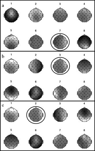
Example of the first eight (out of 32) component scalp maps obtained from ICA decomposition of the EEG data acquired: (a) outside the scanner; (b) inside the scanner (after all gradient and cardiobalistogram artifacts having been removed, and the data having been temporally filtered); (c) inside the scanner after time regions of the EEG data of high activity in components 2 and 4 in the earlier decompositions and movement (as detected by the motion correction) have been set to zero. The black circles highlight the components that were considered to be related to the epileptic spiking activity.

Figure 2.

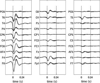
Time courses of the average spike in the different electrodes. The spikes were identified by an expert neurophysiologist. In black, the average EEG data spike is shown whilst in gray only the data resulting from the projection of component 3 (from Fig. 1b) in the data space was used to calculate the average spike activity.

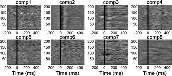
The next step is to evaluate the level of contamination of the main components by the different sources of noise inside the scanner: cardiobalistogram, gradient and movement related artifacts. To evaluate the possible contamination of selected components by cardiac or gradient noise, each component time series was epoched around the corresponding QRS peak as detected by the electrocardiogram (ECG) or scanner trigger. Event related potential (ERP) images were created to control for residual gradient and ballistocardiogram artifacts that might have been isolated in one component. Figure 3 shows the ERP images of the first four components (the topology of these components is shown in Fig. 1b) when considering the cardiac QRS complex peak as a trigger. On the vertical axis, the various cardiac triggers are given whilst the horizontal axis represents time in ms following the cardiac trigger. It can be observed that in components 2 and 4 activity is found which is highly consistent with the cardiac trigger. This is likely to be a residual of the cardiobalistogram artifact which is known to peak at 200 ms. On the other hand, components 1 and 3 (which is the component of interest, as it carries most of the spiking activity related information) don't show such a vertical structure, which means that they do not contain information correlated with the QRS complex. The same analysis can be performed using the volume trigger as an onset for the ERP images to detect components with residual gradient related artifacts. In this specific dataset, no components were found to have significant gradients noise associated with it, and therefore the analysis is not shown. This type of analysis was done in all the subjects and the same conclusion can be taken, no significant gradient or cardiac noise was found on the component attributed to the IEDs.

Figure 3.

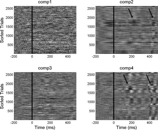
ERP images made using cardiac triggering of the components shown in Figure 1b. ERP images are color‐coded 2D matrices with time on the horizontal axis and different cardiac beats on the vertical axis. Image high intensity corresponds to higher values and low intensities relate to low or negative values. The arrows indicate regions with increased cardiac related artefacts.

In Figure 4 (Bottom half), the temporal derivatives of movement parameters along x and z are plotted against time. This allows a visual comparison with the activity of components 2 and 4, shown above (relating to the ICA decomposition of Fig. 1b) for the same interval. The components are again obtained from the ICA decomposition in Figure 1b. Despite the different sampling rates, it is possible to observe that components 2 and 4 are highly correlated with the movement parameters. As artifacts arising from head movement are highly complex, it is not surprising that those artifacts are not explained by just one or two independent components. In fact, there is often bleeding into a significant number of other components, including those of interest. From our experience, the topologies of components 2 and 4 were found to be highly correlated with movement. For this reason, components with topologies such as 2 and 4 were used to detect movement artifacts: whenever the activity of such components was above a certain threshold, the original EEG data was given the value zero. Finally, a new ICA decomposition was performed, the results of which are shown in Figure 1c.

Figure 4.

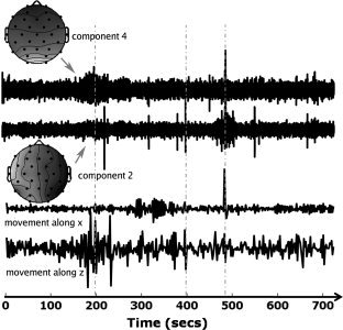
Plots of the activity of components 2 and 4 (relating to the ICA decomposition of Fig. 1b), and of the temporal derivatives of the movement parameters along x and z (bottom) during the same interval (720 seconds). Note that the EEG activity was sampled before the first volume of the EPI was acquired so that any interictal activity preceding the first volume could still be used for general linear model purposes. The units on the y‐axis of the movement plots, and the component time courses are set such that they allow easy visual inspection (each of the curves was normalized so their maximum amplitude is equal to 1). Vertical dashed gray lines represent time points where there is a clear correlation between subject movement and the activity of the selected components.

The choice of the component of interest can be evaluated by looking at the ERP images associated with the spikes marked by the neurophysiologist. Figure 5 shows such an evaluation and it is clear that component 2 (corresponding to the ICA decomposition of Fig. 1c) has the highest correlation with the onset of IEDs identified by the neurophysiologist. It can also be seen that this correlation is not constant throughout the entire dataset, since the last reported spikes, as well as a small region close to the 100th spike, seem to be more correlated with component 3. This suggests that our method, in addition to potentially being able to detect lower amplitude IEDs (which won't necessarily be present on these epochs as they might not have been identified by the neurophysiologist), is also able to discriminate stretches of data where the marking might have been less accurate due to human error or separate IED's with different cortical origin.

Figure 5.

ERP images considering IED marked by a neurophysiologist corresponding to the components with the scalp maps represented in Figure 1c. ERP images are color‐coded 2D matrices with time on the horizontal axis and spikes registered inside the scanner on the vertical axis. This patient had 218 spikes marked. The intensity relates to the components' activations. White corresponds to high values and black relates to negative values.

To rank the level of coherence (vertical structure) of each component, the following expression was used

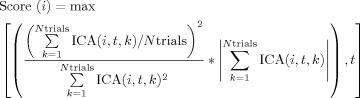(1)

where ICA is now a three‐dimensional matrix where the first two dimensions represent the component number, i, and the epoch time relative to a certain onset, t, and the last dimension represents the IED/volume/QRS number, k, and the notation max[f(i,t),t] means that the maximum is taken along the time dimension. This expression in Eq. (1) evaluates the existence of a vertical structure (across trials) in the ERP image by checking the fraction of power constant across trials (average), 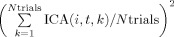, when compared to the overall power, 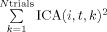for each given time point. However, time intervals or components with good vertical structure but nonsignificant values of activation are not of interest. Thus, the ratio was multiplied by the overall sum of the component's activations for all trials in the time sample of analysis. In this manner, some preference is given to high‐power segments, as it is in these segments that the vertical coherence is of interest. As an example, for the ERP images shown in Figure 5 the following normalized scores were obtained for the first eight components: 0.006; 1.000; 0.046; 0.005; 0.019; 0.006; 0.022; 0.033. Such a quantitative evaluation of the components allows a quick discrimination of the component whose variability is correlated with a certain event (this approach was used also used for detecting components more highly correlated with the cardiobalistogram and scanner artefacts). In this patient's data, it was possible to find that the 11th component had high coherence (Score(11) = 0.21) despite not explaining much of the overall variability.

It should be remarked that the evaluation described above is useful only as a validation of the ability of the ICA to correctly detect interictal activity confirming the overall agreement between the expert detected spikes and the regions of high activity on the component of interest.

The next step is to create the models for the fMRI processing, based on the activity of the component found to best explain the IED (in this case the choice was to use component 2 from Fig. 1c). Because EEG is known to have a typical 1/f noise distribution and one of the first steps in the processing of the EEG data was to apply a band‐pass filter to the data, it seems arbitrary to convolve the component projection information with the HRF. Such an approach would enhance the relevance of low frequency noise in the final model. As the amplitude of the activity is one of the criteria to identify epileptiform activity, in this study an amplitude threshold was used to define the time course regions whose activity was relevant to model the electrical activity of interest. The activity associated with component i is given by ICA(i,t). Because of the arbitrary sign of the components, the neuronal activity was taken to be N(t) = |ICA(i,t)| and made zero when N(t) was lower than n times the temporal standard deviation of the activity of component i. The parameter n was varied in the different analyses between values of 1 and 3, but the results weren't significantly different. All the results shown and discussed refer to n = 3.

In Figure 6, two activation maps obtained from the same dataset are shown based on a conventional (a) and ICA method (b). Although a difference in the extension of the active area obtained with the different methods can be seen, with the ICA method finding more activation in lower slices and apparently losing sensitivity in more superior slices, the majority of the activation maps overlap, (mainly the regions where the activations was found to be most statistically significant). Overall, Figure 6 shows a good agreement between the conventional and ICA method. The increased z‐scores and increased extent of activated regions (see Table I) found when using the interictal related ICA component to model neural activity can also be appreciated in Figure 6. It should be noted that to obtain the results present in Figure 6a using the conventional method, it was necessary to discard the fMRI data corresponding to the IED's over 200 (see Fig. 5) as on a second inspection by the neurophysiologist, these were found to be misclassified and naturally significantly impaired the GLM. Such approach was only used for this dataset, given the clear misidentification of the spiking activity. This fact demonstrates the robustness of the ICA methodology to avoid problems occurring from human error.

Figure 6.

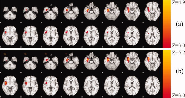
Z‐statistical maps overlaid on structural image from patient 7 obtained (a) using a conventional IED event related approach, and (b) using the proposed method (note that MR images are shown using the radiological convention).

A more detailed overview of the results is given in Table I, which presents a systematic comparison between the results obtained using the conventional method to process EEG‐fMRI and our proposed ICA‐based method.

The main observations that can be drawn from Table I are that: (i) agreement was obtained in 6 of 9 patients; (ii) in all cases the maximum Z‐score was greater in the fMRI studies based on ICA component method and the extent of activation was increased in 5 of the 6 cases in which overlap was found; and (iii) furthermore the three cases where an agreement was not found were those in which no significant activation was found at all using the conventional approach.

Figure 7 shows results from patients 2, 6, 8, and 9 reported in Table I. In Figure 7a,b, it is possible to observe the good agreement between the conventional method and the ICA based method respectively obtained with patient 2. Figures 7b–e show a qualitative congruency between the EEG maps obtained using the ICA (that were found to be highly correlated with spiking activity) and the regions that showed a correlated hemodynamic activity. It should be noted that in patients 6, 8, and 9 (Fig. 7c–e respectively), no significant activation was found using the conventional methodology but a clear congruency between the classification of the epilepsy type based on prior studies (Table I) and regions found active with the proposed methodology was found.

Figure 7.

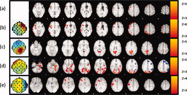
Z‐ statistical maps overlaid on structural image from patient 2 (a,b), 6, 8, and 9 (c–e) using a conventional IED event related approach (a), and using the proposed method (b–e) (note that MR images are shown using the radiological convention).

Negative activations were also found (see Fig. 7d, blue overlay), but their locations were highly uncorrelated with the topologies of the spiking activity and support the hypothesis that spiking activity often occurs in areas associated with the resting state network [Kobayashi et al., 2006].

DISCUSSION

The results of the ICA based method of decomposition of EEG signal for fMRI processing presented here shows very good agreement with the results of a conventional data processing approach when used for EEG‐fMRI analysis and exhibits an increased sensitivity for the detection of brain regions associated with interictal epileptic activity. Several factors contribute to the increased sensitivity of the ICA method described here, particularly the reduced subjectivity in classification of the IED's, which makes it less prone to human error and the fact that lower amplitude activity from the same region might be taken into account. The fact the approach presented in this article is data driven renders it less susceptible to biases introduced by classification or fixed model driven approaches to detect IED's. Often the ability of ICA components to fully characterize an IED is questioned, as in some cases the stationary condition of the sources might not be met, but even in these cases there will be components pinpointing the activity in different regions of the path of the non stationary IED activity, whose activity will be a fair representation of the cortical activity underlying it. ICA decomposition also proved to very reliably separate components that could have information associated with gradient and cardiac noise from the IED activity as was demonstrated in this article.

In a preliminary study, the two methods presented here were compared with a third method resulting from the product of the ICA model and the neurophysiologists marking. In that study, it was observed that Z‐scores obtained using this third approach were comparable (Z _max = 5.5) than to those obtained with the conventional approach (Z _max = 5.7), but lower than those obtained with the proposed method (Z _max = 7.2). Hence, we believe that one of the reasons of the success of this method could be related not only to the significant variability in amplitude and duration of IED's (which the ICA based methods account for in the model used in the fMRI analysis) but also enhanced by the detection of extra activity.

Another attribute of our multimodal method, compared for example to the temporal cluster analysis approaches, is that it benefits from combining analyses of two types of signal and, although data driven on the EEG side, it nevertheless has the advantages associated with a model based analysis of the fMRI data. Therefore the brain regions found to be hemodynamically active can be associated to a certain electrical activity observed in the EEG signal whose topography is known and can be readily recognized or discarded by the neurophysiologist that has followed the patient.

Given the challenges posed during detection of irregular, transient BOLD activity, in particular when the EEG signal quality is degraded because of artefacts caused by motion in the scanner and physiological noise, we believe that our approach proves useful in the context of epilepsy. The technique can be readily extended to other simultaneous EEG‐fMRI studies such as physiological brain rhythms studies [Marques et al., 2006] and cognitive ERP studies coupled with rapid event related fMRI. For the application to the study of brain rhythms, care should be taken in the methodology used for decomposing the EEG signal. The reason why the infomax algorithm is so successful at detecting IED activity is because this algorithm is biased towards supergaussian activity. Rhythmic activity is not necessarily super gaussian (bursts of rhythmic activity are), and therefore, algorithms more biased towards time correlation in the data might prove more powerful [Barros et al., 2000]. Again, the components obtained can be expected to be more uncorrelated with physiological and scanner noise, they are expected to have higher SNR because of being already a combination of the activity in different electrodes, which will improve the quality of the model used for the event related fMRI design.

REFERENCES

- Aghakhani Y,Bagshaw AP,Bénar CG,Hawco C,Andermann F,Dubeau F,Gotman J ( 2004): fMRI activation during spike and wave discharges in idiopathic generalized epilepsy. Brain 127: 1127–1144. [DOI] [PubMed] [Google Scholar]
- Allen PJ,Polizzi G,Krakow K,Fish DR,Lemieux L ( 1998): Identification of EEG events in the MR scanner: The problem of pulse artifact and a method for its subtraction. NeuroImage 8: 229–239. [DOI] [PubMed] [Google Scholar]
- Allen PJ,Josephs O,Turner R ( 2000): A method for removing imaging artifact from continuous EEG recorded during functional MRI. NeuroImage 12: 230–239. [DOI] [PubMed] [Google Scholar]
- Archer JS,Abbott DF,Waites AB,Jackson GD ( 2003): fMRI “deactivation” of the posterior cingulate during generalized spike and wave. Neuroimage 20: 1915–1922. [DOI] [PubMed] [Google Scholar]
- Bagshaw AP,Aghakhani Y,Bénar CG,Kobayashi E,Hawco C,Dubeau F,Pike GB,Gotman J ( 2004): EEG‐fMRI of focal epileptic spikes: Analysis with multiple haemodynamic functions and comparison with gadolinium‐enhanced MR angiograms. Hum Brain Mapp 22: 179–192. [DOI] [PMC free article] [PubMed] [Google Scholar]
- Bagshaw AP,Kobayashi E,Dubeau F,Pike GB,Gotman J ( 2006): Correspondence between EEG‐fMRI and EEG dipole localisation of interictal discharges in focal epilepsy. Neuroimage 30: 417–425. [DOI] [PubMed] [Google Scholar]
- Barros AK,Vigario R,Jousmaki V,Ohnishi N ( 2000): Extraction of event‐related signals from multichannel bioelectrical measurements. IEEE Trans Biomed Eng 47: 583–588. [DOI] [PubMed] [Google Scholar]
- Bénar CG,Grova C,Kobayashi E,Bagshaw AP,Aghakhani Y,Dubeau F,Gotman J ( 2006): EEG‐fMRI of epileptic spikes: Concordance with EEG source localization and intracranial EEG. NeuroImage 30: 1161–1170. [DOI] [PubMed] [Google Scholar]
- Comon P ( 1994): Independent Component Analysis, a New Concept. Signal Process 36: 287–314. [Google Scholar]
- Debener S,Ullsperger M,Siegel M,Fiehler K,von Cramon DY,Engel AK ( 2005): Trial‐by‐trial coupling of concurrent electroencephalogram and functional magnetic resonance imaging identifies the dynamics of performance monitoring. J Neurosci 25: 11730–11737. [DOI] [PMC free article] [PubMed] [Google Scholar]
- Delorme A,Makeig S ( 2004): EEGLAB: an open source toolbox for analysis of single‐trial EEG dynamics. J Neurosci Methods 134: 9–21. [DOI] [PubMed] [Google Scholar]
- Disbrow EA,Slutsky DA,Roberts TP,Krubitzer LA ( 2000): Functional MRI at 1.5 tesla: A comparison of the blood oxygenation level‐dependent signal and electrophysiology. Proc Natl Acad Sci USA 97: 9718–9723. [DOI] [PMC free article] [PubMed] [Google Scholar]
- Goldman RI,Stern JM,Engel J Jr,Cohen MS ( 2002): Simultaneous EEG and fMRI of the alpha rhythm. NeuroReport 13: 2487–2492. [DOI] [PMC free article] [PubMed] [Google Scholar]
- Grova C,Daunizeau J,Kobayashi E,Bagshaw AP,Lina JM,Dubeau F,Gotman J ( 2008): Concordance between distributed EEG source localization and simultaneous EEG‐fMRI studies of epileptic spikes. Neuroimage 39: 755–774. [DOI] [PMC free article] [PubMed] [Google Scholar]
- Hoffmann A,Jager L,Werhahn KJ,Jaschke M,Noachtar S,Reiser M ( 2000): Electroencephalography during functional echo‐planar imaging: Detection of epileptic spikes using post‐processing methods. Magn Reson Med 44: 791–798. [DOI] [PubMed] [Google Scholar]
- Ives JR,Warach S,Schmitt F,Edelman RR,Schomer DL ( 1993): Monitoring the patient's EEG during echo planar MRI. Electroencephalogr Clin Neurophysiol 87: 417–420. [DOI] [PubMed] [Google Scholar]
- Jenkinson M,Bannister P,Brady M,Smith S ( 2002): Improved optimization for the robust and accurate linear registration and motion correction of brain images. NeuroImage 17: 825–841. [DOI] [PubMed] [Google Scholar]
- Kang JK,Bénar CG,Al‐Asmi A,Khani YA,Pike GB,Dubeau F,Gotman J ( 2003): Using patient‐specific hemodynamic response functions in combined EEG‐fMRI studies in epilepsy. NeuroImage 20: 1162–1170. [DOI] [PubMed] [Google Scholar]
- Kobayashi K,James CJ,Nakahori T,Akiyama T,Gotman J ( 1999): Isolation of epileptiform discharges from unaveraged EEG by independent component analysis. Clin Neurophysiol 110: 1755–1763. [DOI] [PubMed] [Google Scholar]
- Kobayashi E,Bagshaw AP,Grova C,Dubeau F,Gotman J ( 2006): Negative BOLD responses to epileptic spikes. Hum Brain Mapp 27: 488–497. [DOI] [PMC free article] [PubMed] [Google Scholar]
- Krakow K,Allen PJ,Lemieux L,Symms MR,Fish DR ( 2000a): Methodology: EEG‐correlated fMRI. Adv Neurol 83: 87–201. [PubMed] [Google Scholar]
- Krakow K,Allen PJ,Symms MR,Lemieux L,Josephs O,Fish DR ( 2000b): EEG recording during fMRI experiments: Image quality. Hum Brain Mapp 10: 10–15. [DOI] [PMC free article] [PubMed] [Google Scholar]
- Laufs H,Kleinschmidt A,Beyerle A,Eger E,Salek‐Haddadi A,Preibisch C,Krakow K ( 2003a): EEG‐correlated fMRI of human α activity. NeuroImage 19: 1463–1476. [DOI] [PubMed] [Google Scholar]
- Laufs H,Krakow K,Sterzer P,Eger E,Beyerle A,Salek‐Haddadi A,Kleinschmidt A ( 2003b): Electroencephalographic signatures of attentional and cognitive default modes in spontaneous brain activity fluctuations at rest. Proc Natl Acad Sci USA 100: 11053–11058. [DOI] [PMC free article] [PubMed] [Google Scholar]
- Lemieux L,Allen PJ,Franconi F,Symms MR,Fish DR ( 1997): Recording of EEG during fMRI experiments: Patient safety. Magn Reson Med 38: 943–952. [DOI] [PubMed] [Google Scholar]
- Lemieux L,Salek‐Haddadi A,Josephs O,Allen P,Toms N,Scott C,Krakow K,Turner R,Fish DR ( 2001): Event‐related fMRI with simultaneous and continuous EEG: Description of the method and initial case report. NeuroImage 14: 780–787. [DOI] [PubMed] [Google Scholar]
- Logothetis NK ( 2003): The underpinnings of the BOLD functional magnetic resonance imaging signal. J Neurosci 23: 3963–3971. [DOI] [PMC free article] [PubMed] [Google Scholar]
- Logothetis NK,Pauls J,Augath M,Trinath T,Oeltermann A ( 2001): Neurophysiological investigation of the basis of the fMRI signal. Nature 412: 150–157. [DOI] [PubMed] [Google Scholar]
- Makeig S,Jung TP,Bell AJ,Ghahremani D,Sejnowski TJ ( 1997): Blind separation of auditory event‐related brain responses into independent components. Proc Natl Acad Sci USA 94: 10979–10984. [DOI] [PMC free article] [PubMed] [Google Scholar]
- Marques JP,Figueiredo P,Sales F,Castelo‐Branco M ( 2006): On the usage of ICA decomposition of EEG signal for fMRI processing. In: 12th Annual Meeting of the Organization for Human Brain Mapping, Florence, Italy. p S72. [DOI] [PMC free article] [PubMed]
- Morgan VL,Price RR,Arain A,Modur P,Abou‐Khalil B ( 2004): Resting functional MRI with temporal clustering analysis for localization of epileptic activity without EEG. NeuroImage 21: 473–481. [DOI] [PubMed] [Google Scholar]
- Niazy RK,Beckmann CF,Iannetti GD,Brady JM,Smith SM ( 2005): Removal of FMRI environment artifacts from EEG data using optimal basis sets. NeuroImage 28: 720–737. [DOI] [PubMed] [Google Scholar]
- Niedermeyer E,Lopes Da Silva FH ( 1999): Electroencephalography: Basic principles, Clinical Applications and Related Fields, 4th ed United States: Lippincott Williams and Wilkins. [Google Scholar]
- Rodionov R,De Martino F,Laufs H,Carmichael DW,Formisano E,Walker M,Duncan JS,Lemieux L ( 2007): Independent component analysis of interictal fMRI in focal epilepsy: Comparison with general linear model‐based EEG‐correlated fMRI. NeuroImage 38: 488–500. [DOI] [PubMed] [Google Scholar]
- Seeck M,Lazeyras F,Michel CM,Blanke O,Gericke CA,Ives J,Delavelle J,Golay X,Haenggeli CA,de Tribolet N,Landis T ( 1998): Non‐invasive epileptic focus localization using EEG‐triggered functional MRI and electromagnetic tomography. Electroencephalogr Clin Neurophysiol 106: 508–512. [DOI] [PubMed] [Google Scholar]
- Smith SM ( 2002): Fast robust automated brain extraction. Hum Brain Mapp 17: 143–155. [DOI] [PMC free article] [PubMed] [Google Scholar]
- Stefanovic B,Warnking JM,Kobayashi E,Bagshaw AP,Hawco C,Dubeau F,Gotman J,Pike GB ( 2005): Hemodynamic and metabolic responses to activation, deactivation and epileptic discharges. NeuroImage 28: 205–215. [DOI] [PubMed] [Google Scholar]
- Urrestarazu E,Iriarte J,Artieda J,Alegre M,Valencia M,Viteri C ( 2006): Independent component analysis separates spikes of different origin in the EEG. J Clin Neurophysiol 23: 72–78. [DOI] [PubMed] [Google Scholar]
- Vigário RN ( 1997): Extraction of ocular artefacts from EEG using independent component analysis. Electroencephalogr Clin Neurophysiol 103: 395–404. [DOI] [PubMed] [Google Scholar]
- Waites AB,Shaw ME,Briellmann RS,Labate A,Abbott DF,Jackson GD ( 2005): How reliable are fMRI‐EEG studies of epilepsy? A nonparametric approach to analysis validation and optimization. Neuroimage 24: 192–199. [DOI] [PubMed] [Google Scholar]
- Warach S,Ives JR,Schlaug G,Patel MR,Darby DG,Thangaraj V,Edelman RR,Schomer DL ( 1996): EEG‐triggered echo‐planar functional MRI in epilepsy. Neurology 47: 89–93. [DOI] [PubMed] [Google Scholar]
- Woolrich MW,Ripley BD,Brady M,Smith SM ( 2001): Temporal autocorrelation in univariate linear modeling of FMRI data. NeuroImage 14: 1370–1386. [DOI] [PubMed] [Google Scholar]
- Worsley KJ,Evans AC,Marrett S,Neelin P ( 1992): A three‐dimensional statistical analysis for CBF activation studies in human brain. J Cereb Blood Flow Metab 12: 900–918. [DOI] [PubMed] [Google Scholar]