

Abstract
Voxel‐based analysis (VBA) methods are increasingly being used to compare diffusion tensor image (DTI) properties across different populations of subjects. Although VBA has many advantages, its results are highly dependent on several parameter settings, such as those from the coregistration technique applied to align the data, the smoothing kernel, the statistics, and the post‐hoc analyses. In particular, to increase the signal‐to‐noise ratio and to mitigate the adverse effect of residual image misalignments, DTI data are often smoothed before VBA with an isotropic Gaussian kernel with a full width half maximum up to 16 × 16 × 16 mm3. However, using isotropic smoothing kernels can significantly partial volume or voxel averaging artifacts, adversely affecting the true diffusion properties of the underlying fiber tissue. In this work, we compared VBA results between the isotropic and an anisotropic Gaussian filtering method using a simulated framework. Our results clearly demonstrate an increased sensitivity and specificity of detecting a predefined simulated pathology when the anisotropic smoothing kernel was used. Hum Brain Mapp, 2010. © 2009 Wiley‐Liss, Inc.
Keywords: diffusion tensor imaging, voxel‐based analysis, smoothing
INTRODUCTION
Diffusion tensor magnetic resonance imaging (DT‐MRI or DTI) is a unique, noninvasive imaging technique that provides an insight into the complex brain white matter (WM) connectivity [Basser et al.,1994]. As a microstructural breakdown of WM is present in a wide range of diseases, quantitative DTI measures have a tremendous potential to assess tissue damage in these pathologies. To reveal subtle, microstructural WM changes in different pathologies, standardized and reliable postprocessing algorithms are needed. A widely used automated approach to analyze a group of DTI data sets is provided by a voxel‐based analysis (VBA). In a VBA setting, all data sets are generally transformed to an atlas, whereafter a voxel‐by‐voxel statistical comparison of diffusion measures between control subjects and patients is performed [Ashburner and Friston,2000]. Before applying the statistical analysis, the data sets are smoothed with an isotropic Gaussian kernel to increase the signal‐to‐noise ratio (SNR) and to mitigate the adverse effect of residual image misalignments. In this context, the matched filter theorem states that a signal is detected with an optimal sensitivity if a convolution kernel is used that matches the size and shape of the signal change [Rosenfeld and Kak,1982]. Based on this matched filter theorem, a “rule of thumb” is often used in the analysis of fMRI and PET data sets. This rule of thumb states that the full width at half maximum (FWHM) of the smoothing kernel should at least be two to three times the voxel dimension when analyzing data of a single subject, and even larger for a group analysis, because this FWHM corresponds to the hemodynamic response that should be detected [Friston et al.,1996; Petersson et al.,1999; Worsley et al.,1992].
According to the matched filter theorem, the sensitivity of the pathology detection in a DTI group study will be improved when the data sets are smoothed with a kernel size that exactly matches the extent of the expected pathology [Rosenfeld and Kak,1982]. As this extent is rarely known a priori, it is very hard to determine the optimal Gaussian kernel width to smooth the DTI data sets. Consequently, in the DTI‐VBA literature, a large range of uniform, isotropic smoothing kernel widths up to as much as 16 mm is used (see Table I for an overview and references). This large variability of the smoothing kernel width across studies is particularly problematic because Foong et al. [2002], Park et al. [2004], and Jones et al. [2005] demonstrated that the reported VBA results depend on the applied smoothing kernel width. The matched filter theorem also states that, apart from the size, the shape of the smoothing kernel should correspond to the expected signal differences. Although the shape of pathology is rarely known in advance, it will most likely follow the affected WM fiber bundle, without harming nearby cerebrospinal fluid (CSF) or gray matter (GM) tissue. To the best of our knowledge, all published VBA studies based on DT images use a uniform, isotropic Gaussian smoothing kernel, which increases the risk of averaging signal intensities across anatomically distinct structures before the application of the voxel‐wise statistical testing (see Table I).
Table I.
An overview of the full width at half maximum (FWHM) of the isotropic smoothing kernels that have been used in published VBA studies of DTI data sets
| Reference | Voxel size(mm3) | FWHM(mm3) | FWHM(voxels) | Number of subjects |
|---|---|---|---|---|
| Ardekani et al.,2003 | 1.8 × 1.8 × 5 | 0 × 0 × 0 | 0 × 0 × 0 | 28 |
| Park et al.,2004 | 1.7 × 1.3 × 4 | 3 × 3 × 3 | 1.8 × 2.3 × 0.8 | 55 |
| Barnea‐Goraly et al.,2003 | 1.9 × 1.9 × 5 | 4 × 4 × 4 | 2.1 × 21 × 0.8 | 20 |
| Barnea‐Goraly et al.,2004 | 1.9 × 1.9 × 5 | 4 × 4 × 4 | 2.1 × 21 × 0.8 | 25 |
| Barnea‐Goraly et al.,2005 | 1.9 × 1.9 × 5 | 4 × 4 × 4 | 2.1 × 21 × 0.8 | 34 |
| Holzapfel et al.,2006 | 1.9 × 1.9 × 5 | 4 × 4 × 4 | 2.1 × 21 × 0.8 | 20 |
| Kyriakopoulos et al.,2007 | 1.9 × 1.9 × 2.5 | 4 × 4 × 4 | 2.1 × 21 × 1.6 | 39 |
| Shergill et al.,2007 | 2.5 × 2.5 × 2.5 | 4 × 4 × 4 | 1.6 × 1.6 × 1.6 | 79 |
| Snook et al.,2007 | 2.3 × 1.7 × 3 | 4 × 4 × 4 | 1.7 × 2.4 × 1.3 | 60 |
| Vangberg et al.,2006 | 1.8 × 1.8 × 5 | 4 × 4 × 4 | 2.2 × 2.2 × 0.8 | 123 |
| Golestani et al.,2006 | 0.94 × 0.94 × 2 | 5 × 5 × 5 | 5.3 × 5.3 × 2.5 | 33 |
| Ng et al.,2008 | 2.2 × 2.2 × 5 | 5 × 5 × 5 | 2.3 × 2.3 × 1 | 21 |
| Molko et al.,2004 | 1.9 × 1.9 × 2.8 | 5 × 5 × 5 | 2.6 × 2.6 × 1.8 | 28 |
| Nagy et al.,2003 | 1.7 × 1.7 × 5 | 5 × 5 × 5 | 2.9 × 2.9 × 1 | 19 |
| Rose et al.,2008 | 1.9 × 1.9 × 5 | 5 × 5 × 5 | 2.6 × 2.6 × 1 | 26 |
| White et al.,2007 | 2 × 2 × 2 | 5 × 5 × 5 | 2.5 × 2.5 × 2.5 | 30 |
| Foong et al.,2002 | 2.5 × 2.5 × 5 | 6 × 6 × 6 | 2.4 × 2.4 × 1.2 | 33 |
| Li et al.,2007 | 1.9 × 1.9 × 3 | 6 × 6 × 6 | 3.2 × 3.2 × 2 | 17 |
| Park et al.,2004 | 1.7 × 1.3 × 4 | 6 × 6 × 6 | 3.6 × 4.6 × 1.6 | 55 |
| Sach et al.,2004 | 3 × 3 × 3 | 6 × 6 × 6 | 2 × 2 × 2 | 27 |
| Sage et al.,2007 | 2 × 2 × 2.2 | 6 × 6 × 6 | 3 × 3 × 2.7 | 60 |
| Seok et al.,2007 | 1.7 × 1.7 × 2 | 6 × 6 × 6 | 3.5 × 3.5 × 3 | 52 |
| Chappell et al.,2006 | 1.7 × 1.7 × 5 | 8 × 8 × 8 | 4.7 × 4.7 × 1.6 | 93 |
| Erikkson et al.,2001 | 2.5 × 2.5 × 5 | 8 × 8 × 8 | 3.2 × 3.2 × 1.6 | 52 |
| Focke et al.,2008 | 1.9 × 1.8 × 2.4 | 8 × 8 × 8 | 4.2 × 4.4 × 3.3 | 58 |
| Gimenez et al.,2008 | 1.8 × 1.8 × 3.4 | 8 × 8 × 8 | 4.4 × 4.4 × 2.4 | 37 |
| Menzies et al.,2008 | 2.3 × 1.9 × 4 | 8 × 8 × 8 | 3.5 × 4.2 × 2 | 60 |
| Pagani et al.,2008 | 1.9 × 1.9 × 4 | 8 × 8 × 8 | 4.2 × 4.2 × 2 | 84 |
| Park et al.,2004 | 1.7 × 1.3 × 4 | 9 × 9 × 9 | 4.8 × 6.9 × 2.4 | 55 |
| Porto et al.,2008 | 2 × 2 × 2 | 9 × 9 × 9 | 4.5 × 4.5 × 4.5 | 21 |
| Albrecht et al.,2007 | 1.8 × 1.8 × 4 | 10 × 10 × 10 | 5.6 × 5.6 × 3.3 | 45 |
| Borroni et al.,2007 | 1.7 × 1.7 × 5 | 10 × 10 × 10 | 5.9 × 5.9 × 2 | 59 |
| Borroni et al.,2008 | 1.7 × 1.7 × 5 | 10 × 10 × 10 | 5.9 × 5.9 × 2 | 31 |
| Erikkson et al.,2001 | 2.5 × 2.5 × 5 | 10 × 10 × 10 | 4 × 4 × 2 | 52 |
| Kumar et al.,2006 | 1.8 × 1.8 × 2 | 10 × 10 × 10 | 5.6 × 5.6 × 5 | 30 |
| Shin et al.,2006 | 1.7 × 1.7 × 4 | 10 × 10 × 10 | 5.9 × 5.9 × 2.5 | 40 |
| Skelly et al.,2008 | 1.6 × 2 × 3 | 10 × 10 × 10 | 6.3 × 5 × 3.3 | 50 |
| Thivard et al.,2007 | 1.3 × 1.3 × 5 | 10 × 10 × 10 | 7.7 × 7.7 × 2 | 40 |
| Padovani et al.,2005 | 1.7 × 1.7 × 5 | 10 × 10 × 10 | 5.9 × 5.9 × 2 | 28 |
| Burns et al.,2003 | 1.9 × 1.9 × 5 | 12 × 12 × 12 | 6.4 × 6.4 × 2.4 | 60 |
| Ceccarelli et al.,2008 | 2.5 × 2.5 × 2.5 | 12 × 12 × 12 | 4.8 × 4.8 × 4.8 | 40 |
| Bruno et al.,2008 | 2.5 × 2.5 × 5 | 15 × 15 × 15 | 6 × 6 × 3 | 64 |
| Foong et al.,2002 | 2.5 × 2.5 × 5 | 16 × 16 × 16 | 6.4 × 6.4 × 3.2 | 33 |
| Mean | 1.9 × 1.9 × 3.9 | 7.6 × 7.6 × 7.6 | 3.9 × 4 × 2.2 | 44 |
| SD | 0.4 × 0.4 × 1.2 | 3.2 × 3.2 × 3.2 | 1.7 × 1.7 × 1 | 22 |
The voxel size of the acquired images and the FWHM of the applied smoothing kernel (in mm) are displayed in the second and third column, respectively, In the fourth column, the FWHM of the smoothing in units of the corresponding voxel size is presented. In addition, the total number of subjects that were used in these studies is displayed in the right column.
Perona and Malik [1990] developed an anisotropic diffusion scheme for image data, where the diffusion and flow functions are guided by local gradient strengths in different directions. In this way, noise is removed in homogeneous regions, whereas object boundaries are preserved and edges are sharpened. Anisotropic smoothing has already been applied to denoise DTI data sets [Chen and Hsu,2005; Ding et al.,2005; Fillard et al.,2007; Martin‐Fernandez et al.,2009]. In these studies, using real and synthetic data, it has been demonstrated that the underlying information is better preserved after anisotropic compared with isotropic filtering. Recently, a tissue‐specific, smoothing‐compensated method was proposed by Lee et al. [2009].
In this work, the effect of different isotropic and anisotropic smoothing kernel widths are evaluated in a VBA setting for DT images. To this end, an adaptive anisotropic diffusion filter was applied to the FA maps [Sijbers et al.,1999]. Simulated DTI data sets with a predefined pathology (i.e., a known size, shape, location, and level of FA decrease) were hereby used to compare the VBA sensitivity and specificity after isotropic as well as anisotropic smoothing. Our results clearly demonstrate an increased sensitivity and specificity of detecting this predefined simulated pathology when the anisotropic smoothing kernel was applied.
METHODS
Constructing Simulated DTI Data Sets
Recently, we developed a framework to construct realistic, simulated DTI data sets that contain a predefined pathology [Van Hecke et al.,2009]. This simulation framework for DT images is presented schematically in Figure 1 and can be summarized as follows [Van Hecke et al.,2009]:
After correcting the diffusion‐weighted images for motion and distortion artifacts, the diffusion tensor is estimated nonlinearly while taking the rotation of the b‐matrix into account [Leemans and Jones,2009] (Fig. 1A).
From the EPI Montreal Neurological Institute (MNI) template, a custom FA‐based template was constructed as described in Jones et al. [2002]. All DTI data sets were transformed to this FA atlas with an affine transformation using MIRIT (Multimodality Image Registration using Information Theory) based on the FA maps (Fig. 1B) [Maes et al.,1997]. The preservation of principal direction (PPD) tensor reorientation strategy was thereby incorporated [Alexander et al.,2001; Leemans et al.,2005].
From the affinely aligned data sets, a population specific DTI atlas was constructed by transforming the data sets nonrigidly to the population specific atlas space using a viscous fluid model and mutual information (Fig. 1C,D) [Van Hecke et al.,2007,2008].
The resulting atlas was regarded as the fundamental image and was copied N times (Fig. 1E). In half of these N atlases, the diffusion properties were altered in known WM locations to simulate different pathologies (Fig. 1F). In this study, the transverse diffusivity, that is, the average of the second and third eigenvalues, was increased by six different levels to simulate a microstructural breakdown in 19 WM structures (see Fig. 2). These six levels of pathology correspond with an average FA decrease of 7, 10, 13, 16, 19, and 22%. Similar FA decreases were reported in DTI data sets of diseased subjects in the literature, such as for example in the study of multiple sclerosis [Audoin et al.,2007; Cercignani et al.,2002; Ge et al.,2004; Hasan et al.,2005; Oh et al.,2004; Yu et al.,2007].
Intersubject variability of the diffusion properties was introduced in all atlas images (Fig. 1G). Simulation of the intersubject variance was obtained using a principal component analysis (PCA) on the longitudinal and the transverse eigenvalue images, because they contain all the information regarding the local diffusion properties. Based on the eigenvalue images of 60 healthy subjects, the eigenvalue variability was calculated and samples were added to the simulated DTI data sets [Van Hecke et al.,2009]. Thereafter, the DW images were back‐reconstructed from the DT data.
Rician noise was added to the DW images (Fig. 1H) to obtain simulated data sets with a realistic noise level. As a result, simulated DTI data sets with a SNR of 18 were obtained, which is similar to the noise level of real DT images [Van Hecke et al.,2009].
Figure 1.
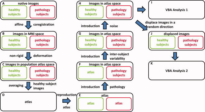
In the construction framework of the simulated data sets, native images of healthy and pathology subjects (A) are transformed to the MNI template using an affine transformation (B). Thereafter, a DTI atlas is constructed from these images (C, D). This atlas is reproduced N times (E) and a simulated pathology is added in half of these atlas data sets (F). Subsequently, intersubject variability (G) and noise (H) are added to all images. The resulting data sets are used in the VBA Analysis 1 (I). In VBA Analysis 2, these data sets are first displaced in a random direction by different distances (J, K). [Color figure can be viewed in the online issue, which is available at www.interscience.wiley.com.]
Figure 2.
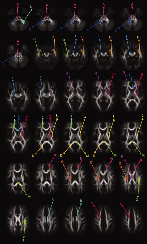
The simulated pathology is visualized on 30 axial FA slices. Here, the various pathology clusters are each given a different color: A: Corticospinal tract; B, C: cerebellar peduncle; D, E: inferior longitudinal fasciculus; F: cerebral peduncle; G: anterior limb of the capsula interna; H: posterior limb of the internal capsule; I: genu of the corpus callosum; J: forceps minor; K: forceps major; L: capsula externa; M: splenium of the corpus callosum; N: anterior region of the corona radiata; O: superior region of the corona radiata; P: body of the corpus callosum; Q: superior longitudinal fasciculus; R: cingulum; and S: superior region of the corona radiata. [Color figure can be viewed in the online issue, which is available at www.interscience.wiley.com.]
Image Acquisition
DTI data sets were obtained on a 1.5 T MR scanner using an SE‐EPI sequence with the following acquisition parameters: TR: 10.4 s; TE: 100 ms; diffusion gradient: 40 mT m−1; FOV = 256 × 256 mm2; number of slices = 60; voxel size = 2 × 2 × 2 mm3; b‐value of 700 s mm−2; and acquisition time: 12 min 18 s. Diffusion measurements were performed along 60 directions with 10 b0‐images for a robust estimation of the diffusion tensors [Jones,2004]. All DTI data sets were processed with “ExploreDTI” [Leemans et al.,2009].
In correspondence with the average number of DTI data sets that is used in the VBA literature, 20 (=N/2) simulated healthy subject and 20 simulated pathology subject DTI data sets are constructed (see Table I). In total, 100 DTI data sets were acquired. Twenty DTI data sets were obtained from pathology subjects with multiple sclerosis. These data sets, together with 20 healthy subject data sets that were age‐ and sex‐matched with the MS patient images, were used to make the database. The remaining 60 healthy subject data sets were used to construct the intersubject variability maps.
To study the effect of the pathology size on the VBA results for different smoothing kernels, the group of pathologies is divided in three subgroups: small (i.e., number of voxels smaller than 50), medium (i.e., number of voxels between 50 and 65), and large (i.e., number of voxels larger than 65) pathologies. These thresholds were chosen so that an equal number of pathologies is present in each subgroup.
Smoothing Methods
Anisotropic smoothing methods have already been applied to reduce the noise contribution in DTI data sets [Chen and Hsu,2005; Ding et al.,2005; Fillard et al.,2007; Martin‐Fernandez et al.,2009]. However, to the best of our knowledge, these advanced filtering approaches have not been used before in a DTI‐based VBA setting. In all VBA studies of DT images, a uniform, isotropic, Gaussian smoothing kernel was used before applying the statistical tests (see Table I for an overview with references).
In the following sections, both the isotropic and the anisotropic Gaussian smoothing approach are described
Uniform, isotropic smoothing
Consider an image
 with
with
 a three‐dimensional position vector. A filtering algorithm computes a new image
 by applying at each point
 a kernel
 to the original image
 , within a neighborhood Ω:
| (1) |
When the kernel is invariant over space, that is, when
 does not depend on
 , the image is uniformly smoothed. In the case of isotropic Gaussian smoothing,
 can be written as:
| (2) |
To evaluate the effect of the isotropic smoothing kernel size σ on the sensitivity and the specificity of the VBA results, the FA maps of the simulated data sets are smoothed with kernels that have Gaussian standard deviations σ of 1.27, 2.54, 3.81, and 5.08 mm, corresponding with a FWHM of 3, 6, 9, and 12 mm, respectively.
Anisotropic smoothing
In this work, the method of Sijbers et al. [1999] was used to smooth the FA maps anisotropically before applying the voxel‐wise statistical tests. The basic idea behind the anisotropic adaptive noise filter is that
 of Eq. (1) is made variable and allowed to be shaped or scaled according to local image features within the neighborhood Ω of
 . This results in the following anisotropic adaptive Gaussian filter:
| (3) |
with
 corresponding to the main axes of the local structure. The shape of
 is controlled through {σi}.
To calculate
 and {σi}, the 3 × 3 s moment matrix R is computed:
| (4) |
with i,j = 1,2,3. The anisotropic Gaussian smoothing kernel is shaped by the eigenvalues and eigenvectors of this local gradient tensor R. PCA of R yields the principal axes of the local structure
 and their associated eigenvalues {λi}. Assuming λ1 < λ2 < λ3, n
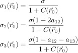
1 is the dominant local structure orientation. From {λi}, we can calculate the anisotropy values:
and their associated eigenvalues {λi}. Assuming λ1 < λ2 < λ3, n
1 is the dominant local structure orientation. From {λi}, we can calculate the anisotropy values:
| (5) |
which are used to design the kernel's standard deviations {σi}. These coefficients should be large along the main orientation of the pattern, such that the data are only smoothed in homogeneous regions and along instead of across edge surfaces. In addition, corners should be preserved during filtering. A corner is defined as the condition where the pattern is relative isotropic (a
12 ≈ 0; a
13 ≈ 0) while the local gradient strength
 is large. Therefore, a spatial dependent corner strength
 is defined as:
| (6) |
Now, we can calculate the standard deviations {σi} of the anisotropic Gaussian kernel of Eq. (3)
 |
(7) |
This anisotropic smoothing kernel is calculated for each DTI data set separately. Using this approach of Sijbers et al. [1999], the smoothing kernel width is restricted in the directions of the WM boundaries. Consequently, the volume under the kernel is reduced, which hampers the direct comparison with isotropic smoothing methods that have a larger volume under the kernel for the same FWHM. In addition, as WM structures are often very anisotropic and have a restricted width, a preservation of the kernel volume during anisotropic smoothing would lead to an overcompensation of the signal averaging along the WM structure. Therefore, this anisotropic smoothing method is implemented recursively, with a σ of 1.27 (which corresponds with a FWHM of 3 mm). In this way, WM boundaries are better preserved and an objective comparison with the isotropic approach can be made. Analogously as in the isotropic smoothing approach, the effect of the smoothing kernel width on the VBA results is evaluated by filtering the data sets with a similar range of FWHMs: 3, 6, 9, and 12 mm.
Note that, as the whole tensor is present in the simulated DTI data sets, the tensor information can be incorporated to estimate the anisotropic kernel.
Analyses of Smoothing Methods Using Simulated DTI Data Sets
The effect of smoothing on the VBA results is evaluated under perfect spatial image alignment (Analysis 1) and in the case of residual spatial misalignment, which is a more realistic situation (Analysis 2).
Analysis 1
Twenty simulated healthy and 20 pathology data sets are constructed according to the steps A–H of Figure 1. Subsequently, the FA maps of these data sets are smoothed isotropically as well as anisotropically before the statistical tests are performed in each voxel. As all images are located in atlas space, no residual image misalignment is present (see Fig. 1I).
Analysis 2
Each of the 40 DTI data sets (see Analysis 1) is now first displaced by a certain distance in a random direction. This approach of simulating image misalignment was previously described by Ashburner and Friston [2000]. In their work, misalignment was simulated as a translation of the images in a fixed direction (left‐right). To examine the effect of residual misalignment on the VBA results, the 40 DTI data sets are displaced in a randomly distributed direction by a randomly distributed distance with a mean of 2, 4, 6, and 8 mm and a standard deviation of 0.5 mm. The FA maps of the deformed data sets are subsequently smoothed and statistical tests are executed in each voxel (see Fig. 1K).
Voxel‐Wise Statistics
After filtering all the data sets with a specific smoothing method and kernel width, a nonparametric Mann‐Whitney U test is performed at every voxel to compare the FA values of the healthy and the pathology subjects [Jones et al.,2005]. In this work, only the FA is compared, because this is the diffusion measure that is most frequently reported in the literature. Although other diffusion measures can be compared analogously, they are not considered to be within the scope of this study and are therefore not included in this analysis. To reduce the chance of Type I errors, the false‐discovery rate controlling method of Benjamini and Hochberg [1995] was used to correct the P‐values for multiple comparisons [Genovese,2002]. A false‐discovery rate threshold of 0.05 was thereby applied.
Measures of VBA Accuracy
As the location, shape, and extent of the WM pathology is predefined in the simulated data sets, the VBA results can be compared quantitatively with this ground‐truth information. A measure describing the accuracy of the VBA approach is derived by counting the number of pathologies that is detected by the VBA study. If an overlap is found (independent of its size) between the predefined pathology and the VBA results, the pathology is considered to be detected.
In addition, the sensitivity and specificity of the statistical VBA results are calculated. The sensitivity is defined here as the ratio of the number of true‐positive voxels and the sum of the number of true‐positive and false‐negative voxels and the specificity is calculated as the ratio of the number of true‐negative voxels and the sum of the number of true‐negative and false‐positive voxels. A receiver‐operating characteristic (ROC) plot, displaying the true‐positive rate (TPR = sensitivity) as a function of the false‐positive rate (FPR = 1 − specificity), can then be obtained. Qualitatively, the closer the points in the ROC plot are located to the upper left corner, the higher the overall accuracy of the analysis [Zweig and Campbell,1993].
RESULTS
The Effect of Smoothing
The effect of isotropic and anisotropic smoothing on the FA is visualized for a mid‐brain axial slice intersecting the corpus callosum (Fig. 3A). As can be observed in Figure 3A, the different WM structures that can be discriminated on the original FA map are blurred after uniform, isotropic smoothing, especially for larger FWHM. In addition, the overall FA intensity of the WM decreased after isotropic smoothing due to the averaging of WM, GM, and CSF signal intensities, as is demonstrated by the FA intensity histograms of Figure 3B. In Figure 3C, the FA value is shown as a function of the amount of smoothing (for both the isotropic and anisotropic kernel) for a randomly selected voxel within several WM structures.
Figure 3.
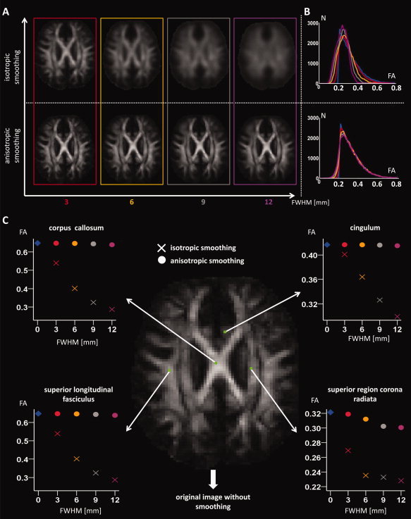
In A, an axial FA slice is shown after different levels of isotropic and anisotropic smoothing. The FA histograms after smoothing with the same kernel sizes are displayed in B. In this analysis, a WM mask (FA > 0.2) on the original image is used to only include the WM information. In C, the effect of smoothing on the FA values of different WM structures is demonstrated for a particular voxel. [Color figure can be viewed in the online issue, which is available at www.interscience.wiley.com.]
As the image boundaries are preserved during anisotropic smoothing, a filtered signal is observed in the WM, without the inclusion of GM or CSF intensities (Fig. 3A). The WM image intensities remain relatively constant after anisotropic smoothing with different kernels, as can be seen in Figure 3B,C.
Qualitative Assessment of the VBA Results
In Figure 4A,B, the VBA results of Analysis 1 are superimposed on 10 axial slices of the atlas FA map for both smoothing approaches with different smoothing kernel widths. A level of pathology corresponding with an FA decrease of 19 and 13% was used in the results of Figure 4A,B, respectively. The voxels in which ground‐truth pathology was predefined are colored in green, whereas the VBA results are colored in red. In addition, the voxels in which the VBA results and the ground‐truth pathology overlap are colored in yellow. A green, red, and yellow color in the voxels of Figure 4A,B thus represent the presence of false‐negative, false‐positive, and true‐positive results, respectively. Voxels in which the FA intensities are displayed correspond with true‐negative results. It can be observed qualitatively in Figure 4A,B that both the number of false‐positive and false‐negative results increases and the number of true‐positive results decreases for increasing isotropic smoothing kernel widths. On the other hand, a relatively high number of true‐positive results can still be observed at larger anisotropic smoothing kernel widths.
Figure 4.
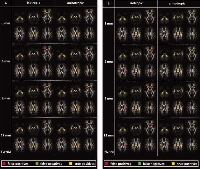
VBA results are visualized using both smoothing methods and various smoothing kernel widths. The voxels that contain a ground‐truth pathology and a significant VBA result are displayed in green and red, respectively. When both overlap, a yellow color is assigned to that voxel. False‐positive, false‐negative, and true‐positive results are therefore colored in red, green, and yellow, respectively. The voxels in which the background FA map is shown can be regarded as containing true‐negative results. A level of pathology corresponding with an FA decrease of 19 and 13% was used in the results of A and B, respectively. [Color figure can be viewed in the online issue, which is available at www.interscience.wiley.com.]
Validity of the Matched Filter Theorem
The validity of the matched filter theorem is analyzed using the simulated data sets. To this end, the FWHM that produced the highest sensitivity to detect the predefined pathology is displayed as a function of the size of this pathology, as can be seen in Figure 5. This is done for different levels of simulated tissue degradation, corresponding with an FA decrease of 10, 13, 16, and 19%. To obtain more detailed results, smoothing kernel widths from 1 to 12 mm (in steps of 1 mm) were used in this analysis. As can be observed in Figure 5, a significant correlation is found between the optimal FWHM of the anisotropic smoothing kernel and the size of the pathology. Here, the Spearman correlation coefficient ρ varies between 0.49 and 0.70 (P << 0.05). The Spearman correlation coefficient was used because the pathology size is not uniformly distributed and because the smoothing kernel widths were discretely defined. It can also be observed in Figure 5 that no correlation was found between the optimal FWHM and the size of the pathologies in the case of isotropic smoothing (a Spearman correlation coefficient ρ between 0.12 and 0.18, and a P > 0.5).
Figure 5.
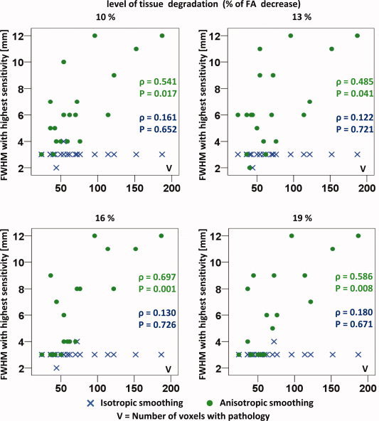
The isotropic and anisotropic smoothing kernel widths that result in the highest sensitivity for pathology detection are visualized as a function of the size of the different pathologies. This analysis is performed using different levels of tissue degradation as reflected by the averaged FA decrease. [Color figure can be viewed in the online issue, which is available at www.interscience.wiley.com.]
Percentage of Detected Pathologies
In Figure 6, the percentage of detected pathologies in the VBA analysis is displayed for different levels of simulated residual image misalignment. This analysis is performed using the two smoothing methods for a range of smoothing kernel widths. Note that the results using the largest FA decrease of 22% are displayed in Figure 6. As can be observed in the upper row of Figure 6, all pathologies were detected in the VBA analysis using anisotropic smoothing when no residual misalignment was present. The pathology detection rate decreased for an increasing level of residual misalignment, especially for the smaller lesions, as can be seen in the left column. Additionally, a lower detection rate of the pathologies was observed when the data sets were smoothed with a uniform, isotropic kernel, with a FWHM > 3 mm. In particular, the smaller pathologies were detected less frequently. The pathology detection rate after isotropic and anisotropic is smoothing compared statistically using a nonparametric Mann‐Whitney U‐test. In Figure 6, “**” denotes statistical significance at the 0.01 level.
Figure 6.

The effect of isotropic and anisotropic smoothing kernel widths on the percentage of detected pathologies is examined. In the left column, the results are displayed for the pathologies that contain <50 voxels. In the middle and the right column, the results are shown for the pathologies with a number of voxels between 50 and 65 and with a number of voxels larger than 65, respectively. In the upper row, the results of the Analysis 1 are displayed, when no residual misalignment was added to the data sets. In the second, third, and fourth row of, results are shown after displacing the data sets with a mean distance of 2, 4, and 6 mm in random directions, respectively. All results were derived for a specific level of transverse diffusivity increase, which corresponded with a mean FA decrease of 19%. [Color figure can be viewed in the online issue, which is available at www.interscience.wiley.com.]
ROC Analysis
The sensitivity and the specificity of the VBA results are displayed in an ROC graph in Figure 7 for the different smoothing approaches, various kernel widths, and different levels of pathology. In Figure 7A, an ROC plot is visualized for perfectly aligned data sets (i.e., Analysis 1). In Figure 7B–D, the true‐positive and the false‐positive rates are displayed for the simulation of different levels of residual misalignment, ranging from 2 to 6 mm.
Figure 7.
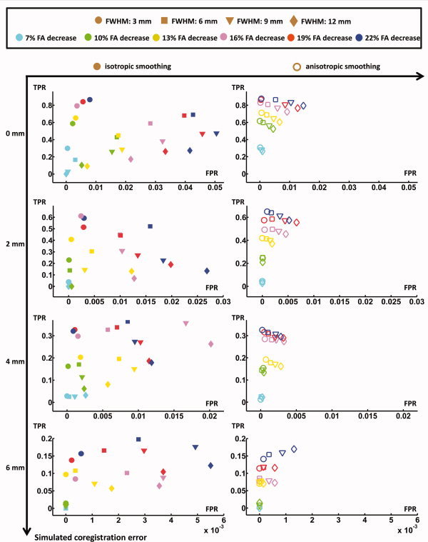
The true‐positive and false‐positive rates are displayed for VBA Analysis 1 (top left) and VBA Analysis 2 (all other plots). This is done for different isotropic and anisotropic smoothing kernel widths. [Color figure can be viewed in the online issue, which is available at www.interscience.wiley.com.]
DISCUSSION
The idea of performing a VBA of medical images originates from studies of fMRI, PET, and anatomical MR data sets [Ashburner and Friston,2001; Bookstein,2001; Fox and Mintun,2006; Fox et al.,1988; Friston et al.,1990,1991]. In recent years, this method is increasingly being applied to examine DTI data sets of subjects with various neurologic and psychiatric disorders (see Table I for an overview). In VBA, the whole brain is checked for patient‐control differences. In theory, this is a standardized method, including a coregistration of the data sets to a template and a subsequent smoothing of the transformed images. Thereafter, a voxel‐wise statistical analysis and a post‐hoc correction for multiple comparisons are performed. Although this method to analyze a group of data sets has many advantages compared with other approaches, such as the region of interest based method, recent studies suggest that the VBA results are not always accurate and standardized, because they depend on the parameter settings and implementations of the analysis [Foong et al.,2002; Jones et al.,2005,2007; Park et al.,2004; Zhang et al.,2007]. As a direct response to these issues, tract‐based spatial statistics (TBSS) was proposed by Smith et al. [2006]. In TBSS, the residual spatial misalignment is minimized by projecting the high‐FA voxels onto a subject‐mean FA tract skeleton. As a result, the number of false‐positive findings related to coregistration imperfections is reduced. However, TBSS has its own assumptions and limitations and is not always the preferred method for the analysis of DTI data sets of different subject groups. An underlying assumption of TBSS is that the pathology (or more generally, the effect of interest) occurs in voxels of WM structures where the local FA is highest (i.e., the FA skeleton), which to date has not been validated yet. As a result, only a relatively small percentage of the entire WM volume (i.e., the skeleton) is analyzed, and consequently, sensitivity is reduced. In addition, by defining the individual tract skeletons, FA values can be collapsed across different WM structures, such as, for instance, at the converging anterior segments of the fronto‐occipital fibers and the uncinate fasciculus, or the callosal fibers and the corticospinal tracts. At these positions, TBSS results can therefore not been differentiated between these anatomically different WM pathways making it difficult to draw any specific conclusions.
Note that it has been demonstrated that high‐dimensional registration algorithms that incorporate all tensor information during image alignment can reduce regional misalignments in the major WM tracts significantly. In this context, we recently demonstrated in a study of ALS patients that the use of a high‐dimensional nonaffine viscous fluid model for the registration and a population specific DTI atlas can reduce the misalignment of the DTI data sets drastically [Sage et al., in press; Van Hecke et al.,2007,2008]. In this study, it was shown that significantly improved results were found using this method compared with the SPM2 standard method. In addition, the improved VBA results were also compared with the TBSS results: both were very similar demonstrating the robustness of both techniques with respect to misalignments.
In contrast to the studies of Foong et al. [2002], Park et al. [2004], and Jones et al. [2005], in which real DTI data sets of schizophrenia patients were used where the spatial location of the underlying pathology was not known, in this work, the effect of smoothing on the VBA result is evaluated in simulated DTI data sets with a predefined pathology (i.e., a known size, shape, location, and level of FA decrease). Consequently, both sensitivity and specificity of the VBA results can be quantitatively compared between the isotropic and the anisotropic smoothing approaches.
Why Do We Smooth?
Voxel‐based methods for the analysis of fMRI and PET data rely on the assumption that all voxels are in the same anatomical reference space after coregistration and that activations are expressed in exactly the same location across subjects [Maas and Renshaw,1999]. As this assumption is not valid in practice, spatial smoothing is used to suppress the effect of functional and anatomical variability within and across subjects. This smoothing is also applied in the processing pipeline of fMRI and PET data sets to increase the SNR. In this context, the functional signal should match the hemodynamic responses, which are representative for functional activation in the brain. Worsley and Friston [1995] and Friston et al. [1996] reported that the smoothness of the images should be significantly larger than the voxel size, to ensure the underlying assumptions of the Gaussian random field theory and to match the hemodynamic response.
To date, all published DTI‐based VBA studies have applied a uniform, isotropic smoothing kernel, analogously to the analysis of fMRI and PET data sets. In addition, the rule of thumb for the smoothing kernel width that is used in the study of fMRI and PET images, that is, using a FWHM of at least two to three times the voxel dimension, is respected in almost all DTI‐based VBA studies (see Table I).
Why Should We Smooth Anisotropically?
There is no reason to assume that the implementation and parameter settings that are optimal to analyze fMRI and PET images should also be applied to examine DTI data sets. For example, in DTI, the FA value is spatially preserved along a certain spatial direction, which is determined by the WM fiber architecture. The application of an isotropic filter to DTI data sets, therefore, averages information from structured WM (high FA) with less structured tissues such as GM or CSF (low FA), as was demonstrated in Figure 3A–C.
To fulfill the requirements of the matched filter theorem in DTI, a smoothing kernel should be used that matches the size and the shape of the underlying WM pathology. Because this depends on the pathology that is studied and on the size and shape of the specific WM structure in which the pathology is situated, it is very hard to postulate a rule of thumb for the smoothing kernel width in the VBA of DT images. This is reflected by the large range of isotropic smoothing kernel widths from 0 mm to as much as 16 mm that is reported in the DTI literature (see Table I). This large variability in the smoothing kernel width across studies is particularly problematic because Foong et al. [2002], Park et al. [2004], and Jones et al. [2005] demonstrated that the reported VBA results depend on the applied smoothing kernel width.
Although the shape of the pathology is rarely known in advance, the pathology will most likely affect the WM fiber bundle, without altering the nearby CSF or GM tissue. Averaging FA values of different tissues and WM structures, as is done by isotropic smoothing, will therefore decrease the sensitivity and specificity of the pathology detection, as is shown in Figure 4. Our results suggest that isotropic smoothing leads to more false positives and that anisotropic smoothing leads to more false negatives. Moreover, in isotropic smoothing, the false positives often are isolated areas with no relation to the pathologies, whereas in anisotropic smoothing the false negatives are attached to true positives, resulting in a relatively harmless underestimation of the area affected (see Figs. 4 and 7). In this context, our results indicate that the requirements of the matched filter theorem are only satisfied when the data are filtered with an anisotropic smoothing kernel, which preserves the image boundaries (see Fig. 5). In addition, the percentage of detected pathologies decreased for an increasing FWHM of the isotropic smoothing kernel, due to the increasing contribution of voxels that are located outside the WM fiber bundle (Figs. 6 and 7).
To evaluate the effect of smoothing in the presence of coregistration inaccuracies, residual misalignment was simulated in this study. The difference in sensitivity and specificity between the smoothing approaches was lower for increasing levels of simulated residual misalignment, due to an overall decrease in the VBA sensitivity and specificity. Our results furthermore indicate that isotropic smoothing kernels can not alleviate the effect of image misalignment, as the sensitivity and specificity of the results was higher for smaller smoothing kernels in the presence of large image coregistration errors (Figs. 6 and 7). This is probably due to the severe partial volume or voxel averaging artifacts with other tissues when larger isotropic smoothing kernels were used. Obviously, it is very hard to pinpoint an optimal FWHM for smoothing in a VBA setting. On the basis of our simulated data sets, we observed that the sensitivity and specificity of pathology detection decreased for increasing smoothing kernel widths. In addition, the sensitivity and specificity of the pathology detection increased significantly when the anisotropic smoothing method was used. We therefore cautiously propose to use anisotropic smoothing methods with a FWHM of 3–6 mm.
Note that a simulated coregistration error of 4 or 6 mm (or 2–3 voxels) is much larger compared with the observed misalignment after the high‐dimensional, nonrigid image alignment of real data sets. In addition, the simulation of residual misalignment is limited because a uniform displacement is applied to every voxel of each data set, whereas in practice, misalignment is spatially dependent and thus not uniform.
CONCLUSIONS
Using simulated DTI data sets, we demonstrated that the use of anisotropic smoothing kernels can significantly increase the sensitivity and the specificity of detecting the predefined pathology in a VBA study. Our results indicate that the VBA sensitivity and specificity are significantly reduced when the data sets are smoothed isotropically with a FWHM larger than 3 mm. We therefore believe that anisotropic smoothing methods should be used in the voxel‐based DTI group analysis to increase the SNR as well as preserve the WM boundaries.
REFERENCES
- Albrecht J, Dellani PR, Mller MJ, Schermuly I, Beck M, Stoeter P, Gerhard A, Fellgiebel A ( 2007): Voxel based analyses of diffusion tensor imaging in Fabry disease. J Neurol Neurosurg Psychiatry 78: 964–969. [DOI] [PMC free article] [PubMed] [Google Scholar]
- Alexander DC, Pierpaoli C, Basser PJ, Gee JC ( 2001): Spatial transformations of diffusion tensor magnetic resonance images. IEEE Trans Med Imaging 20: 1131–1139. [DOI] [PubMed] [Google Scholar]
- Ardekani BA, Nierenberg J, Hotman MJ, Javitt DC, Lim KO ( 2003): MRI study of white matter diffusion anisotropy in schizophrenia. NeuroReport 14: 2025–2029. [DOI] [PubMed] [Google Scholar]
- Ashburner J, Friston KJ ( 2000): Voxel‐based morphometry—The methods. NeuroImage 11( 6 Part 1): 805–821. [DOI] [PubMed] [Google Scholar]
- Ashburner J, Friston KJ ( 2001): Why voxel‐based morphometry should be used. NeuroImage 14: 1238–1243. [DOI] [PubMed] [Google Scholar]
- Audoin B, Guye M, Reuter F, Au Duong MV, Confort‐Gouny S, Malikova I, Soulier E, Viout P, Chrif AA, Cozzone PJ, Pelletier J, Ranjevazz JP ( 2007): Structure of WM bundles constituting the working memory system in early multiple sclerosis: A quantitative DTI tractography study. NeuroImage 36: 1324–1330. [DOI] [PubMed] [Google Scholar]
- Barnea‐Goraly N, Eliez S, Hedeus M, Menon V, White C, Moseley M, Reiss AL ( 2003): White matter tract alterations in fragile X syndrome: Preliminary evidence from diffusion tensor imaging. Am J Med Genet B Neuropsychiatr Genet 118: 81–88. [DOI] [PubMed] [Google Scholar]
- Barnea‐Goraly N, Kwon H, Menon V, Eliez S, Lotspeich L, Reiss A ( 2004): White matter structure in autism: Preliminary evidence from diffusion tensor imaging. Biol Psychiatry 55: 323–326. [DOI] [PubMed] [Google Scholar]
- Barnea‐Goraly N, Eliez S, Menona V, Bammer R, Reiss A ( 2005): Arithmetic ability and parietal alterations: A diffusion tensor imaging study in velocardiofacial syndrome. Brain Res Cogn Brain Res 25: 735–740. [DOI] [PubMed] [Google Scholar]
- Basser PJ, Mattiello J, Le Bihan D ( 1994): MR diffusion tensor spectroscopy and imaging. Biophys J 66: 259–267. [DOI] [PMC free article] [PubMed] [Google Scholar]
- Benjamini Y, Hochberg Y ( 1995): Controlling the false discovery rate: A practical and powerful approach to multiple testing. J Roy Statist Soc Ser B 57: 289–300. [Google Scholar]
- Bookstein FL ( 2001): Voxel‐based morphometry should not be used with imperfectly registered images. NeuroImage 14: 1454–1462. [DOI] [PubMed] [Google Scholar]
- Borroni B, Brambati SM, Agosti C, Gipponi S, Bellelli G, Gasparotti R, Garibotto V, Di Luca M, Scifo P, Perani D, Padovani A ( 2007): Evidence of white matter changes on diffusion tensor imaging in frontotemporal dementia. Arch Neurol 64: 246–251. [DOI] [PubMed] [Google Scholar]
- Borroni B, Garibotto V, Agosti C, Brambati SM, Bellelli G, Gasparotti R, Padovani A, Perani D ( 2008): White matter changes in corticobasal degeneration syndrome and correlation with limb apraxia. Arch Neurol 65: 796–801. [DOI] [PubMed] [Google Scholar]
- Bruno S, Cercignani M, Ron MA ( 2008): White matter abnormalities in bipolar disorder: A voxel‐based diffusion tensor imaging study. Bipolar Disord 10: 460–468. [DOI] [PMC free article] [PubMed] [Google Scholar]
- Burns J, Job D, Bastin ME, Whalley H, Macgillivray T, Johnstone EC, Lawrie SM ( 2003): Structural disconnectivity in schizophrenia: A diffusion tensor magnetic resonance imaging study. Br J Psychiatry 182: 439–443. [PubMed] [Google Scholar]
- Ceccarelli A, Rocca MA, Pagani E, Ghezzi A, Capra R, Falini A, Scotti G, Comi G, Filippi M ( 2008): The topographical distribution of tissue injury in benign MS: A 3T multiparametric MRI study. NeuroImage 39: 1499–1509. [DOI] [PubMed] [Google Scholar]
- Cercignani M, Bozalli M, Iannucci G, Comi G, Filippi M ( 2002): Intra‐voxel and inter‐voxel coherence in patients with multiple sclerosis assessed using diffusion tensor MRI. J Neurol 249: 875–883. [DOI] [PubMed] [Google Scholar]
- Chappell MH, Ulug AM, Zhang L, Heitger MH, Jordan BD, Zimmerman RD, Watts R ( 2006): Distribution of microstructural damage in the brains of professional boxers: A diffusion MRI study. J Magn Reson Imaging 24: 537–542. [DOI] [PubMed] [Google Scholar]
- Chen B, Hsu EW ( 2005): Noise removal in magnetic resonance diffusion tensor imaging. Magn Reson Med 54: 393–407. [DOI] [PubMed] [Google Scholar]
- Ding Z, Gore JC, Anderson AW ( 2005): Reduction of noise in diffusion tensor images using anisotropic smoothing. Magn Reson Med 53: 485–490. [DOI] [PubMed] [Google Scholar]
- Erikkson SH, Rugg‐Gunn FJ, Symms MR, Barker GJ, Duncan JS ( 2001): Diffusion tensor imaging in patients with epilepsy and malformations of cortical development. Brain 124: 617–626. [DOI] [PubMed] [Google Scholar]
- Fillard P, Pennec X, Arsigny V, Ayache N ( 2007): Clinical DT‐MRI estimation, smoothing, and fiber tracking with log‐Euclidean metrics. IEEE Trans Med Imaging 26: 1472–1482. [DOI] [PubMed] [Google Scholar]
- Focke NK, Yogarajah M, Bonelli SB, Bartlett PA, Symms MR, Duncan JS ( 2008): Voxel‐based diffusion tensor imaging in patients with mesial temporal lobe epilepsy and hippocampal sclerosis. NeuroImage 40: 728–737. [DOI] [PubMed] [Google Scholar]
- Foong J, Symms MR, Barker GJ, Maier M, Miller DH, Ron MA ( 2002): Investigating regional white matter in schizophrenia using diffusion tensor imaging. NeuroReport 13: 333–336. [DOI] [PubMed] [Google Scholar]
- Fox PT, Mintun MA ( 2006): Noninvasive functional brain mapping by change‐distribution analysis of averaged PET images of H2 15 O tissue activity. J Nucl Med 30: 141–149. [PubMed] [Google Scholar]
- Fox PT, Mintun MA, Reiman EM, Raichle ME ( 1988): Enhanced detection of focal brain responses using intersubject averaging and change‐distribution analysis of subtracted PET images. J Cereb Blood Flow Metab 8: 642–653. [DOI] [PubMed] [Google Scholar]
- Friston KJ, Frith CD, Liddle PF, Dolan RJ, Lammertsmaa AA, Frackowiak RSJ ( 1990): The relationship between global and local changes in PET scans. J Cereb Blood Flow Metab 13: 1038–1040. [DOI] [PubMed] [Google Scholar]
- Friston KJ, Frith CD, Liddle PF, Frackowiak RSJ ( 1991): Comparing functional (PET) images: The assessment of significant change. J Cereb Blood Flow Metab 11: 690–699. [DOI] [PubMed] [Google Scholar]
- Friston KJ, Holmes A, Poline J‐B, Price CJ, Frith CD ( 1996): Detecting activations in PET and fMRI: Levels of inference and power. NeuroImage 4: 223–235. [DOI] [PubMed] [Google Scholar]
- Ge Y, Law M, Johnson G, Herbert J, Babb JS, Mannon LJ, Grossman RI ( 2004): Preferential occult injury of corpus callosum in multiple sclerosis measured by diffusion tensor imaging. J Magn Reson Imaging 20: 1–7. [DOI] [PubMed] [Google Scholar]
- Genovese CR, Lazar NA, Nichols T ( 2002): Thresholding of statistical maps in functional neuroimaging using the false discovery rate. NeuroImage 15: 870–878. [DOI] [PubMed] [Google Scholar]
- Gimenez M, Miranda MJ, Born AP, Nagy Z, Rostrup E, Jernigan TL ( 2008): Accelerated cerebral white matter development in preterm infants: A voxel‐based morphometry study with diffusion tensor MR imaging. NeuroImage 41: 728–734. [DOI] [PubMed] [Google Scholar]
- Golestani N, Molko N, Dehaene S. an LeBihan D, Pallier C ( 2007): Brain structure predicts the learning of foreign speech sounds. Cereb Cortex 17: 575–582. [DOI] [PubMed] [Google Scholar]
- Hasan KM, Gupta RK, Santos RM, Wolinsky JS, Narayana PA ( 2005): Fractional diffusion tensor anisotropy of the seven segments of the normal‐appearing white matter of the corpus callosum in healthy adults and relapsing remitting multiple sclerosis. J Magn Reson Imaging 21: 735–743. [DOI] [PubMed] [Google Scholar]
- Holzapfel M, Barnea‐Goraly N, Eckert MA, Kesler SR, Reiss AL ( 2006): Selective alterations of white matter associated with visuospatial and sensorimotor dysfunction in turner syndrome. J Neurosci 26: 7007–7013. [DOI] [PMC free article] [PubMed] [Google Scholar]
- Jones DK ( 2004): The effect of gradient sampling schemes on measures derived from diffusion tensor MRI: A Monte Carlo study. Magn Reson Med 51: 807–815. [DOI] [PubMed] [Google Scholar]
- Jones DK, Griffin LD, Alexander DC, Catani M, Horsfield MA, Howard R, Williams SCR ( 2002): Spatial normalization and averaging of diffusion tensor MRI data sets. NeuroImage 17: 592–617. [PubMed] [Google Scholar]
- Jones DK, Symms MR, Cercignani M, Howarde RJ ( 2005): The effect of filter size on VBM analyses of DT‐MRI data. NeuroImage 26: 546–554. [DOI] [PubMed] [Google Scholar]
- Jones DK, Chitnis XA, Job D, Khong PL, Leung LT, Marenco S, Smith SM, Symms MR ( 2007): What happens when nine different groups analyze the same DT‐MRI data set using voxel‐based methods? In: Proceedings of the 15th Annual Meeting of the ISMRM, Berlin. p. 74.
- Kumar R, Gupta RK, Elderkin‐Thompson V, Huda A, Sayre J, Kirsch C, Guze B, Han S, Thomas MA ( 2006): Voxel‐based diffusion tensor magnetic resonance imaging evaluation of low‐grade hepatic encephalopathy. J Magn Reson Imaging 27: 1061–1068. [DOI] [PubMed] [Google Scholar]
- Kyriakopoulos M, Vyas NS, Barker GJ, Chitnis XA, Frangou S ( 2007): A diffusion tensor imaging study of white matter in early‐onset schizophrenia. Biol Psychiatry 63: 519–523. [DOI] [PubMed] [Google Scholar]
- Lee JE, Chung MK, Lazar M, DuBray MB, Kim J, Bigler ED, Lainhart JE, Alexander AL ( 2009): A study of diffusion tensor imaging by tissue‐specific, smoothing‐compensated voxel‐based analysis. NeuroImage 44: 870–883. [DOI] [PMC free article] [PubMed] [Google Scholar]
- Leemans A, Sijbers J, De Backer S, Vandervliet E, Parizel PM ( 2005): Affine coregistration of diffusion tensor magnetic resonance images using mutual information. Lect Notes Comput Sci 3708: 523–530. [Google Scholar]
- Leemans A, Jones DK ( 2009): The B‐matrix must be rotated when correcting for subject motion in DTI data. Magn Reson 61: 1336–1349. [DOI] [PubMed] [Google Scholar]
- Leemans A, Jeurissen B, Sijbers J, Jones D ( 2009): ExploreDTI: A graphical toolbox for processing, analyzing, and visualizing diffusion MR data. In: Proceedings of the 17th Annual Meeting of International Society of Magnetic Resonance Medicine, Hawaii. p. 3537.
- Li C, Sun X, Zou K, Yang H, Huang X, Wang Y, Lui S, Li D, Zou L, Chen H ( 2007): Voxel based Analysis of DTI in depression patients. Int J Magn Reson Imaging 1: 43–48. [Google Scholar]
- Maas LC, Renshaw, PF ( 1999): Post‐registration spatial filtering to reduce noise in functional MRI data sets. Magn Reson Imaging 17: 1371–1382. [DOI] [PubMed] [Google Scholar]
- Maes F, Collignon A, Vandermeulen D, Marchal G, Suetens P ( 1997): Multimodality image registration by maximization of mutual information. IEEE Trans Med Imaging 16: 187–198. [DOI] [PubMed] [Google Scholar]
- Martin‐Fernandez M, Muñoz‐Moreno E, Cammoun L, Thiran J‐P, Westin C‐F, Alberola López C ( 2009): Sequential anisotropic multichannel Wiener filtering with Rician bias correction applied to 3D regularization of DWI data. Med Image Analysis 13: 19–35. [DOI] [PMC free article] [PubMed] [Google Scholar]
- Menzies L, Williams GB, Chamberlain SR, Ooi C, Fineberg N, Suckling J, Sahakian BJ, Robbins TW, Bullmore ET ( 2008): White matter abnormalities in patients with obsessive—Compulsive disorder and their first‐degree relatives. Am J Psychiatry 165: 1308–1315. [DOI] [PubMed] [Google Scholar]
- Molko N, Cachia A, Riviere D, Mangin J‐F, Bruandet M, Le Bihan D, Cohen L, Dehaene S ( 2004): Brain anatomy in turner syndrome: Evidence for impaired social and spatial‐numerical networks. Cereb Cortex 14: 840–850. [DOI] [PubMed] [Google Scholar]
- Nagy Z, Westerberg H, Skare S, Andersson JL, Lilja A, Flodmark O, Fernell E, Holmberg K, Bohm B, Forssberg H, Lagercrantz H, Klingberg T ( 2003): Preterm children have disturbances of white matter at 11 years of age as shown by diffusion tensor imaging. Pediatr Res 54: 672–679. [DOI] [PubMed] [Google Scholar]
- Ng M‐C, Ho JT, Ho S‐L, Lee R, Li G, Cheng T‐S, Song Y‐Q, Ho PW‐L, Fong GC‐Y, Mak W, Chan K‐H, Li LS‐W, Luk KD‐K, Hu Y, Ramsden DB, Leong LL‐Y ( 2008): Abnormal diffusion tensor in nonsymptomatic familial amyotrophic lateral sclerosis with a causative superoxide dismutase 1 mutation. J Magn Reson Imaging 27: 8–13. [DOI] [PubMed] [Google Scholar]
- Oh J, Henry RG, Genain C, Nelson SJ, Pelletier D ( 2004): Mechanisms of normal appearing corpus callosum injury related to pericallosal T1 lesions in multiple sclerosis using directional diffusion tensor and 1H MRS imaging. J Neurol Neurosurg Psychiatry 75: 1281–1286. [DOI] [PMC free article] [PubMed] [Google Scholar]
- Padovani A, Borroni B, Brambati SM, Agosti C, Broli M, Alonso R, Scifo P, Bellelli G, Alberici A, Gasparotti R, Perani D ( 2005): Diffusion tensor imaging and voxel based morphometry study in early progressive supranuclear palsy. J Neurol Neurosurg Psychiatry 77: 457–463. [DOI] [PMC free article] [PubMed] [Google Scholar]
- Pagani E, Agosta F, Rocca MA, Caputo D, Filippi M ( 2008): Voxel‐based analysis derived from fractional anisotropy images of white matter volume changes with aging. NeuroImage 41: 657–667. [DOI] [PubMed] [Google Scholar]
- Park H‐J, Westin C‐F, Kubicki M, Maier SE, Niznikiewicz M, Baer A, Frumin M, Kikinis R, Jolesz FA, McCarley RW, Shenton ME ( 2004): White matter hemisphere asymmetries in healthy subjects and in schizophrenia: A diffusion tensor MRI study. NeuroImage 23: 213–223. [DOI] [PMC free article] [PubMed] [Google Scholar]
- Perona P, Malik J ( 1990): Scale‐space and edge detection using anisotropic diffusion. IEEE Trans Pattern Anal Mach Intell 12: 629–639. [Google Scholar]
- Petersson KM, Nichols TE, Poline JB, Holmes AP ( 1999): Statistical limitations in functional neuroimaging II. Signal detection and statistical inference. Philos Trans R Soc Lond B Biol Sci 354: 1261–1281. [DOI] [PMC free article] [PubMed] [Google Scholar]
- Porto L, Preibisch C, Hattingen E, Bartels M, Lehrnbecher T, Dewitz R, Zanella F, Good C, Lanfermann H, DuMesnil R, Kieslich M ( 2008): Voxel‐based morphometry and diffusion‐tensor MR imaging of the brain in long‐term survivors of childhood leukemia. Eur J Radiol 18: 2691–2700. [DOI] [PubMed] [Google Scholar]
- Rose SE, Janke AL, Chalk JB ( 2008): Gray and white matter changes in Alzheimers disease: A diffusion tensor imaging study. J Magn Reson Imaging 27: 20–26. [DOI] [PubMed] [Google Scholar]
- Rosenfeld A, Kak AC ( 1982): Digital Picture Processing 2. Orlando FL: Academic Press. [Google Scholar]
- Sach M, Winkler G, Glauche V, Liepert J, Heimbach B, Koch MA, Bchel C, Weiller C ( 2004): Diffusion tensor MRI of early upper motor neuron involvement in amyotrophic lateral sclerosis. Brain 127: 340–350. [DOI] [PubMed] [Google Scholar]
- Sage CAS, Peeters RR, Grner A, Robberecht W, Sunaert S ( 2007): Quantitative diffusion tensor imaging in amyotrophic lateral sclerosis. NeuroImage 34: 486–499. [DOI] [PubMed] [Google Scholar]
- Sage CA, Van Hecke W, Peeters R, Sijbers J, Robberecht W, Parizel PM, Marchal G, Leemans A, Sunaert S: Quantitative diffusion tensor imaging in amyotrophic lateral sclerosis: Revisited (in press). [DOI] [PMC free article] [PubMed]
- Seok JH, Park HJ, Chun JW, Lee SK, Cho HS, Kwon JS, Kim JJ ( 2007): White matter abnormalities associated with auditory hallucinations in schizophrenia: A combined study of voxel‐based analyses of diffusion tensor imaging and structural magnetic resonance imaging. Psychiatry Res 156: 93–104. [DOI] [PubMed] [Google Scholar]
- Shergill S, Kanaan R, Chitnis XA, ODaly O, Jones D, Frangou S, Williams SCR, Howard RJ ( 2007): A diffusion tensor imaging study of fasciculi in schizophrenia. Am J Psychiatry 164: 467–473. [DOI] [PubMed] [Google Scholar]
- Shin Y, Kwon J, Ha T, Park H, Kim D, Hong S, Moon W, Lee J, Kim I, Kim S, Chung E ( 2006): Increased water diffusivity in the frontal and temporal cortices of schizophrenic patients. NeuroImage 30: 1285–1291. [DOI] [PubMed] [Google Scholar]
- Sijbers J, den Dekker A, Verhoye M, Van der Linden A, Van Dyck D ( 1999): Adaptive anisotropic noise filtering for magnitude MR data. Magn Reson Imaging 17: 1533–1539. [DOI] [PubMed] [Google Scholar]
- Skelly LR, Calhoun V, Meda SA, Kim J, Mathalon DHS, Pearlson GD ( 2008): Diffusion tensor imaging in schizophrenia: Relationship to symptoms. Schizophr Res 98: 157–162. [DOI] [PMC free article] [PubMed] [Google Scholar]
- Smith SM, Jenkinson M, Johansen‐Berg H, Rueckert D, Nichols TE, Mackay CE, Watkins KE, Ciccarelli O, Cader MZ, Matthews PMS, Behrens TE ( 2006): Tract‐based spatial statistics: Voxelwise analysis of multi‐subject diffusion data. NeuroImage 4: 1487–1505. [DOI] [PubMed] [Google Scholar]
- Snook L, Plewes C, Beaulieu C ( 2007): Voxel based versus region of interest analysis in diffusion tensor imaging of neurodevelopment. NeuroImage 34: 243–252. [DOI] [PubMed] [Google Scholar]
- Thivard L, Pradat P‐F, Leh'ericy S, Lacomblez L, Dormont D, Chiras J, Benali H, Meininger V ( 2007): Diffusion tensor imaging and voxel‐based morphometry study in amyotrophic lateral sclerosis: Relationships with motor disability. J Neurol Neurosurg Psychiatry 78: 889–892. [DOI] [PMC free article] [PubMed] [Google Scholar]
- Van Hecke W, Leemans A, D'Agostino E, De Backer S, Vandervliet E, Parizel PM, Sijbers J ( 2007): Nonrigid coregistration of diffusion tensor images using a viscous fluid model and mutual information. IEEE Trans Med Imaging 26: 1598–1612. [DOI] [PubMed] [Google Scholar]
- Van Hecke W, Leemans A, D'Agostino E, Maes F, De Backer S, Vandervliet E, Sijbers J, Parizel PM ( 2008): On the construction of an inter‐subject diffusion tensor magnetic resonance atlas of the healthy human brain. NeuroImage 43: 69–80. [DOI] [PubMed] [Google Scholar]
- Van Hecke W, Sijbers J, De Backer S, Poot D, Parizel PM, Leemans A ( 2009): On the construction of a ground‐truth framework for evaluating voxel‐based diffusion tensor MRI analysis methods. NeuroImage 46: 692–707. [DOI] [PubMed] [Google Scholar]
- Vangberg TR, Skranes J, Dale AM, Martinussen M, Brubakk A‐M, Haraldseth O ( 2006): Changes in white matter diffusion anisotropy in adolescents born prematurely. NeuroImage 32: 1538–1548. [DOI] [PubMed] [Google Scholar]
- White T, Kendi ATK, Lehricy S, Kendi M, Karatekin C, Guimaraes A, Davenport N, Schulz SC, Lim KO ( 2007): Disruption of hippocampal connectivity in children and adolescents with schizophrenia—A voxel‐based diffusion tensor imaging study. Schizophr Res 90: 302–307. [DOI] [PubMed] [Google Scholar]
- Worsley KJ, Evans AC, Marrett S, Neelin P ( 1992): A three‐dimensional statistical analysis for CBF activation studies in human brain. J Cereb Blood Flow Metab 12: 900–918. [DOI] [PubMed] [Google Scholar]
- Worsley KJ, Friston KJ ( 1995): Analysis of fMRI time‐series revisited‐again. Neuroimage 2: 173–181. [DOI] [PubMed] [Google Scholar]
- Yu CS, Zhu CZ, Li KC, Xuan Y, Qin W, Sun H, Chan P ( 2007): Relapsing neuromyelitis optica and relapsing‐remitting multiple sclerosis: Differentiation at diffusion‐tensor MR imaging of corpus callosum. Radiology 244: 249–256. [DOI] [PubMed] [Google Scholar]
- Zhang H, Avants BB, Yushkevich PA, Woo JH, Wang S, McCluskey LF, Elman LB, Melhem ER, Gee JC ( 2007): High‐dimensional spatial normalization of diffusion tensor images improves the detection of white matter differences: An example study using amyotrophic lateral sclerosis. IEEE Trans Med Imaging 26: 1585–1597. [DOI] [PubMed] [Google Scholar]
- Zweig MH, Campbell G ( 1993): Receiver‐operating characteristic (ROC) plots: A fundamental evaluation tool in clinical medicine. Clin Chem 39: 561–577. [PubMed] [Google Scholar]