

Abstract
A number of techniques have been used to provide functional connectivity estimates for a given fMRI data set. In this study we compared two methods: a ‘rest‐like’ method where the functional connectivity was estimated for the whitened residuals after regressing out the task‐induced effects, and a within‐condition method where the functional connectivity was estimated separately for each experimental condition. In both cases four pre‐processing strategies were used: 1) time courses extracted from standard pre‐processed data (standard); 2) adjusted time courses extracted using the volume of interest routines in SPM2 from standard pre‐processed data (spm); 3) time courses extracted from ICA denoised data (standard denoised); and 4) adjusted time courses extracted from ICA denoised data (spm denoised). The temporal correlation between time series extracted from two cortical regions were statistically compared with the temporal correlation between a time series extracted from a cortical region and a time series extracted form a region placed in CSF. Since the later correlation is due to physiological noise and other artifacts, we used this comparison to investigate whether rest‐like and task modulated connectivity could be estimated from the same data set. The pre‐processing strategy had a significant effect on the connectivity estimates with the standard time courses providing larger connectivity values than the spm time courses for both estimation methods. The CSF comparison indicated that for our data set only rest‐like connectivity could be estimated. The rest‐like connectivity values were similar with connectivity estimated from resting state data. Hum Brain Mapp 2008. © 2007 Wiley‐Liss, Inc.
Keywords: functional connectivity, time course selection, ICA denoising
INTRODUCTION
Functional connectivity has been defined as the “temporal correlation between spatially separated neurophysiological measurements” [Friston et al.,1993a]. In the case of functional magnetic resonance imaging (fMRI), estimates of functional connectivity are derived from correlations between series of scans that measure the flow of oxygenated blood in the brain at discrete time intervals. Measures of functional connectivity can be augmented with a model of directional influences within a given network to estimate effective connectivity, defined as “the influence one neuronal system exerts over another” [Friston et al.,1993b]. Effective connectivity in fMRI data can be estimated by applying anatomical constraints prior to structural equation modeling [Bullmore et al.,2000; Gavrilescu et al.,2004; Gonçalves and Hall,2003; McIntosh and Gonzales‐Lima,1994], or by exploiting the temporal relationships between the correlated time series [Abler et al.,2006; Sato et al.,2006]. Alternatively, dynamic causal modelling [Friston et al.,2003; Mechelli et al., 2004] has been used to measure the modulatory influence of activity in one brain region on the functional connectivity between other pairs of regions. In all these methods, accurate estimation of functional connectivity is an important prerequisite for estimation of effective connectivity.
Although various estimates of functional connectivity have been used to characterize the functional integration of different brain areas, at present there is no consensus regarding the definition and measurement of this construct [Horwitz,2003; Lee et al.,2003]. There are several factors contributing to this situation. First, functional connectivity is assumed to originate in the correlated firing rates of a network of interconnected neurons. Since fMRI data are measures of changes in metabolism via the blood oxygenation level‐dependent (BOLD) signal, a proper characterization of functional connectivity in the fMRI data depends upon our understanding of the mechanisms that relate neuronal level activity with the metabolic changes. Many aspects of these mechanisms have yet to be elucidated [Leopold et al.,2003; Logothetis et al.,2001]. This means that it is not clear which aspect of the correlation between fMRI time series reflects underlying neuronal connectivity. Specifically, there is a lack of agreement regarding which temporal components of the correlation between two fMRI time series are most relevant to the estimation of functional connectivity. While many studies have implicated the low frequency components of time series correlations [Cordes et al.,2000; Lowe et al.,2000; Xiong et al.,1999], others have isolated correlated components at the highest temporal frequencies, represented by changes in activation between successive scans [Horwitz,1991].
The estimation of functional connectivity in fMRI studies using activation tasks presents additional problems, since the general definition of functional connectivity does not distinguish between inter‐regional correlations due to a common response to the external task, and correlations between other components of a time series that are not associated with the task. Functional connectivity has been estimated in these data sets by keeping the task‐induced responses within the time series [Bullmore et al.,2000; Whalley et al.,2005]. However, it has been argued that since task‐dependent relationships may usefully be characterized as “co‐activation,” they do not necessarily imply any connection between two regions [Lowe et al.,1998]. In the extreme case, common input from distal sense organs alone may generate similar responses in disparate brain regions. Accordingly, strategies have been developed to remove the task‐related variance from fMRI time series and use the residual variance to estimate a rest‐like connectivity [Arfanakis et al.,2000; Fair et al.,2007]. Moreover, separate inter‐regional correlation matrices can be derived for each experimental condition (within‐condition functional connectivity) to study modulation in connectivity induced by the tasks under study [Büchel and Friston,1997; Gonçalves and Hall,2003; Honey et al.,2002,2003; Maguire et al.,2000; Rogers et al.,2004; Schlösser et al.,2003, Kondo et al.,2004]. In principle, it should be possible to use the same data set to estimate both correlated spontaneous fluctuations in BOLD signal (rest‐like connectivity) and the modulation in these fluctuations induced by the task under study.
Finally, a major source of variation between studies arises from differences in data preprocessing prior to connectivity analysis. These include temporal filtering, spatial smoothing, representative time course selection, and artifact removal. The fMRI noise can have two opposite effects on functional connectivity estimation. The temporal correlation between two time courses can be spuriously increased or decreased depending on the similarity of drifts, head motion, and contributions from the physiological noise across the investigated regions. Therefore, the choice of preprocessing parameters is very important in the context of functional connectivity estimation, since it determines how the fMRI signal divides into useful signal and noise. With so many different parameters and preprocessing implementations to choose from, it is very likely that the measured connectivity depends upon the preprocessing strategy, and it may be very difficult to select an optimal strategy for a given data set. To summarize, when confronted with functional connectivity estimation for a particular data set, the researcher is asked to choose between a multitude of operational definitions of functional connectivity that differ both conceptually and in the details of implementation. To our knowledge, there is at present no objective justification for the selection of a particular functional connectivity estimation method or of a particular preprocessing strategy. This selection is of particular importance for studies comparing connectivity estimates across groups of participants (e.g., between patients and healthy controls), since in this case, it is expected that the spatial and temporal patterns of variance are different across groups and these differences can contaminate the observed connectivity differences.
The problem is further complicated by the fact that the effects of preprocessing strategy cannot be interpreted based solely on comparing the estimated correlation values across strategies, since, depending on the nature of the modeled noise, the estimated correlation values can either increase or decrease. In this study, we used a simple statistical comparison to help with this selection. Cordes et al. [2001] convincingly demonstrated that the temporal correlations of a seed region placed in CSF with the rest of the brain were driven by physiological noise. We have compared the correlation estimated between time series extracted from two cortical regions against the correlation estimated between a time series extracted from a cortical region with a time series extracted from a region placed in CSF. Further, we have employed the CSF comparison to investigate whether both rest‐like and task modulation in connectivity could be estimated from the same task activation data set. If both methods would provide significantly higher cortico‐cortical than cortico‐CSF correlation values, we can conclude that both connectivity types are estimable form the same data set. This would be an important finding, since it can reduce the fMRI scanning time. Usually, a “localizer” functional run with a simple relevant task needs to be used to identify the ROIs for resting state connectivity and then data from another functional run with a more complex paradigm is used to investigate the modulation of connectivity by the experimental manipulations.
The aim of this study is two‐fold: (i) to investigate if indeed the choice of preprocessing strategy has a significant impact on functional connectivity estimates and (ii) to explore whether rest‐like connectivity and task‐induced modulation in connectivity can be estimated from the same task activation data set. The data set used to explore these issues came from a study of interhemispheric functional connectivity between the secondary auditory cortices.
METHODS
Data Description
Seven healthy subjects (average age 37 ± 8.6, four females) with no history of neurological deficits were scanned while passively listening to semantically neutral words. Gradient echo planar images were recorded using a 3T G.E. Signa LX whole body scanner with the following imaging parameters: TR = 3 s, TE = 40 ms, FA = 60, FOV = 24 cm; 128 × 128 matrix with 1.88 × 1.88 mm2 in plane resolution; 25 trans‐axial slices 4.5 mm thick with 0.5 mm gap. Two scanning sessions were acquired for each participant. The word stimuli were presented as a block design with three active conditions and a resting state baseline. All four conditions were presented in each block. While the baseline condition was always placed at the end of the block, the order of the active conditions was pseudo‐randomized across blocks using a Latin square design (see Fig. 2). During the active conditions, semantically neutral words were presented to the subjects either monaurally (to the left or to the right ear) or binaurally. The stimuli were presented using electrodynamic speakers compatible with the MRI environment [Baumgart et al.,1998; http://www.mr-confon.de]. The mean duration of the words was 516 ms, and they were adjusted to produce equal loudness. Six words were presented per condition with an interstimulus interval of ∼1 s (the total duration of each condition was 9 s allowing the acquisition of three full brain images). The duration of the rest condition was also 9 s. Data was acquired for 14 blocks per subject (seven blocks per session). The subjects were instructed to relax with their eyes closed and listen to the stimuli.
Figure 2.
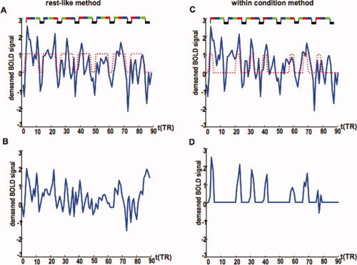
The functional connectivity estimation methods. For simplicity, only one session is represented. The rest‐like method: (A) The demeaned time courses extracted from A2R in one subject. A delayed box‐car model (2 × TR) is superposed on the time course (dotted line). The experimental paradigm is represented at the top of the panel; each condition lasted for 9 s (3 × TR) and is represented by a different color: red‐binaural presentation; blue‐left ear presentation; green‐right ear presentation; black‐baseline. (B) The residual time course after the stimulus induced response estimated as the average across the seven blocks in (A) was regressed out. The within‐condition method: (C) The demeaned time course extracted from A2R in one subject with the delayed box‐car regressor for the binaural condition represented by the dotted line. (D) The time points corresponding to the binaural condition extracted from the time course in (C). Prior to connectivity estimation, the first volume in each block was discarded and the remaining time points were concatenated to create the time course corresponding to the binaural condition. The time courses corresponding to the left and right ear presentation were estimated in a similar way. [Color figure can be viewed in the online issue, which is available at www.interscience.wiley.com.]
Preprocessing Strategies for Time Course Extraction
The images from all subjects were motion‐corrected using a rigid body six degrees of freedom transformation in SPM2. To explore the impact of preprocessing strategies on the functional connectivity estimation, we compared the results based on time courses extracted from images after spatial normalization and spatial smoothing (classic preprocessed data), with those based on time courses extracted from images after applying an ICA‐based denoising procedure (denoised data). In principle, ICA can identify imaging artifacts produced by ghosting, slice drop out, and B0 effects that may contaminate temporal correlation values. These artifacts are difficult to identify based on simple image inspection.
We created the denoised data set by performing a spatial independent components analysis (ICA) for each subject, using the ICA as implemented in Melodic2 (http://www.fmrib.ox.ac.uk/fsl/melodic). An effective data denoising requires as a first step the identification of the task‐induced effects. The task‐related components were identified by ranking the components after the correlation with the experimental paradigm [Esposito et al.,2002] and after the number of activated voxels in the regions of interest [Esposito et al.,2003]. All the temporal courses and associated spatial patterns were visually inspected to identify artifacts (slice drop‐outs, gradient instability, EPI ghost, high frequency noise, head motion, B0 field inhomogeneity, eye‐related artifacts, spin history artifacts). The components that were significantly correlated with the motion parameters [r > 0.5, Van de Ven et al.,2004] and had spatial patterns around the brain edges, as well as components expressing strong temporal drifts, or other identified artifacts were then removed from the data by projecting the data set onto the remaining components.
The two data sets (original and denoised data) were then preprocessed in a similar manner using SPM2 (http://www.fil.ion.ucl.ac.uk/spm/). For each subject, the images were normalized to the EPI template, interpolated to a resolution of 2 × 2 × 2 mm3, and spatially smoothed using an 8 × 8 × 8 mm3 Gaussian kernel. In this way, we obtained two preprocessed data sets: standard preprocessed data (motion correction followed by spatial normalization and spatial smoothing) and denoised data (motion correction followed by ICA denoising, spatial normalization, and spatial smoothing).
We extracted the time courses for both standard and denoised data in the relevant regions of interest (ROIs) in two ways: (1) based on SPM2 volume of interest (VOI) extraction routine (spm time courses) and (2) by extracting the same voxel values directly from the images used for analysis (standard time courses). The spm time courses were adjusted for the effects of interest, and for serial correlation via an autoregressive model of order one [AR(1)] model; the representative time course was then calculated as the first eigenvariate of a singular value decomposition across the voxels. The standard time courses were mean‐centered, variance‐normalized, and high pass‐filtered to remove the contributions from extremely low frequencies (frequencies < 0.01 Hz), since fMRI data are prone to artifacts in this frequency range [Cordes and Nandy,2003]. The same routine used for high pass‐filtering in SPM2 (based on discrete cosine transform basis functions) was employed to filter the standard time courses. Mean centering and variance normalization were applied within session and the time courses were concatenated across the two sessions. The representative time course was then calculated by averaging all time courses in a given region of interest.
The combination of two data sets (standard and denoised) with two time course extraction methods (standard and spm time course) provided us with four preprocessing strategies for time course extraction: (1) standard extracted time courses (standard); (2) spm‐extracted time courses (spm); (3) standard time courses extracted from denoised data (standard denoised), and (4) spm time courses extracted from denoised data (spm denoised).
The statistical significance of the differences in the correlation values produced by using different preprocessing strategies was assessed using a one‐way repeated measures ANOVA analysis on the left secondary auditory cortex (A2L) to right secondary auditory cortex (A2R) correlation values.
Regions of Interest
The statistical analysis of both standard and denoised data sets was performed using SPM2 by employing a high pass temporal filter with 100 s cut off and an AR(1) model to account for temporal autocorrelation in the data.
For the two data sets, we selected the ROIs based on the SPM2 F‐maps of the effects of interest at P < 0.001, uncorrected probability threshold. We identified for each subject, 4 mm radius spherical ROIs over the secondary auditory cortex (see Fig. 1A) both in the left (A2L) and the right (A2R) hemispheres. The center of each region was selected based on visual inspection of the SPM F‐maps, rather than automatically selecting the voxel with the highest statistical score, to avoid placing the center of the sphere at the border of the ROI.
Figure 1.
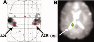
(A) The SPM2 F map of the effects of interest for one subject (P < 0.001, uncorrected probability threshold). The red circles indicate the placement of ROIs and the arrows indicate the secondary auditory cortices. (B) The CSF region defined manually using MRIcro. [Color figure can be viewed in the online issue, which is available at www.interscience.wiley.com.]
Functional Connectivity Estimation
We estimated the functional connectivity in two ways. Firstly, we estimated a rest‐like functional connectivity based on calculating the correlation coefficient (r) between residuals after the task effects were removed from the data. The task‐induced effects were identified by averaging the representative time course of a given ROI within the blocks of task presentation. To account for the hemodynamic delay, we shifted each block by 6 s (2 × TR) and we performed an average across sessions (14 blocks, see Fig. 2A,B). The task effects were estimated separately for each region and for each subject to take into account intersubject variability as well as within subject spatial variations in the hemodynamic response as suggested by Handwerker et al. [2004]. The task effect was then regressed out from the representative time course of each region and functional connectivity was estimated as the correlation between the residuals.
The power spectra of the spm regressors for the left, right, and binaural condition, and of the sum of these three regressors had peaks in the frequency intervals 0.02–0.04 Hz, 0.05–0.06 Hz, and 0.07–0.08 Hz. The sum of the areas under the graph for these three frequency intervals was estimated from the power spectra of the original time courses before the task effects were regressed out. This sum was also estimated for the time courses after the task effects were regressed out. The statistical comparison of these areas enabled us to assess whether indeed our method was effective in removing the task‐induced effect.
In addition, we compared the rest‐like connectivity estimates with functional connectivity estimated from the resting state data (TR = 2 s; matrix 64 × 64 with 3 × 3 mm2 in plane resolution; 25 trans‐axial slices 4.5 mm with 0.5 mm gap; FOV = 24 cm; FA = 60; 146 images/subject) for the same ROIs. Resting state data were available for five subjects and we performed this comparison for the standard preprocessed data. After motion correction, the resting state data were coregistered with the motion‐corrected task activation data and smoothed with a 5 × 5 × 5 mm3 Gaussian kernel. The coordinates of ROIs defined in the spatially normalized task activation data were then projected back to the native space to allow the use of the same ROI coordinates in the resting state data.
Secondly, we estimated a within‐condition functional connectivity. The representative time courses for each region, and each subject, were split into conditions after applying a temporal shift of 6 s (2 × TR) to account for the hemodynamic delay (Fig. 2C,D). The block segments were then concatenated within each region to form three time courses for the stimulus presented to the left ear (left), stimulus presented to the right ear (right), and stimulus presented binaurally (binaural), respectively. To minimize the effects of the hemodynamic delay at the block edges [Homae et al.,2003], we also discarded the first time point from each block leaving 28 time points per condition for each subject and each region. The connectivity corresponding to the baseline condition was not estimated, since the duration of this condition is shorter than the BOLD undershoot.
Statistical Comparison of the Cortico‐Cortical Correlation With the Cortico‐CSF Correlation
To compare the performance of the two functional connectivity estimation methods, we implemented a simple statistical comparison of the estimated correlation between A2L and A2R with the correlation between A2L and a region defined in CSF (left lateral ventricle). Cordes et al. [2001] have shown that CSF‐cortical temporal correlations have major contributions from respiratory and cardiac noise. Thus, a significant increase in cortico‐cortical temporal correlation relative to CSF‐cortical correlation would indicate that the cortico‐cortical correlation originates from other sources; and may in principle represent true functional connectivity provided that these cortical areas are indeed functionally connected.
The CSF region was manually defined (see Fig. 1B) for each subject using MRIcro software (http://www.psychology.nottingham.ac.uk/staff/cr1/mricro.html). The time course preprocessing methods and the functional connectivity methods were applied identically for the CSF region.
The correlation between the A2L and A2R regions and the correlation between the A2L with CSF regions were compared using an appropriate statistical test [Williams' t test, Williams,1959, see Appendix A] that accounts for the interdependency of this comparison (A2L is a common area in both correlation). An important assumption is that the Williams' t requires independent observations. Therefore, we investigated the temporal autocorrelation function to test for independence. Since SPM2 analysis employed an AR(1) model, we expect the spm time courses to demonstrate nonsignificant autocorrelation. For the standard time courses, we have applied vector autoregressive models (VAR, see Appendix B) to create noncorrelated residuals. Given our method to construct the within‐condition time courses (only two images from each condition were selected), we do not expect the temporal autocorrelation to be significant for these time courses.
Group Level Statistical Test
To assess the significance of the validity test at the group level, we have employed a statistical approach that takes into account the scan level variance (via Williams' t) and the hierarchical structure of the data. Williams' t values were combined at the group level to calculate a group Z statistic based on a meta‐analytic approach according to Winer [1971]
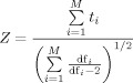 |
where M is the number of subjects and df represents the degrees of freedom for the Williams' t, df = N − 3, where N is the number of scans. The Z score calculated based on the Winer formula also requires independent observations. This approach combines the probability at the group level and has been demonstrated to provide superior power characteristics [McNamee and Lazar,2004; Rosenthal,1991].
RESULTS
Statistical Analysis and Region of Interest Selection
The word stimuli produced statistically significant BOLD activation in the auditory cortices for all investigated subjects (see Fig. 1A for an example of an individual F‐map) allowing us to define the ROIs based on the individual functional maps. The coordinates of the ROIs (from the effects of interest maps, p < 0.001, uncorrected) were in the range of coordinates previously reported for A2 [Griffiths and Warren,2002].
Time Courses Whitening
As expected, the within‐condition time courses demonstrated autocorrelation values within 95% confidence interval for all preprocessing strategies. For six out of seven subjects, the autocorrelation values for the spm time courses were also nonsignificant. However, one subject (subject no. 3) demonstrated significantly large autocorrelation values for all three regions (A2L, A2R, and CSF) both for standard and denoised data. An AR(4) model rendered white residuals for this subject. Table I shows the values of AR coefficients for lag j = 1 as estimated in SPM2 for the standard preprocessed data. In SPM2, the AR model is estimated globally across all voxels identified as activated during the first pass [Friston et al.,2002]. Therefore, SPM2 employs the same AR coefficients across all voxels for a given subject (i.e., the spm time courses for A2L and A2R were whitened using the same A 1 coefficient).
Table I.
The AR and VAR coefficients across subjects (lag j = 1)
| Subject | SPM2 (AR) | VAR | |||
|---|---|---|---|---|---|
| A2L | A2R | ||||
| A 1 | A 1 | B 1 | A 1 | B 1 | |
| 1 | 0.37 | 0.30 | 0.09 | 0.08 | 0.30 |
| 2 | 0.20 | 0.31 | −0.20 | −0.03 | 0.12 |
| 3a | 0.37 | 0.78 | −0.29 | 0.74 | −0.37 |
| 4 | 0.26 | 0.42 | 0.17 | 0.02 | 0.62 |
| 5 | 0.37 | 0.61 | 0.02 | 0.20 | 0.45 |
| 6 | 0.37 | 0.39 | 0.30 | 0.17 | 0.24 |
| 7 | 0.37 | 0.22 | 0.13 | −0.02 | 0.26 |
Subject no. 3 needed an order 4 model to provide white residuals both for spm and standard preproccesed time courses. The A 1 coefficients when using an AR(4) model for the spm time courses of this subject were 0.5198 for A2L and 0.5173 for A2R. The VAR coefficients included in the table for subject no. 3 were estimated using an VAR(4) model.
A VAR(1) model produced white residuals for the standard time courses in all subjects, except subject no. 3, where a VAR(4) model was used to obtain white residuals. The corresponding Williams' t test values were calculated taking into account that four degrees of freedom were lost for a VAR(1) model, while the VAR(4) model for subject no. 3 implied the loss of 10 degrees of freedom (see Appendix B). Table I shows the values of the VAR coefficients for the standard preprocessed data (A and B coefficients in relations B1 and B2, see Appendix B) for lag j = 1. The VAR coefficients were estimated separately for A2L and A2R.
Task Removal Efficiency
The area under the graph, corresponding to the three intervals where the task regressors exhibited peaks, was measured in the power spectra of the original time course before the task effects were regressed out. This area was then remeasured in the residual time courses after the task‐induced effects were regressed out. Statistical comparison of these areas was based on separate 2 way ANOVAs for A2L and A2R (factors: task removal with two levels before and after; and preprocessing strategy with four levels). For both regions, the contributions to the power spectra at the stimulus frequency was significantly reduced after task removal (F 1,48 = 12.9, p < 0.0001 for A2L; F 1,48 = 15.95, p < 0.0001 for A2R) showing that the task effects were effectively removed.
The comparison of the rest‐like and resting state estimates for A2L to A2R connectivity across five subjects showed that these estimates were not significantly different: r rest‐like = 0.49 ± 0.06, r resting state = 0.48 ± 0.15, p = 0.9.
The Preprocessing Effects on Functional Connectivity Estimates
ICA decomposition identified for our data set components showing extremely low frequency drifts (<0.01 Hz), strong correlation with the motion parameters, slice drop out, and components with large number of voxels in areas susceptible to B0 artifacts. These components were removed from the data by projecting the data set onto the remaining component.
For the rest‐like connectivity estimation, the one‐way ANOVA (factor: preprocessing strategy with four levels) indicated a significant preprocessing effect (F 3,24 = 4.40, p = 0.01) with the correlation coefficients for the standard classic time courses significantly larger than those for the spm time courses. The standard denoised time courses also yielded significantly larger correlations than the spm time courses both with standard and denoised data (Fig. 3A).
Figure 3.
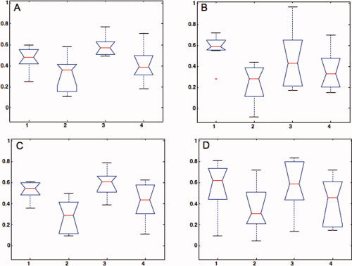
The box plots of the functional connectivity estimates across preprocessing strategies. (A) rest‐like method; (B) within‐condition method, left ear presentation; (C) within‐condition method, right ear presentation; (D) within‐condition method, binaural presentation; 1, standard preprocessing; 2, spm preprocessing; 3, standard denoised preprocessing; 4, spm denoised preprocessing. [Color figure can be viewed in the online issue, which is available at www.interscience. wiley.com.]
The connectivity estimates based on the within‐condition method were investigated for significant preprocessing effects with separated one‐way ANOVAs for each active condition. For the left ear presentation condition, the one‐way ANOVA indicated again a significant preprocessing effect (F 3,24 = 3.31, p = 0.04), with standard time courses providing significantly larger correlation coefficients than spm time courses both with standard and denoised data (Fig. 3B). For the right ear presentation, the effect of preprocessing strategy was significant (F 3,24 = 6.49, p = 0.002) with spm time courses giving significantly lower correlation coefficients than the standard time courses for both standard and denoised data (Fig. 3C). A similar trend was obtained for the binaural condition, the effect was however, not significant (F 3,24 = 1.54, p = 0.200, see Fig. 3D).
In summary, the preprocessing strategy had a significant impact on the connectivity estimates. The standard time courses gave significantly larger connectivity values than the spm extracted time courses, and data denoising showed no significant effect over the standard preprocessing.
Statistical Comparison of the Cortico‐Cortical Correlation With the Cortico‐CSF Correlation
The two methods of functional connectivity estimation differed markedly when we statistically compared the cortico‐cortical connectivity with the cortico‐CSF connectivity.
The rest‐like method produced significantly higher group level correlation values for A2L‐A2R correlation than for A2L‐CSF correlation for all preprocessing strategies with a very small number of subjects showing not significant results (see Table II).
Table II.
Williams' t test values for the statistical comparison between A2L‐A2R and A2L‐CSF correlation
| Subject | The “rest‐like” method | |||
|---|---|---|---|---|
| Standard | spm | Standard denoised | spm denoised | |
| 1 | 5.24 (<0.0001) | 3.91 (0.0003) | 5.85 (<0.0001) | 3.39 (0.0015) |
| 2 | 6.57 (<0.0001) | 3.70 (0.0005) | 6.04 (<0.0001) | 5.46 (<0.0001) |
| 3 | 7.85 (<0.0001) | 8.00 (<0.0001) | 10.42 (<0.0001) | 8.53 (<0.0001) |
| 4 | 6.10 (<0.0001) | 5.10 (<0.0001) | 6.46 (<0.0001) | 4.96 (<0.0001) |
| 5 | 6.13 (<0.0001) | 3.26 (0.0022) | 3.07 (0.0039) | 3.63 (0.0001) |
| 6 | 1.82 (0.0766) | 0.81 (0.2867) | 8.20 (<0.0001) | 5.40 (<0.0001) |
| 7 | 5.08 (<0.0001) | 4.10 (0.0001) | 4.70 (<0.0001) | 1.78 (0.0828) |
| Group level | 5.47 (∼ 10−7) | 4.10 (∼ 10−4) | 6.31 (∼ 10−10) | 4.67 (∼ 10−6) |
The correlation values were estimated using the rest‐like method. The values in brackets represent the associated probability values.
The within‐condition functional connectivity estimation method produced significant group level results only for the standard time courses (see Table II for left ear presentation condition; similar results were obtained for right ear and binaural presentation). None of the individual subjects had significant t values for the spm time courses (Table III). In general, the individual subject t values were markedly lower than for the residuals method. No consistent pattern of variance in connectivity values with the stimulus laterality was observed across subjects for the within‐condition method with any preprocessing strategy.
Table III.
Williams' t test values for the statistical comparison between A2L‐A2R and A2L‐CSF correlation
| Subject | The within‐condition method | |||
|---|---|---|---|---|
| Standard | spm | Standard denoised | spm denoised | |
| 1 | 3.20 (0.0045) | 1.54 (0.1211) | 3.05 (0.0065) | 0.85 (0.2728) |
| 2 | 0.99 (0.2385) | 0.82 (0.2797) | 1.42 (0.1434) | 1.55 (0.1203) |
| 3 | 1.42 (0.1434) | 1.43 (0.1422) | 3.16 (0.0050) | 1.43 (0.1423) |
| 4 | 2.58 (0.0184) | 1.45 (0.1378) | 2.72 (0.0135) | 2.00 (0.0585) |
| 5 | 4.60 (0.0001) | 1.64 (0.1040) | 2.77 (0.0122) | 3.35 (0.0032) |
| 6 | 1.40 (0.1511) | −0.55 (0.3377) | 4.55 (0.0002) | 2.36 (0.0287) |
| 7 | 2.52 (0.0209) | 0.39 (0.3649) | 3.22 (0.0043) | 1.16 (0.1990) |
| Group level | 2.19 (0.0359) | 0.88 (0.2698) | 2.75 (0.0092) | 1.67 (0.0993) |
The correlation values were estimated using the within‐condition method and the values correspond to the left ear stimulus presentation. The values in brackets represent the associated probability values.
Group level statistical values (Winer's Z) were generally slightly higher for the standard time courses when compared with the spm time courses and also for the denoised data compared with standard preprocessing. At the subject level data denoising had variable effects. For example, in Table II, subject no. 6 had not significant t values for the standard data, whilst data denoising rendering the t values for this subject as highly significant. However, the t test for subject no. 7 became not significant for the spm time courses after denoising, although this subject had a significant t value without denoising.
All the validity tests were repeated comparing A2L‐A2R correlation to A2R‐CSF correlation with similar results.
DISCUSSION
We investigated whether data preprocessing had a significant impact on the functional connectivity estimates in a task activation data set. To achieve this, we calculated the correlation coefficient between time courses extracted from left and right secondary auditory cortices from an fMRI data set preprocessed in four different ways. We have also explored the estimation of rest‐like and task‐induced connectivity modulation in the same task activation data set. The correlation coefficients were estimated by regressing out the task‐induced responses and correlating the residuals (rest‐like method) or separately for each experimental condition (within‐condition method).
Regarding the preprocessing effects, our results showed that, in general, the preprocessing strategy had a significant effect on the functional connectivity estimates regardless of the estimation method. The time courses extracted directly from images (standard time courses) provided significantly higher correlation coefficients than the time courses extracted via the VOI routine in SPM2 (spm time courses).
Taking into account the way we implemented the standard time course extraction and preprocessing, there are two sources of difference between the standard and the spm time courses. Firstly, for the spm time courses, the representative time course of a ROI was calculated as the first eigenvariate across all voxels in the ROI. For the standard time courses, the representative time course was calculated as the average across all voxels. Secondly, the whitening procedure varied between the two preprocessing strategies. The spm time courses were whitened using the same AR coefficients for all voxels for a given subject (see Table I). These coefficients are estimated globally across all voxels identified as activated during the first pass [Friston et al.,2002]. For the standard preprocessed time courses, we sought to provide optimal whitening for two given time courses at a time, and we effectively used different whitening parameters for each time course (see Table I). Moreover, we accounted for any variance in one time course that might have been explained by the signal history of the other (via B coefficients in relations B1 and B2, see Appendix B). Thus, we estimated only the instantaneous influence between A2L and A2R. This instantaneous influence between two regions is one of the measures estimated by Goebel et al. [2003]. In this study, we were not interested in estimating the Granger causality between areas, as estimated in Goebel et al. [2003]. We did not expect any difference in directional correlations from A2L to A2R as compared to A2R to A2L at the temporal resolution of our data (TR = 3 s).
It is very likely that the observed significant difference in our study between the connectivity estimated using spm and standard time courses is generated from a combination of these effects. Since the standard preprocessed time courses provided significantly larger connectivity estimates (see Fig. 3) associated with slightly larger Williams' t values (Table II), we can conclude that the standard preprocessing was more effective in removing noise‐induced variance that was not similar across A2L and A2R time courses. The implementation of our VAR method for brain level connectivity might be computationally time‐consuming but is useful for a smaller network of regions.
For our data set, the ICA‐based data denoising had no significant effect on connectivity estimates, although the correlation coefficients for the denoised time courses were slightly larger than those without denoising. This result suggests that for the data set under study, the removed artifacts were not temporally similar across the ROIs. It is worth mentioning that, in principle, removing ICA identified noise can decrease the correlation values when these artifacts have similar temporal patterns across the investigated brain regions. Therefore, the denoising results are expected to be data set‐dependent. An important observation is that the use of ICA for data denoising is highly subjective and time‐demanding, since the ultimate components classification is based on visual inspection and depends upon the experience of the investigator. Although Melodic2 employs an objective method to estimate dimensionality [Beckmann and Smith,2004], the components pertaining to each subject still need to be inspected and classified.
Our second aim was to investigate whether rest‐like and task‐modulated connectivity were estimable from the same task activation data. The statistical comparison of cortico‐cortical correlation with cortico‐CSF correlation helped us to differentiate between the two functional connectivity estimation methods. While the rest‐like method provided significantly larger cortico‐cortical correlations for all preprocessing strategies, the within‐condition method yielded significant results only for the standard time courses. These two estimation methods target different sources of functional connectivity and have different applications; therefore, we do not want to imply that the within‐condition method is incorrect. For certain data sets and experimental designs, the estimation of task‐induced modulation in connectivity might, however, not be possible.
The resting state connectivity originates from the spontaneous firing of interconnected neurons [Xiong et al.,1999]. A similar connectivity measure can be estimated from active task data sets under the assumption that the task‐induced effects can be effectively removed from the data. Our study and previous research [Arfanakis et al.,2000; Fair et al.,2007; Whalley et al.,2005] indicated that the removal of the task‐related effects can be effectively implemented for block design data. A direct comparison between rest‐like and resting state connectivity can demonstrate that indeed the spontaneous correlated fluctuations in the BOLD signal (as measured by resting state connectivity) can be recovered from task activation data. For our study, the resting state and rest‐like connectivity estimates were similar suggesting that the rest‐like functional connectivity estimation method was successful in capturing the spontaneous fluctuation in the BOLD signal for the data set under study.
The estimation of rest‐like connectivity from task activation data as implemented in this study and in previous studies [Arfanakis et al.,2000; Fair et al.,2007; Whalley et al.,2005] is, however, based on the assumption of a linear superposition of task‐related and spontaneous fluctuations in the BOLD signal. Recently, Fox et al. [2006] demonstrated the linearity of this superposition for the motor cortex. Moreover, Fair et al. [2007] indicated that the studies published so far support this hypothesis for primary sensory and motor regions. The assumption of linearity might not hold, however, for different brain areas, or for different experimental designs [Fair et al.,2007]. The direct comparison of the rest‐like connectivity estimated from task activation data sets with the connectivity estimated for the same ROIs in resting state data can help in assessing the validity of the linearity assumption for a given data set.
In principle, ICA may improve the removal of the task‐induced effects as used by Arfanakis et al. [2000], although the inclusion of this approach is beyond the scope of the current study. Note that methods based on the entire time courses, such as the residuals method, have the advantage of using all the temporal information, and can lead to functional connectivity measures that take into account the signal history as proposed by Lahaye et al. [2003] and Sato et al. [2006].
The within‐condition method can be used to investigate the changes induced in connectivity by experimental manipulation and is therefore of great importance in neuroimaging research. McIntosh [1999] suggested that this is the preferred functional connectivity estimation method in studies aiming to investigate effective connectivity with SEM.
We found no statistically significant differences between cortico‐cortical and cortico‐CSF correlation values estimated using the within‐condition method. Since only two time points per block were used to estimate the within‐condition connectivity, it is expected that this limited our sensitivity in detecting the task modulation effects. The similarity of cortico‐cortical and cortico‐CSF correlations for the within‐condition method is therefore likely to reflect the fact that the noise‐related variance in the split time courses was similar for A2L, A2R, and CSF regions.
The performance of the within‐condition method is expected to be task‐dependent and it would be appropriate for some experimental designs. For example, tasks having longer baseline and active conditions will have relatively less signal superposition from one condition to another due to the hemodynamic delay, such that the BOLD signal in each condition can reach a steady state. Skudlarski et al. [2000] found that the correlations between contralateral brain areas in motor, auditory, and visual cortices measured in short resting state or active conditions time series (35 s) were similar with those obtained for very long time series (up to 2,500 images). Moreover, Fair et al. [2007] concluded that the connectivity estimated for the rest condition between blocks of active task (after accounting for BOLD undershoot) was very similar to the connectivity estimated from continuous resting state scanning. Therefore, based on our results and previously published studies, it can be concluded that reliable connectivity values can be estimated from block design data by splitting the time series in segments corresponding to different experimental conditions under the strict assumption that these segments are long enough to account for the overlap of BOLD signal increase to the steady state value (around 10 s, Fair et al.,2007] and the undershoot at the end of an active block (around 15 s, Fair et al.,2007].
For the within‐condition functional connectivity estimation, it is also very important to investigate the stability of the experimentally induced modulation on connectivity across subjects. If indeed experimental manipulation had a significant impact on connectivity, this modulation effect should be similar across subjects. In our study, the influence of stimulus laterality on connectivity was highly variable across subjects and preprocessing strategy‐dependent, further suggesting that the within‐condition method was not appropriate for our data.
The statistical comparison of cortico‐cortical and cortico‐CSF correlation is important, since the physiological noise and imaging artifacts (signal drifts) may provide spurious sources of temporal correlation [Lund,2001]. Since Cordes et al. [2001] found that CSF connectivity is driven mostly by physiological noise, our finding of a significantly higher correlation value between A2L and A2R indicates that this relative increase in correlation has to come from a different source. Moreover, the same study found that physiological noise makes a negligible contribution (less than 10%) to auditory cortex connectivity. Although in our data the physiological noise components are likely to be aliased (our TR = 3 s), it is unlikely that the A2L to A2R correlation was driven entirely by physiological noise, since there is strong evidence in the literature that these two areas are functionally connected. The auditory cortices are anatomically connected by transcallosal fibers crossing at the level of splenium [Huang et al.,2005]. Resting state connectivity studies have reported functional interhemispheric connectivity for the auditory areas [Cordes et al.,2000]. Moreover, Cordes et al. [2001] showed that the physiological noise had only a modest contribution (less than 10%) to the connectivity maps associated with cortical areas (motor, visual, auditory). For exploratory studies where no a priori evidence of functional connectivity exists, we suggest that a better way to deal with physiological noise contamination would be to use a shorter TR or to effectively remove the contributions from physiological noise prior to connectivity estimation. This can be achieved either by regressing the physiological noise measured during fMRI scanning [Peltier and Noll,2002] or as estimated from the data [Lund and Hanson,2001].
An important assumption when comparing cortico‐cortical to cortico‐CSF correlation values is that similar correlation values are not uniformly distributed across the brain, but that higher correlation values are observed only for brain regions that are functionally connected. In our data, large correlation values were not observed across the whole brain.
Other brain regions (such as a region placed over a major vein or artery) can be used to test the validity of functional connectivity estimation. In this study, we used a region in the lateral ventricle since this region is very easy to identify in a T2* image.
In conclusion, our results indicated that functional connectivity estimation significantly depends upon the preprocessing strategy. The time courses extracted directly from the spatially normalized images were characterized by significantly larger correlation values. Furthermore, this study suggests that comparing the connectivity between two cortical areas with the CSF connectivity may be a valuable tool to investigate what type of functional connectivity is estimable from a given data set. For our data set, only the rest‐like connectivity was statistically estimable.
Acknowledgements
We express our gratitude to the three anonymous reviewers whose comments significantly improved the manuscript.
APPENDIX A.
Let X 1, X 2, and X 3 be three variable (e.g., three time courses). Williams' t test [Williams,1959] can be used to statistically compare the correlation coefficient r 1 between X 1 and X 2 with the correlation coefficient r 2 between X 1 and X 3 (Fig. A1).
Figure A1.
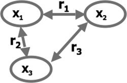
Schematic representation of the correlation coefficients compared using Williams' t test. In this study, we have compared the correlation between A2L and A2R (r 1) with the correlation between A2L and CSF (r 2).
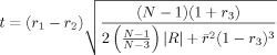
Williams' t test is defined as
 |
(A1) |
where R is calculated as the determinant of the correlation matrix
 |
(A2) |
and r 2 is the square of the r 1 and r 2 average value
| (A3) |
The Williams' t test requires independent observations. N represents the sample size. The corresponding probability value can be calculated based on the probability distribution function of the Student's t test with N − 3 degrees of freedom.
Hittner and Silver [2003] performed a Monte Carlo simulation to compare different statistical tests for dependent correlations and concluded that Williams' t test had optimal power and type I error rate.
APPENDIX B.
We have employed vector autoregressive lagged regression models to render the observation independent. For the estimation of the correlation coefficient r between two time courses X(t) and Y(t), an order i vector autoregressive model [VAR(i)] was first fitted to each time course [Gujarati,1995]
| (B1) |
| (B2) |
where Ax, Ay, Bx, and By are the regression coefficients, Cx and Cy are constant terms, and Ex and Ey are the residuals. Note that terms Y(t) and X(t) were not included in the right side of Eqs. (B1) and (B2), respectively. Therefore, the instantaneous influence between X and Y [Goebel et al.,2003] can be estimated as the correlation of the residuals Ex and Ey.
We have fitted these models using least square linear regression and estimated the residuals Ex(t) and Ey(t). The fit of an VAR(i) implies a reduction in the number of degrees of freedom from N to N − (2i + 2) for each time course.
REFERENCES
- Abler B,Roebroeck A,Goebel R,Hose A,Schonfeldt‐Lecuona C,Hole G,Walter H ( 2006): Investigating directed influences between activated brain areas in a motor‐response task using fMRI. Magn Reson Imaging 24: 181–185. [DOI] [PubMed] [Google Scholar]
- Arfanakis K,Cordes D,Haughton VM,Moritz CH,Quigley MA,Meyerand ME ( 2000): Combining independent component analysis and correlation analysis to probe interregional connectivity in fMRI task activation datasets. Magn Reson Imaging 18: 921–930. [DOI] [PubMed] [Google Scholar]
- Baumgart F,Kaulisch T,Tempelmann C,Gauschler‐Marfeski B,Tegeler C,Schindler F,Stiller D,Scheich H ( 1998): Electrodynamic headphones and woofers for application in magnetic resonance imaging scanners. Med Phys 25: 2068–2069. [DOI] [PubMed] [Google Scholar]
- Beckmann C,Smith SM ( 2004): Probabilistic independent component analysis for functional magnetic resonance imaging. IEEE Trans Med Imaging 23: 137–152. [DOI] [PubMed] [Google Scholar]
- Büchel C,Friston KJ ( 1997): Modulation of connectivity in visual pathways by attention: Cortical interactions evaluated with structural equation modelling and fMRI. Cereb Cortex 7: 768–778. [DOI] [PubMed] [Google Scholar]
- Bullmore E,Horwitz B,Honey G,Brammer M,Williams S,Sharma T ( 2000): How good is good enough in path analysis of fMRI data? NeuroImage 11: 289–301. [DOI] [PubMed] [Google Scholar]
- Cordes D,Nandy R ( 2003): Investigating the frequency dependence of spatial gradient artifacts for the analysis of resting‐state fMRI data. Presented at the 9th International Conference on Functional Mapping of the Human Brain,June 18–22, 2003, New York. Available on CD‐Rom in NeuroImage Vol. 19, No. 2.
- Cordes D,Haughton VM,Arfanakis K,Wendt GJ,Turski PA,Moritz CH,Quigley MA,Meyerand ME ( 2000): Mapping functionally related regions of brain with functional connectivity MR imaging. Am J Neuroradiol 21: 1636–1644. [PMC free article] [PubMed] [Google Scholar]
- Cordes D,Haughton VM,Arfanakis K,Carew JD,Turski PA,Moritz CH,Quigley MA,Meyerand ME ( 2001): Frequencies contribution to functional connectivity in cerebral cortex in “resting‐state” data. Am J Neuroradiol 22: 1326–1333. [PMC free article] [PubMed] [Google Scholar]
- Esposito F,Formisano E,Seifritz E,Goebel R,Morrone R,Tedeschi G,Di Salle F ( 2002): Spatial independent component analysis of functional MRI time‐series: To what extent do results depend on the algorithm used? Hum Brain Mapp 16: 146–157. [DOI] [PMC free article] [PubMed] [Google Scholar]
- Esposito F,Seifritz E,Formisano E,Morrone R,Scarabino T,Tedeschi G,Cirillo S,Goebel R,Di Salle F ( 2003): Real‐time independent component analysis of fMRI time‐series. Neuroimage 20: 2209–2224. [DOI] [PubMed] [Google Scholar]
- Fair DA,Schlaggar BL,Cohen AL,Miezin FM,Dosenbach NUF,Wenger KK,Fox MD,Snyder AZ,Raichle ME,Petersen SE ( 2007): A method for using blocked and event‐related fMRI data to study “resting state” functional connectivity. NeuroImage 35: 396–405. [DOI] [PMC free article] [PubMed] [Google Scholar]
- Fox MD,Snyder AZ,Zacks JM,Raichle ME ( 2006): Coherent spontaneous activity accounts for trial‐to‐trial variability in human evoked brain responses. Nat Neurosci 9: 23–25. [DOI] [PubMed] [Google Scholar]
- Friston KJ,Frith CD,Liddle PF,Frackowiak RSJ ( 1993a): Functional connectivity: The principal component analysis of large (PET) data sets. J Cereb Blood Flow Metab 13: 5–14. [DOI] [PubMed] [Google Scholar]
- Friston KJ,Frith CD,Frackowiak RSJ ( 1993b): Time‐dependent changes in effective connectivity measured with PET. Hum Brain Mapp 1: 69–80. [Google Scholar]
- Friston KJ,Glaser DE,Henson RN,Kiebel S,Phillips C,Ashburner J ( 2002): Classical and Bayesian inference in neuroimaging: Applications. NeuroImage 16: 484–512. [DOI] [PubMed] [Google Scholar]
- Friston KJ,Harrison L,Penny W ( 2003): Dynamic causal modeling. Neuroimage 19: 1273–1302. [DOI] [PubMed] [Google Scholar]
- Gavrilescu M,Stuart WG,Waites A,Jackson G,Svalbe ID,Egan GF ( 2004): Changes in effective connectivity models in the presence of task correlated motion: An fMRI study. Hum Brain Mapp 29: 49–63. [DOI] [PMC free article] [PubMed] [Google Scholar]
- Goebel R,Roebroeck A,Kimb D‐S,Formisano E ( 2003): Investigating directed cortical interactions in time‐resolved fMRI data using vector autoregressive modeling and Granger causality mapping. Magn Reson Imag 21: 1251–1261. [DOI] [PubMed] [Google Scholar]
- Gonçalves MS,Hall DA ( 2003): Connectivity analysis with structural equation modelling: An example of the effects of voxel selection. Neuroimage 20: 1455–1467. [DOI] [PubMed] [Google Scholar]
- Griffiths TD,Warren JD ( 2002): The planum temporale as a computational hub. Trends Neurosci 25: 348–353. [DOI] [PubMed] [Google Scholar]
- Gujarati DN ( 1995): Basic Econometrics. New York: McGraw‐Hill. [Google Scholar]
- Handwerker DA,Ollinger JM,D'Esposito M ( 2004): Variation of BOLD hemodynamic responses across subjects and brain regions and their effects on statistical analyses. Neuroimage 21: 1639–1651. [DOI] [PubMed] [Google Scholar]
- Hittner JB,Silver NC ( 2003): A Monte Carlo evaluation of test for comparing dependent correlations. J Gen Psychol 130: 149–168. [DOI] [PubMed] [Google Scholar]
- Homae F,Yahata N,Sakai LK ( 2003): Selective enhancement of functional connectivity in the left prefrontal cortex during sentence processing. Neuroimage 20: 578–586. [DOI] [PubMed] [Google Scholar]
- Honey GD,Fu CHY,Kim J,Brammer MJ,Croudace TJ,Suckling J,Pich EM,Williams SCR,Bullmore ET ( 2002): Effects of verbal working memory load on corticocortical connectivity modeled by path analysis of functional magnetic resonance imaging data. Neuroimage 17: 573–582. [PubMed] [Google Scholar]
- Honey GD,Suckling J,Zelaya F,Long C,Routledge C,Jackson S,Ng V,Fletcher PC,Williams SCR,Brown J,Bullmore ET ( 2003): Dopaminergic drug effects on physiological connectivity in a human cortico‐striato‐thalamic system. Brain 126: 1767–1781. [DOI] [PMC free article] [PubMed] [Google Scholar]
- Horwitz B ( 1991): Functional interactions in the brain: Use of correlation between regional metabolic rates. J Cereb Blood Flow Metab 11: A114–A120. [DOI] [PubMed] [Google Scholar]
- Horwitz B ( 2003): The elusive concept of brain connectivity. Neuroimage 19: 466–470. [DOI] [PubMed] [Google Scholar]
- Huang H,Zhang J,Jiang H,Wakana S,Poetscher L,Miller MI,van Zijl PCM,Hillis AE,Wytik R,Mori S ( 2005): DTI tractography based parcellation of white matter: Application to the mid‐sagittal morphology of corpus callosum. NeuroImage 26: 195–205. [DOI] [PubMed] [Google Scholar]
- Kondo H,Morishita M,Osaka N,Osaka M,Fukuyama H,Shibasaki H ( 2004): Functional roles of the cingulo‐frontal network in performance on working memory. Neuroimage 21: 2–14. [DOI] [PubMed] [Google Scholar]
- Lahaye P‐J,Poline J‐B,Flandin G,Dodel S,Garnero L ( 2003): Functional connectivity: Studying nonlinear, delayed interactions between BOLD signals. Neuroimage 20: 962–974. [DOI] [PubMed] [Google Scholar]
- Lee L,Harrison LM,Mechelli A ( 2003): A report of the functional connectivity workshop, Dusseldorf 2002. Neuroimage 19: 457–465. [DOI] [PubMed] [Google Scholar]
- Leopold DA,Murayama Y,Logothetis NK ( 2003): Very slow activity fluctuations in monkey visual cortex: Implications for functional brain imaging. Cereb Cortex 13: 422–433. [DOI] [PubMed] [Google Scholar]
- Logothetis NK,Pauls J,Augath M,Trinath T,Oeltermann A ( 2001): Neurophysiological investigation of the basis of the fMRI signal. Nature 412: 150–157. [DOI] [PubMed] [Google Scholar]
- Lowe MJ,Mock BJ,Sorenson JA ( 1998): Functional connectivity in single and multislice echoplanar imaging using resting‐state fluctuations. Neuroimage 7: 119–132. [DOI] [PubMed] [Google Scholar]
- Lowe MJ,Dzemidzic M,Lurito JT,Mathews VP,Phillips MD ( 2000): Correlations in low‐frequency BOLD fluctuations reflect cortico‐cortical connections. Neuroimage 12: 582–587. [DOI] [PubMed] [Google Scholar]
- Lund TE ( 2001): fcMRI‐mapping functional connectivity or correlating cardiac‐induced noise? Magn Reson Med 46: 628–629. [DOI] [PubMed] [Google Scholar]
- Lund TE,Hanson LG ( 2001): Physiological noise correction in fMRI using vessel time‐series as covariates in a general linear model. In: Proceedings of the 9th Annual Meeting of ISMRM. p 22.
- Maguire EA,Mummery CJ,Büchel C ( 2000): Patterns of hippocampal cortical interaction dissociate temporal lobe memory subsystems. Hippocampus 10: 475–482. [DOI] [PubMed] [Google Scholar]
- McIntosh AR ( 1999): Mapping cognition to the brain through neural interactions. Memory 7: 523–548. [DOI] [PubMed] [Google Scholar]
- McIntosh AR,Gonzales‐Lima F ( 1994): Structural equation modeling and its application to network analysis in functional brain imaging. Human Brain Mapping 2: 2–22. [Google Scholar]
- McNamee RL,Lazar NA ( 2004): Assessing the sensitivity of fMRI group maps. Neuroimage 22: 920–931. [DOI] [PubMed] [Google Scholar]
- Mechelli A,Price CJ,Noppeney U,Friston KJ ( 2003): A dynamic causal modeling study on category effects: Bottom–up or top–down mediation? J Cogn Neurosci 15: 925–934. [DOI] [PubMed] [Google Scholar]
- Peltier SJ,Noll DC ( 2002): T2 * dependence of low frequency functional connectivity. Neuroimage 16: 985–992. [DOI] [PubMed] [Google Scholar]
- Rogers BP,Carew JD,Meyerand ME ( 2004): Hemispheric asymmetry in supplementary motor area connectivity during unilateral finger movements. Neuroimage 22: 855–859. [DOI] [PubMed] [Google Scholar]
- Rosenthal R ( 1991): Meta‐analytic procedures for social research (revised edition). Newbury Park,CA: Sage; p 90. [Google Scholar]
- Sato JR,Amaro Junior E,Takahashi DY,de Maria Felix M,Brammer MJ,Morettin PA ( 2006): A method to produce evolving functional connectivity maps during the course of an fMRI experiment using wavelet‐based time‐varying Granger causality. Neuroimage 31: 187–189. [DOI] [PubMed] [Google Scholar]
- Schlösser R,Gesierich T,Kaufmann B,Vucurevic G,Hunsche S,Gawehn J,Stoeter P ( 2003): Altered effective connectivity during working memory performance in schizophrenia: A study with fMRI and structural equation modeling. Neuroimage 19: 751–763. [DOI] [PubMed] [Google Scholar]
- Skudlarski P,Wexler B,Fulbright R,Gore J ( 2000): Inter‐regional correlations in the fMRI time‐course evident in short imaging series. Neuroimage 11: S549. [Google Scholar]
- Van de Ven VG,Formisano E,Prvulovic D,Roeder CH,Linden DEJ ( 2004): Functional connectivity as revealed by spatial independent component analysis of fMRI measurements during rest. Human Brain Mapping 22: 165–178. [DOI] [PMC free article] [PubMed] [Google Scholar]
- Williams EJ ( 1959): The comparison of regression variables. J R Stat Soc Ser B 21: 396–399. [Google Scholar]
- Winer BJ ( 1971): Statistical principles in experimental design, 2nd ed. New York: McGRaw Hill. [Google Scholar]
- Whalley HC,Simonotto E,Marshall I,Owens DG,Goddard NH,Johnstone EC,Lawrie SM ( 2005): Functional disconnectivity in subjects at high genetic risk of schizophrenia. Brain 128: 2097–2108. [DOI] [PubMed] [Google Scholar]
- Xiong J,Parsons L M, Gao J,Fox PT ( 1999): Interregional connectivity to primary motor cortex revealed using MRI resting state images. Hum Brain Mapp 8: 151–156. [DOI] [PMC free article] [PubMed] [Google Scholar]