Assessing and minimizing the effects of noise and motion in clinical DTI at 3 T

Abstract

Compared with conventional MRI, diffusion tensor imaging (DTI) is more prone to thermal noise and motion. Optimized sampling schemes have been proposed that reduce the propagation of noise. At 3 T, however, motion may play a more dominant role than noise. Although the effects of noise at 3 T are less compared with 1.5 T because of the higher signal‐to‐noise ratio, motion is independent of field strength and will persist. To improve the reliability of clinical DTI at 3 T, it is important to know to what extent noise and motion contribute to the uncertainties of the DTI indices. In this study, the effects of noise‐ and motion‐related signal uncertainties are disentangled using in vivo measurements and computer simulations. For six clinically standard available sampling schemes, the reproducibility was assessed in vivo, with and without motion correction applied. Additionally, motion and noise simulations were performed to determine the relative contributions of motion and noise to the uncertainties of the mean diffusivity (MD) and fractional anisotropy (FA). It is shown that the contributions of noise and motion are of the same order of magnitude at 3 T. Similar to the propagation of noise, the propagation of motion‐related signal perturbations is also influenced by the choice of sampling scheme. Sampling schemes with only six diffusion directions demonstrated a lower reproducibility compared with schemes with 15 and 32 directions and feature a positive bias for the FA in relatively isotropic tissue. Motion correction helps improving the precision and accuracy of DTI indices. Hum Brain Mapp, 2009. © 2008 Wiley‐Liss, Inc.

INTRODUCTION

Diffusion tensor imaging (DTI) enables the noninvasive assessment and quantification of in vivo water diffusion characteristics [Le Bihan et al., 2001; Tofts 2003]. It has proven to be a valuable tool in the characterization of various pathologies such as stroke [Schaefer et al., 2006; Wang et al., 2006], multiple sclerosis [Ge et al., 2005; Horsfield et al., 1996], and epilepsy [Arfanakis et al., 2002; Concha et al., 2006; Righini et al., 1994]. Two commonly used DTI indices are the bulk mean diffusivity (MD) and the fractional anisotropy (FA), which provide quantitative information about the average intravoxel water motility and orientational coherence of cellular structures (e.g., white matter fiber tracts), respectively [Basser and Pierpaoli, 1996].

DTI measurements require at least six noncollinear diffusion‐weighted (DW) images and one reference image and typically use fast imaging methods, such as echo‐planar imaging (EPI). Because the magnitude of diffusion is determined from the signal attenuation in each direction, DTI is inherently prone to a reduced signal‐to‐noise‐ratio (SNR), which affects the final precision and uncertainty of the DTI indices. In addition to the poor SNR, DTI is also prone to eddy currents and head motion. Eddy currents can cause distortions, which, together with the patient motion, result in misalignment of the DW images. Methods to minimize the effects of eddy currents have been described by others [Chen et al., 2006; Jezzard et al., 1998; Reese et al., 2003; Rohde et al., 2004]. Motion effects can be minimized prospectively by head fixation (although this is not always possible for patients) or retrospectively by coregistration of the DW‐images. When performing coregistration, it is important to realize that the obtained contrast of the DW‐images is dependent on the relative orientation between the anatomy and the direction of diffusion weighting. Coregistration may rotate the imaged anatomy to obtain spatial coherence between the images, but alters the original orientation relative to the DW‐direction. To ensure that the relative orientation remains unchanged, any rotation of the anatomy due to coregistration should be accounted for by also rotating the DW‐direction in the sampling scheme [Farrell et al., 2007].

In previous studies, it has been shown that the right choice of gradient sampling schemes can increase the accuracy and precision of the MD and FA by reducing the propagation of thermal noise [Batchelor et al., 2003; Hasan et al., 2001; Jones, 2004; Jones et al., 1999; Papadakis et al., 1999, 2000; Skare et al., 2000b]. Monte‐Carlo studies have shown that at least 20–30 unique sampling directions are necessary for a robust estimation of the FA and MD [Jones, 2004]. In vivo studies performed at 1.5 T have confirmed that the derived DTI indices, FA and MD, are influenced by the choice of sampling scheme [Ni et al., 2006; Papanikolaou et al., 2006]. More recent studies at 1.5 T have also included intrasession reproducibility assessments of the principle eigenvectors of DTI [Farrell et al., 2007; Landman et al., 2007]. It was found that as long as the sampling orientations are well balanced, most DTI techniques are sufficient for adequate determination of the orientation of fibers. At 3 T, however, motion may play a more dominant role than thermal noise propagation, and potentially cancel out the effects of gradient sampling schemes. In contrast to the effects of noise, which decrease with field strength because of higher SNR, the perturbing effects of motion are independent of field strength and will persist.

The aim of this study is to investigate the contributions of image noise and head motion in clinical DTI at 3 T and to assess clinically available sampling schemes and processing tools to increase the reliability of the MD and FA. The contributions of image noise and motion to the uncertainty of DTI indices were investigated by in vivo experiments and computer simulations. In vivo experiments were performed on healthy subjects to assess the reproducibility of six clinically available gradient sampling schemes and to investigate the effect of retrospective motion correction. The available sampling schemes were assessed in terms of accuracy (bias) and precision (variance) on the DTI indices MD and FA. Additionally, computer simulations with input from in vivo measurements were performed to determine the relative contributions of motion and noise to the uncertainties of DTI indices.

MATERIALS AND METHODS

Gradient Sampling Schemes

The sampling schemes, standard available on a 3T Philips Achieva MR‐scanner (Philips Medical Systems, Best, The Netherlands), differ in number of unique sampling directions (Ndir) and gradient amplitude (unit‐sphere or overplus). For each angular resolution (low; Ndir = 6, medium; Ndir = 15, and high; Ndir = 32), one unit‐sphere and one overplus sampling scheme is available resulting in a total number of six different sampling schemes (Table I). In unit‐sphere sampling schemes, the maximum DW gradient amplitude employed is not larger than the maximum gradient amplitude obtainable along one of the physical gradient axes of the scanner. Overplus sampling schemes, on the other hand, employ stronger DW gradients by combining the available gradient power along more than one axis. All schemes acquire a single b ₀‐image per set of directions (i.e., the ratio between the b ₀‐images and DW‐images is 1:Ndir). Thus, a total number of 7, 16, and 33 images are acquired per signal average for the low, medium, and high sampling schemes, respectively (For the exact schemes see Table S1 in Supp. Info.). To match the scan times, the number of signal averages (NSA) was adjusted for each gradient sampling scheme with the restriction that the total scan time per sampling scheme would be less than 15 min. This resulted in 14, 6, and 3 signal averages for the so‐called low, medium, and high sampling schemes, respectively.

Table I.

Investigated gradient sampling schemes with the corresponding parameter settings

	Low	Low+	Medium	Medium+	High	High+
Ndir	6	6	15	15	32	32
Condition number	2.44	2.75	1.32	2.92	1.32	2.96
Gradient amplitude (mT/m)	31	43	31	43	31	43
Echo Time (ms)	66	56	66	56	66	56
NSA	14	14	6	6	3	3
Acquisition Time (min:s)	13:04	13:04	12:56	12:56	14:01	14:01

The gradient schemes investigated in this study differ from one another in terms of NSA, angular resolution (and thus the b ₀‐ratio), and the strength of the diffusion sensitive gradients. Each factor contributes to the final accuracy and precision of the DTI experiment. For example, the repetition of a small set of sampling directions increases the SNR of the DW‐images per gradient direction [Papadakis et al., 2000], whereas a high directional resolution may provide a gain in accuracy by reducing directional bias [Batchelor et al., 2003; Jones and Basser, 2004; Papadakis et al., 2000]. Increasing Ndir, however, also causes the b ₀‐ratio to deviate from its optimum value [Jones et al., 1999; Zhu et al., 2008]. The stronger gradient amplitude employed by the overplus schemes allows a reduction of the echo time thereby increasing the SNR [Hasan et al., 2001; Jones, 2004]. However, because of the increased amplitude, the diffusion weighting directions cannot be distributed as uniformly in 3D space as the unit‐sphere schemes (Fig. 1). This may cause a directional bias, which counteracts the advantage of overplus schemes over unit‐sphere schemes [Hasan et al., 2001; Jones, 2004]. The performance of a particular gradient scheme is therefore always a tradeoff between a multitude of parameters, such as SNR, angular resolution, and the spatial uniformity of sampling.

Figure 1.

The diffusion weighting directions of a unit‐sphere and an overplus gradient scheme with a directional resolution of 15 sampling directions. The black markers on the inner sphere (radius = 1) represent the gradient directions of the unit‐sphere scheme. The gradient directions of the overplus scheme are represented by the white markers on the outer sphere (radius = √2). The close spacing of the gradient directions of the overplus sampling scheme is indicated by the red arrows.

In Vivo Experiments

In vivo experiments were performed to determine the reproducibility of each sampling scheme for clinical DTI protocols. To assess the effect of motion correction, data analysis was performed twice, with coregistration (referred to as “with co‐reg”) and without coregistration (“no co‐reg”).

Data acquisition

DTI experiments were conducted on six healthy volunteers (5 male, 1 female, aged 23–28 years). Each subject was scanned twice, with an average interval between the scan sessions of 14 ± 8 days. All subjects signed informed consent prior to participation.

Each scan session consisted of a series of DTI measurements in which the six sampling schemes were employed in randomized order. The acquisitions were performed on a 3T MRI system (Philips Achieva, Philips Medical Systems, Best, The Netherlands) using a quadrature body coil for RF transmission and an eight‐elements head coil for signal detection. This system employs preemphasis gradient blips to minimize eddy currents [see e.g., Glover and Pelc, 1987]. To minimize head motion, foam padding was placed tightly but comfortably around the subject's head. All datasets were obtained using a DW single shot spin‐echo EPI (SSH SE‐EPI) sequence with a b‐value of 800 s/mm². The echo time (TE) was 66 ms for the unit‐sphere schemes and 56 ms for the overplus sampling schemes. To reduce distortion, the echo train length was kept as short as possible by reducing the number of phase‐encoding lines through Partial Fourier (fraction = 0.7) and parallel imaging (Sensitivity Encoding, acceleration factor 2). The repetition time (TR) was 7,600 ms. All acquired images consisted of 52 contiguous, axial slices with a slice thickness of 2.5 mm, matrix size of 112 × 112, and field of view (FOV) of 230 × 230 mm². Through interpolation, a matrix size of 128 × 128 and a voxel size of 1.8 × 1.8 × 2.5 mm³ were achieved.

Preprocessing and tensor fitting

The DTI datasets were processed offline using CATNAP [Landman et al., 2007] implemented in Matlab (The MathWorks, Natick, MA). As embedded in CATNAP, head motion was corrected for utilizing FSL FLIRT [Jenkinson et al., 2002]. In this initial step, the DW‐images of each dataset were coregistered with a rigid body transformation using the b ₀‐image as a template. The gradient tables were adjusted according to the rotation of the individual images, to correct for discrepancies between the relative orientation of the DW images and the gradient table [Farrell et al., 2007]. Based on the adjusted gradient tables, diffusion tensors were calculated using an unconstrained linear least sum of squares fitting procedure, while the derived eigenvalues were restricted to be positive (i.e., by setting the negative eigenvalues to zero).

Spatial normalization

The outputs of CATNAP (i.e., the MD and FA maps) were further processed using SPM2 (Statistical Parametric Mapping). The MD and FA maps were spatially normalized to allow determination of reproducibility on both voxel level and region‐of‐interest (ROI) level. Normalization was performed in two steps as was previously described by Marenco et al. [2006]. In the first step, a group‐specific FA template was created in standard space. To obtain this FA template, the b ₀‐image of each data set was first normalized to the Montreal Neurological Institute (MNI) T₂ template. The estimated transformations were applied to the FA images, which were then averaged to obtain the template. The template was smoothed using a Gaussian kernel with a full‐width half‐maximum (FWHM) of 6 mm. The FA template was then used to transform the subject's FA and MD images to standard space. The FA template contains a more detailed contrast than the standard T₂ template and is more specific to the group under analysis, which results in a more accurate normalization [Marenco et al., 2006; Toosy et al., 2004]. In both steps, the normalization was performed using the default settings in SPM2 (medium regularization, 16 nonlinear iterations, no template weighting, 25‐mm cutoff [7 × 9 × 7 basis functions]).

Reproducibility

In this study, two methods were used to investigate the effect of coregistration and the effect of sampling scheme [Jansen et al., 2007]:

• aROI‐based method. For each ROI, the median value was chosen to represent all voxels in that region and used to derive the descriptive statistics of that region.
• bVoxel‐based method. All descriptive statistics were calculated on a voxel‐by‐voxel basis to include information of the spatial variation, and then summarized per region by calculating the median.

To sample the various structures present in the human brain, ROIs were chosen in the frontal gray matter (fGM), the frontal white matter (fWM), and the splenium of the corpus callosum (sCC). The ROIs were manually defined to include the maximum number of voxels inside a brain structure (1497, 1972, and 121 voxels for fGM, fWM, and sCC, respectively) (see Fig. 2).

Figure 2.

The locations of the ROIs as used for the analysis of the in vivo data and motion simulations. The ROIs are overlaid on a typical MD (a) and FA (b) map in the frontal gray matter (fGM), frontal white matter (fWM), and splenium of the corpus callosum (sCC).

For statistical analysis, the reproducibility coefficient (RC) and the intraclass correlation coefficient (ICC) were calculated according to [Bland and Altman, 1996; Tofts, 2003]

(3.1)

in which SD_ws is the within‐subject standard deviation and SD_bs is the between‐subject standard deviation. The RC represents the minimum detectable biologic difference. In 95% of the cases, the difference between two measurements for the same subject will be less than the RC value. The ICC relates the true biological variance within a given group to the precision of a given measurement technique [Bland and Altman, 1986].

To indicate the variability of the reproducibility for the voxel‐based method, the spatial variance within the ROI was calculated. For the ROI‐based method, a bootstrap procedure was used [Davison and Hinkley, 1997]. In this procedure, the two measurements of every subject were treated as a single individual observation. The six subjects were resampled with replacement (i.e., allowing the same subject to be sampled more than once), to generate 500 artificial subject groups from which the ICC and RC were calculated.

Noise Simulations

Monte‐Carlo simulations, similar to previous studies reported [Batchelor et al., 2003; Hasan et al., 2001; Jones, 2004; Jones et al., 1999; Papadakis et al., 1999, 2000; Skare et al., 2000b], were performed to determine the influence of each gradient sampling scheme on noise propagation. The number of signal averages was set to correspond to the in vivo experiments (NSA = 14, 6, and 3 for low, medium, and high schemes, respectively).

In all simulations, diffusion tensors (D) were simulated with a constant MD (i.e. trace(D) = 2.1 × 10⁻³ mm²/s), which corresponds to the mean MD in normal brain parenchyma [Pierpaoli et al., 1996], and FA values ranging from 0 to 0.9 to mimic the various brain structures. In accordance with Jones [2004], a diagonalized tensor was created with the eigenvalues with λ₁ ≥ λ₂ = λ₃ set to,

(3.2)

By rotating the diagonalized diffusion tensor, nondiagonal D tensors were obtained with their orientation evenly distributed over one hemisphere in 3D space. Five hundred different orientations were simulated, for each degree of anisotropy.

Next, the theoretical DW signal intensities were calculated from the predefined diffusion tensors, and Gaussian distributed noise was added in quadrature to the noise‐free DW intensities [Henkelman, 1985]. The noise level was based on the SNR obtained for the in vivo b ₀‐images. For the unit‐sphere schemes and the overplus schemes, the SNR values were 19 and 22, respectively. The noise‐perturbed signal intensities were then used to generate the “noisy” diffusion tensor with its corresponding eigenvalues and eigenvectors. This was repeated 5,000 times for each tensor orientation. The MD and FA were calculated from the constrained eigenvalues (i.e., setting physically impossible negative eigenvalues to zero) to comply with the methodology used by CATNAP.

For each orientation of the tensor, two statistical measures were derived for MD and FA: (1) the experimental variance represented by the standard deviation of the estimated parameter taken over the 5,000 repetitions, σ_exp(p); and (2) the averaged bias, 〈Δp〉, where p is either MD or FA.

Motion Simulations

The purpose of this set of simulations is to investigate the effects of rigid body motion. A set of Monte‐Carlo simulations was performed, in which the acquired in vivo datasets were subjected to different quantities of retrospectively induced motion. The analysis of the motion‐induced data sets was similar to the in vivo analysis but without the aid of motion correction, and thus correction of the gradient directions.

By manually adapting the image registration algorithm in SPM2, rigid body motion was induced to the individual DW‐images. In other words, instead of correcting for motion by image coregistration, head motion was artificially introduced by translating and rotating the acquired DW‐images. First, the images of the dataset were sorted according to their time of acquisition starting with the b ₀‐images. Next, motion trajectories were generated, which determined the extent of translation and rotation of each subsequently acquired DW‐image with respect to the first b ₀‐image. The motion trajectories were generated as a random walk using the Central Limit theorem [Cramér, 1970]. Based on the same theory, which is normally used for describing Gaussian diffusion, the spread of a large group of random walks can be defined by:

(3.3)

Here, σ² is the variance, t is the time, and D _walk is the diffusion constant, which is defined as:

(3.4)

where 〈L ²〉 is the averaged squared step size and ΔT is the time between two succeeding steps. Combination of both equations shows that the variance in Eq. (3.3) linearly depends on the squared step size and the number of steps (N _step).

(3.5)

Thus, by employing Eq. (3.5), the step size can be calculated based on the number of steps (i.e., the number of acquired images) and σ (the spread of all displacements at the end of the acquisition). To test the effect of the choice of sampling schemes on motion, all sampling schemes were subjected to the same amount of motion. The 95% confidence interval (CI) for each sampling scheme (i.e., 2σ) was set to 0.5° rotation and 1 mm translation, based on the estimated translations and rotations obtained from previous fMRI experiments. A 2D projection of the translation of three possible trajectories, for which the 95% interval was set to 1 mm, is illustrated in Figure 3. To investigate the relation between the amount of motion and measurement precision, two additional simulations were included for the medium overplus sampling scheme, in which the 95% CIs were set to 0.25°/0.5 mm and 1.0°/2.0 mm.

Figure 3.

The translation of three possible motion trajectories, for which the 95% confidence interval was set to 1 mm in the anterior‐posterior (AP) and right‐left (RL) direction. All trajectories start at the origin.

For each simulation, 1,000 random trajectories were generated and used for the transformation of the DW‐images of the original data set. Next, the D‐tensors were estimated and FA and MD maps were calculated for each motion‐affected data set. For computational reasons, we restricted our calculations to a single slice chosen at z = +14 mm (Talairach coordinates). The statistical analysis consisted of a voxelwise calculation of the standard deviation and then summarized per ROI by calculating the median. The same ROIs as in the in vivo analysis (fGM, fWM, and sCC) were used.

RESULTS

In Vivo Experiments

The effect of motion correction on the FA maps is illustrated in Figure 4. This figure shows the distribution of the within‐subject variability (SD_ws) of the FA across in an axial slice with and without motion correction. For the non coregistered data set, the SD_ws is the largest at the edges of the brain and near the interfaces between different brain structures. After motion correction, SD_ws is largely reduced. Particularly, at the cortex‐CSF borders the variance has decreased significantly.

Figure 4.

The effect of motion correction on the precision of the FA estimates within the brain. (a) An FA map obtained from a representative volunteer. (b) The map of the within subject variability (SD_ws) of FA, when motion correction is not performed, projected onto the FA image. (c) An overlay of SD_ws when in vivo analysis included motion correction.

The effect of motion correction on the reproducibility of MD and FA is shown in Figure 5. The ICC and RC values of MD and FA were calculated using the voxel‐based method (Table II) and plotted for each sampling scheme. Although differences in the mean values are subtle compared with the spatial variance, the ICC consistently improves after motion correction for each sampling scheme. Furthermore, motion correction appears to decrease the spatial variance. Figure 5b,d confirms these results by illustrating that motion correction may reduce the mean RC as well as the spatial variance, in particular for the low sampling schemes.

Figure 5.

The mean ICC and the RC values of the MD and FA for all six sampling schemes averaged over the full cerebrum. As the spatial variance is generally not Gaussian distributed, the error bars denote the 66% CI of the ICC and RC values within the ROI, which is tantamount to 1 SD. In the upper plots (a, c) the ICC values are displayed, whereas the RC values are shown by the lower plots (b, d). For each sampling scheme, the ICC and RC values for the “motion corrected” (red) and the “non motion correction” (black) data sets are shown. [Color figure can be viewed in the online issue, which is available at www.interscience.wiley.com.]

Table II.

Reproducibility measures within the frontal white matter; voxel‐based

DTI index	Gradient scheme	Averaged mediana		RCa		ICC
		No co‐reg.	With co‐reg.	No co‐reg.	With co‐reg.	No co‐reg.	With co‐reg.
MD	Low	784	784	43 (22; 91)	35 (18; 64)	0.72 (0.05; 0.95)	0.79 (0.33; 0.97)
	Low+	795	796	50 (18; 122)	44 (17; 93)	0.71 (0.17; 0.96)	0.75 (0.32; 0.96)
	Med	786	787	36 (14; 77)	29 (12; 50)	0.80 (0.37; 0.97)	0.87 (0.63; 0.98)
	Med+	793	794	42 (19; 78)	35 (16; 58)	0.75 (0.22; 0.95)	0.82 (0.35; 0.96)
	High	784	785	34 (13; 71)	27 (11; 50)	0.80 (0.25; 0.98)	0.85 (0.52; 0.99)
	High+	794	795	37 (16; 64)	34 (14; 63)	0.77 (0.30; 0.97)	0.77 (0.29; 0.97)
FA	Low	0.43	0.42	0.04 (0.02; 0.08)	0.03 (0.01; 0.06)	0.77 (0.20; 0.97)	0.86 (0.48; 0.98)
	Low+	0.43	0.42	0.05 (0.02; 0.10)	0.04 (0.02; 0.08)	0.77 (0.15; 0.98)	0.83 (0.32; 0.98)
	Med	0.41	0.41	0.03 (0.01; 0.05)	0.02 (0.01; 0.04)	0.90 (0.58; 0.99)	0.92 (0.68; 0.99)
	Med+	0.41	0.41	0.03 (0.01; 0.07)	0.03 (0.01; 0.05)	0.84 (0.38; 0.98)	0.88 (0.50; 0.99)
	High	0.41	0.41	0.03 (0.01; 0.05)	0.02 (0.01; 0.04)	0.89 (0.56; 0.99)	0.92 (0.67; 0.99)
	High+	0.41	0.41	0.03 (0.01; 0.05)	0.03 (0.01; 0.05)	0.88 (0.52; 0.99)	0.89 (0.56; 0.99)

The values between brackets correspond to the 2.5 and 97.5% quantile differences.

RC, repeatability coefficient; ICC, intraclass correlation coefficient; MD, mean diffusivity (μm²/s); FA, fractional anisotropy.

^aUnits of the MR quantity.

The effect of motion correction on the mean value of FA in fGM is shown in Figure 6. Motion correction reduces the mean FA for all sampling schemes. After motion correction, the mean FA values show less variation over the different gradient sampling schemes. The effect in mean FA is most pronounced for the low sampling schemes.

Figure 6.

The effect of motion correction on the mean estimates of FA in the frontal gray matter (fGM) averaged over all subjects. The light gray bars are the FA values within the fGM calculated from the data set for which the DW‐images were motion corrected. The black bars are the FA values within the fGM obtained from the non coregistered data sets. The bars represent the mean values in the fGM averaged over all subjects. For each sampling scheme, the difference between the motion corrected data and non motion corrected data was significant (paired t‐test, P < 0.01).

In Figure 7, the averaged ICC values and their spatial variance per sampling scheme are plotted for all ROIs. For each ROI, the low sampling schemes tend to display the lowest ICC. Also, the spatial variance is largest for the low sampling schemes. Differences between the medium and high sampling schemes are minor.

Figure 7.

The ICC values of MD and FA within ROIs for each sampling scheme. For each scheme, the mean ICC of MD and FA within three ROIs (fGM, fWM, and sCC) are shown. The error bars represent the upper and lower bounds of the 66% CI. ICC values are calculated from motion‐corrected data. [Color figure can be viewed in the online issue, which is available at www.interscience.wiley.com.]

The results from the voxel‐based reproducibility of FA within the sCC are plotted together with the results obtained from the ROI‐based method in Figure 8. It is shown that the reproducibility values as obtained using the ROI‐based method are highly similar to the values obtained by the voxel‐based method. This similarity is also present in the other ROIs (data not shown).

Figure 8.

Comparison of the voxel‐based reproducibility with the ROI‐based reproducibility. The ICC values, calculated using the voxel‐based and ROI‐based method, are summarized for the sCC and plotted in a single graph for the FA. For the ROI‐based method, the error bars correspond to the standard deviation of ICC obtained by bootstrapping. For the voxel‐based method, the error bars denote the spatial variance given by the 66% CI. [Color figure can be viewed in the online issue, which is available at www.interscience.wiley.com.]

Noise Simulations

For the noise simulations, the experimental variance (σ² _exp(p)) and the bias (〈Δp〉) over the 5,000 repetitions were determined for each tensor orientation. Figure 9 shows the bias and the experimental variance of FA as a function of tensor orientation, for the medium overplus sampling scheme (FA = 0.8). The “wobbly” shape of the 3D‐surfaces demonstrates the dependence on orientation of both the bias (Fig. 9a) and the variance (Fig. 9b), which is referred to as rotational variance.

Figure 9.

The mean FA and squared root of the experimental variance (σ_exp) of FA plotted as a function of tensor orientation, for the medium overplus sampling schemes (FA = 0.8). The flexure of the 3D‐surfaces illustrates the rotational invariance of the estimate and its standard deviation.

Figure 10 shows the results of the thermal noise simulations for all six sampling schemes. The plots display the bias and the experimental variance averaged over all tensor orientations for three levels of anisotropy (FA = 0.2, 0.5, and 0.8), corresponding to the FA found for the ROIs used in for the in vivo analysis (i.e., fGM, fWM, and sCC, respectively). The bias for FA is positive in the low anisotropy range (FA = 0.2), and becomes negative as the anisotropy increases. For MD, the bias is negative throughout the entire range, but is most negative for the highest levels of anisotropy. For both FA and MD, the overplus schemes display a larger bias than the unit‐sphere schemes. Further, at all levels of anisotropy, the bias decreases as the directional resolution is increased. Also, the rotational variance (the error bars of the bias) decreases as the directional resolution is increased.

Figure 10.

Bias and the standard deviation of the MD and FA estimates, for three levels of anisotropy: FA = 0.2, 0.5, and 0.8 and six gradient sampling schemes. Figure (a, c) shows the bias of MD and FA, with its rotational variance denoted by the error bars. The standard deviation of MD and FA is displayed by figure (b, d). The error bars represent the rotational variance of the standard deviation.

Motion Simulations

The spatial dependency of measurement precision because of motion is illustrated by Figure 11. In accordance with the experimental data, the voxels near the interfaces between different structures display the largest variation. For MD, the voxels with the highest standard deviation are located near or within the CSF and near the GM/WM interface. For FA, the highest standard deviation mainly arises near boundaries of the white matter tracts and to a lesser extent near the GM/WM interface.

Figure 11.

The averaged MD (a) and FA (c) maps over all subjects together with the maps of the standard deviation of MD (b) and FA (d), for the medium overplus sampling scheme and amount of motion of 0.5° and 1.0 mm. [Color figure can be viewed in the online issue, which is available at www.interscience.wiley.com.]

In Figure 12, standard deviation of MD (σ_MD) and FA (σ_FA) within the frontal WM are plotted as a function of rotational and translational displacement, for the medium overplus scheme (MD = 820 × 10⁻⁶ mm²/s, FA = 0.4). For both MD and FA, the standard deviation within the frontal WM increases because of motion in an almost linear manner. Results for frontal GM and sCC showed similar effects (data not shown).

Figure 12.

The standard deviation of the MD and FA estimates as a function of the amount of rotational and translational displacement. The results of three simulations in which the amount of translation and rotation is varied are plotted. The uncertainty of both MD and FA increases almost linearly with the amount of rotation or translation.

In Figure 13, for each sampling scheme, the averaged standard deviation because of propagation of motion effects of three regions is presented (fGM, fWM, and sCC). Although the differences between the unit‐sphere and the overplus schemes are fairly subtle, there is a distinct difference between the low sampling schemes and the schemes with Ndir > 6 for frontal GM and WM. The medium and the high schemes give similar results. The low sampling schemes exhibit a larger standard deviation of FA but a smaller standard deviation for MD than the medium and high schemes. For the sCC, however, this trend is less clear. Here, the medium sampling schemes show a smaller standard deviation for both MD and FA than the high sampling schemes.

Figure 13.

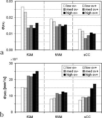
The standard deviation of MD and FA because of motion, for all six sampling schemes. For each sampling scheme, the results are given for three ROIs. The mean values within the ROIs were as follows: FA = 0.2, 0.4, 0.8 and MD = 1100 × 10⁻⁶, 820 × 10⁻⁶, 870 × 10⁻⁶ mm²/s for the frontal GM, frontal WM, and sCC, respectively. The low sampling schemes display the largest uncertainty for FA. For MD, the opposite effect can be observed.

Motion also causes a bias in FA, which depends on the sampling scheme used. Figure 14 shows the averaged values of FA within the frontal GM, the region where the effect is most pronounced, for all six sampling schemes. Although the medium and high unit‐sphere schemes do not exhibit a strong change in FA because of motion, the low sampling schemes (and to a less extent for the medium and high overplus schemes) show a clear positive bias when motion is induced.

Figure 14.

The effect of motion on the mean estimates of FA. The light gray bars are the mean values of FA within the fGM calculated from the original non motion induced data set. The dark gray bars are the mean FA values averaged from the 1,000 motion‐induced data sets with the error bars denoting the standard deviation. The positive bias because of motion is most pronounced for the low sampling schemes.

DISCUSSION

In this study, the contributions of image noise and motion effects to the total uncertainty of MD and FA at 3 T were assessed. To improve the reliability of the DTI indices, the reproducibility of six commercially available gradient sampling schemes was determined. Additionally, the effect of motion correction was investigated. Simulations showed that both the propagation of image noise and motion effects depend on the choice of gradient sampling scheme.

Contribution of Noise and Motion

Noise simulations showed that the precision (standard deviation) because of thermal noise lies between 15 and 40 × 10⁻⁶ mm²/s for MD and 0.02 and 0.04 for FA. Simulated motion, similar to the amount of motion in cooperative volunteers, showed a precision of 10–25 × 10⁻⁶ mm²/s for MD and 0.01–0.03 for FA. These results agree well with the test–retest variability (SD_ws) found by our in vivo analysis (SD_ws is 20–45 × 10⁻⁶ mm²/s for MD and 0.01–0.06 for FA). The accuracy (bias) of FA found in our simulations was also consistent with our experimental data. For the low sampling schemes in the fGM, for which the bias is most profound, the bias in FA because of noise is ∼0.02. The bias found by the motion simulations was 0.09. This is also in close agreement with our experimental data, which show a bias in FA of ∼0.07 when motion correction is omitted. Our results therefore show that the contribution of noise to the signal uncertainty is of the same order of magnitude as motion. Note that the results shown here are for healthy volunteers. For uncooperative patients, motion effects are expected to outweigh the contribution of noise as the precision of MD and FA increases linearly with the amount of induced motion (see Fig. 12).

Noise Effects

The performed noise simulations show that the bias of MD and FA is dependent on the level of anisotropy (Fig. 10a,c). The FA is an index parameter, which ranges from 0 to 1. At low anisotropy levels, all three eigenvalues are approximately equal. Any deviation because of errors in the DW‐signals, therefore, results in an increase in FA, causing the FA to be positively biased in the low anisotropy regime. In regions of high anisotropy, the FA is negatively biased. Noise in the data may cause the diffusion tensor to be nonpositive definite, leading to negative eigenvalues. The effect of (nonphysical) negative eigenvalues can be corrected for in various ways. Here, the tensors were diagonalized after which the negative eigenvalues were set to zero, and thus restricting the FA to values ≤1. This restriction results in a skewed distribution of the high FA values causing the negative bias (see Fig. 15a). This bias may be reduced by using more refined tensor estimation methods [Hasan and Narayana, 2003; Koay et al., 2006; Landman et al., 2008].

Figure 15.

The distribution of FA values at three levels of anisotropy (0.1, 0.5, and 0.9) (a) and the signal intensities of both the DW signal (b = 800) and the non‐DW signal (b = 0) from which the ADC is calculated (b). In (a), the histograms of all samples (500 orientations × 5,000 repetitions) obtained from the noise simulations are plotted for three levels of anisotropy. For both FA = 0.1 and FA = 0.9, the distributions are clearly skewed, as the FA is restricted to values between 0 and 1. Figure (b) shows the theoretical noise distributions of signal intensities at b = 0 and b = 800. For the non‐DW signal, the noise is Gaussian distributed. For the DW signal, the noise distribution is skewed, resulting in an overestimation of the DW signal and therefore underestimation of the ADC. The gray line illustrates the logarithmic fit from which the ADC would have been estimated if the noise displayed a Gaussian distribution.

The MD is prone to a negative bias at all levels of anisotropy and is progressively underestimated as FA increases. The underestimation of MD can be attributed to the Rician distribution of the noise in magnitude MR images with low SNR [Edelstein et al., 1984; Kingsley, 2006]. As seen in Figure 15b, the noise on the DW signal no longer displays a Gaussian distribution for low signal intensities. For this reason, signal intensities in DW images are positively biased when high diffusivities are measured. Because the high SNR b ₀‐image remains unaffected, the resulting ADC will be underestimated. The underestimation is most severe for anisotropic media, because the diffusivities measured along the principle axis (i.e., the long axis of the ellipsoid) are much higher than the diffusivities measured in the other directions and therefore most prone to underestimation. In the isotropic case, only moderate diffusivities are measured in each direction, which are less prone to underestimation.

Our simulations show that increasing the directional resolution is more beneficial than increasing NSA for the bias and rotational variance (for both MD and FA) and the experimental variance of FA. This is in agreement with previous studies [Jones, 2004; Jones et al., 1999; Papadakis et al., 1999, 2000; Skare et al., 2000b]. Note that, the rotational variance (i.e., the error bars in Fig. 10a,c) is only a small portion of the experimental variance. Only at the highest levels of anisotropy, the rotational variance has a noticeable contribution to the total variance for the overplus schemes. The experimental variance displays a different dependency on directional resolution and gradient strength for MD and FA. For MD, the unit‐sphere schemes exhibit a considerably larger experimental variance than the overplus schemes, which increases as the directional resolution is increased. The differences in experimental variance are smaller for FA, but appear to decrease as the directional resolution is increased. The experimental variance of MD, however, did not comply with the general perception that increasing the directional resolution is preferable to increasing the number of signal averages. In fact, the opposite effect was observed. This suggests that for FA, which reflects the amount of directionality, a dense sampling of the 3D space is required. MD, on the other hand, benefits more from a high SNR of the DW‐images; either because of shorter echo times (overplus sampling schemes) or more signal averages (low directional resolution).

According to Skare et al. [2000a], the noise performance of a sampling scheme depends on the condition number of the transformation matrix. However, the performances of the investigated sampling schemes were not quite in line with the expected noise propagation based on the condition numbers (Table I). The overplus sampling schemes, investigated in this study, have better performance than expected based on their condition numbers. In practice, when echo time and the number of collected images are not necessarily matched, parameters such as image SNR and number of signal averages may outweigh the effect of the condition number. Hence, the effects of the gradient amplitude (i.e., overplus versus unit sphere sampling schemes) appeared to be negligible.

Motion Effects

Although at 3 T the noise effects are reduced because of the higher SNR, our in vivo results showed that the effect of the sampling schemes is comparable to what has been reported for 1.5 T. Similar to what Ni et al. [2006] have reported, we found that sampling schemes with only six directions showed deviant results for FA from schemes with 15 and 32 directions. The reason for this is that the propagation of motion effects is also influenced by the choice of sampling scheme. The motion simulations show that the low sampling schemes affect the outcome of the DTI experiments distinctively different from the other sampling schemes investigated in this study. For MD, the low schemes are favorable over the medium and the high sampling schemes in terms of precision. For FA, however, the low schemes display poor precision. The medium and high (overplus and unit‐sphere) schemes exhibit a more comparable performance.

The in vivo experiments show similar results to the motion simulations. When the data are not corrected for motion, the low sampling schemes display a considerably lower precision than when motion correction is performed (see Fig. 5). The medium and high sampling schemes displayed similar reproducibility. Therefore, in terms of the ability to discriminate normal from abnormal tissue, the sampling schemes are comparable. This is applicable to both voxel‐based as ROI‐based studies, as both methods gave similar results (see Fig. 8). Moreover, the low sampling schemes are prone to a positive bias, most pronounced in isotropic regions such as the fGM. This effect has also been reported by others [Landman et al., 2007]. Landman et al. hypothesize that the bias found for sampling schemes with low directional resolution (Ndir = 6) may be caused by the nontensor behavior (e.g., crossing fibers), present in approximately one‐third of the brain voxels [Behrens et al., 2007]. However, the results from our motion simulations (see Fig. 14) suggest that the overestimation of FA by sampling schemes with low directional resolution may be caused by motion effects. This explanation is supported by our in vivo data. Additionally, the poorer sampling characteristics of sampling schemes with a low directional resolution are more likely to result in an overestimation of FA values. In the case, where the magnitude of all axes is similar (hence low FA), a poor sampling will easily end up in a detected big difference of the main axis (always resulting in increased FA values). The overestimation of FA for the low sampling schemes and the fact that the overestimation decreases when motion correction is performed supports the notion that the main cause for the positive bias of FA is the effect of motion.

Motion Correction

Motion causes the precision of DTI data and the derived MD and FA maps to be spatially dependent. Because of motion, the test–retest variability (given by SD_ws) increases strongly near the interfaces of different brain structures. Motion correction reduces the SD_ws by realigning the voxels with similar tissue content for all DW‐images. As expected, the decrease of SD_ws was most pronounced at the edges of the brain, where small amounts of motion can cause large signal variations. Our results further show that motion correction improves the reproducibility of DTI quantities. The largest increase was obtained for the low sampling schemes. For the medium‐ and high sampling schemes, only a subtle increase was obtained (see Fig. 5). Note that the in vivo experiments are performed on cooperative, relatively young, healthy subjects. Patient data, on the other hand, might be more strongly affected by motion and motion correction might have a greater impact.

Eddy Currents

Strong gradients employed in DW imaging cause eddy current distortions in the acquired EPI images. Eddy currents can be significantly reduced by a variety of methods such as self‐shielded gradient coils [Roemer and Hickey, 1993], rearrangement of the diffusion sensitive gradients [Reese et al., 2003], or gradient compensation [Glover and Pelc, 1987]. They can however not be entirely eliminated [Rohde et al., 2004]. To address the effects of the remaining eddy currents, one can choose to perform retrospective eddy current correction based on field‐maps [Jezzard et al., 1998]. In this study, however, special effort was made to reduce the potential distortions caused by the residual eddy currents by shortening the echo train as much as possible. As a result, no eddy current‐induced distortions were noticeable on visual inspection of the data. It was therefore decided not to address the effect of retrospective eddy current correction in this study.

Regional Versus Voxel‐Based Studies

There has been increasing interest in using DW MR imaging in clinical studies to localize cerebral abnormalities because of development, degeneration, or various pathologies. For the last years, an increasing number of studies are being published in which patient groups are investigated with the aid of DTI [Concha et al., 2006; Dengler et al., 2005; Kuhl et al., 2005; Nave et al., 2007; Righini et al., 1994; Sage et al., 2007]. The two main approaches used for the quantitative analysis of DTI data are as follows: ROI‐based and voxel‐based analysis. In this study, we found that the reproducibility of both methods is comparable. Recently, Snook et al. [2007] reported that the voxel‐based method and ROI‐based method gave comparable results for widespread reductions of MD and FA. However, discrepancies between the two methods (i.e., missing regions) were also found, and were attributed to problems related to the spatial normalization. Spatial normalization enables the comparison of several tissue characteristics from different subjects on a voxel‐based level. However, the normalization procedure itself encompasses several steps that might be unfavorable for the outcomes of the assessment of reproducibility characteristics of the different sampling schemes. Visual inspection of the normalized FA images revealed that the borders of distinctive structures (e.g., putamen, CC) do not always align perfectly. This might explain the large error bars obtained for the sCC (Fig. 7b). For small structures as the sCC, any misalignment (between the subjects or between sessions) will have a large effect on the within‐subject or between‐subject variability. In general, for any multisubject study, care should be exercised when performing voxel‐based analysis on small well‐defined white matter structures. Ideally, one would like to be able to differentiate the effect of sampling scheme or motion from the normalization procedure. It might be worthwhile to use more dedicated software such as Tract‐Based Spatial Statistics [Smith et al., 2006], to assure better alignment of the fibers.

Limitations

Although our simulations give good insight in the effects of motion on the accuracy of MD and FA, it is a simplification of the reality. The motion simulation used here has a few shortcomings. First, the simulated motion trajectories were created by defining a random walk with equal step size. In practice, however, motion may be more erratically (e.g., head‐twitches). Second, in vivo images were used for the simulation analyses, which inherently contain noise. The calculated uncertainties in DTI indices are therefore not only determined by motion, but may also be affected by intrinsic image noise. However, the use of in vivo‐based simulations was necessary to assess the regional differences in the brain and compare those with the in vivo experiments. Although the estimated contribution of motion is thus less accurate than that of image noise, we feel that the performed motion simulations suffice to estimate the order of magnitude of the error induced by motion for the different gradient sampling schemes.

The reproducibility from both the in vivo measurements and the motion simulations yielded differences between the fGM, the fWM, and the sCC. Although these ROIs were defined based on the anatomical locations of these regions within the brain, the obtained differences in reproducibility may not necessarily be purely because of the difference in location. Two possible confounders may cause the difference: First, the total volume of the employed mask to select the regions was not identical for all ROIs. Most notably, the mask for the sCC was only 6–8% of the size of fGM and fWM. Second, the homogeneity of fiber orientations is inherently different among the ROIs. Although in the sCC the fibers are well aligned, the fWM is likely to contain multiple fiber orientations that may confound the reproducibility measure. The reason for this can be attributed to the natural between‐subject variability in the relative amounts of the different fiber populations. In general, this “extra” between‐subject variability in FA will bias the ICC index, which can be seen in Figure 7b. For these reasons, this article is not intended to function as a comparison of the reproducibility between the different regions. The three regions merely functioned as clinically representative regions with varying anisotropy to investigate the performance of sampling schemes and motion correction.

CONCLUSIONS

Both image noise and head motion have a considerable effect on the error of the DTI parameters MD and FA. The contributions of both noise and motion are found to be of the same order. Neither motion nor image noise can therefore be neglected, and should therefore be considered when interpreting DTI results. The choice of gradient sampling scheme not only affects the propagation of image noise but also the signal errors caused by motion. Nevertheless, of the six clinically available gradient schemes tested here, the gradient sampling schemes with medium‐ and high angular resolution show similar reproducibility. The sampling schemes with a low angular resolution, however, demonstrate a poor reproducibility and are prone to a positive bias for FA in isotropic media. Motion correction considerably improves the performance of these low sampling schemes by increasing the reproducibility and reducing the positive bias.

Supporting information

Additional Supporting Information may be found in the online version of this article.

Supporting Table: The gradient sampling schemes as available on a Philips Achieva 3T scanner.

REFERENCES

- Arfanakis K,Hermann BP,Rogers BP,Carew JD,Seidenberg M,Meyerand ME ( 2002): Diffusion tensor MRI in temporal lobe epilepsy. Magn Reson Imaging 20: 511–519. [DOI] [PubMed] [Google Scholar]
- Basser PJ,Pierpaoli C ( 1996): Microstructural and physiological features of tissues elucidated by quantitative‐diffusion‐tensor MRI. J Magn Reson B 111: 209–219. [DOI] [PubMed] [Google Scholar]
- Batchelor PG,Atkinson D,Hill DL,Calamante F,Connelly A ( 2003): Anisotropic noise propagation in diffusion tensor MRI sampling schemes. Magn Reson Med 49: 1143–1151. [DOI] [PubMed] [Google Scholar]
- Behrens TE,Berg HJ,Jbabdi S,Rushworth MF,Woolrich MW ( 2007): Probabilistic diffusion tractography with multiple fibre orientations: What can we gain? Neuroimage 34: 144–155. [DOI] [PMC free article] [PubMed] [Google Scholar]
- Bland JM,Altman DG ( 1986): Statistical methods for assessing agreement between two methods of clinical measurement. Lancet 1: 307–310. [PubMed] [Google Scholar]
- Bland JM,Altman DG ( 1996): Measurement error. BMJ 313: 744. [DOI] [PMC free article] [PubMed] [Google Scholar]
- Chen B,Guo H,Song AW ( 2006): Correction for direction‐dependent distortions in diffusion tensor imaging using matched magnetic field maps. Neuroimage 30: 121–129. [DOI] [PubMed] [Google Scholar]
- Concha L,Gross DW,Wheatley BM,Beaulieu C ( 2006): Diffusion tensor imaging of time‐dependent axonal and myelin degradation after corpus callosotomy in epilepsy patients. Neuroimage 32: 1090–1099. [DOI] [PubMed] [Google Scholar]
- Cramér H ( 1970): Random Variables and Probability Distributions, 3rd ed. Cambridge: Cambridge University Press. [Google Scholar]
- Davison AC,Hinkley DV ( 1997): Bootstrap Methods and Their Application. Cambridge: Cambridge University Press. [Google Scholar]
- Dengler R,von Neuhoff N,Bufler J,Krampfl K,Peschel T,Grosskreutz J ( 2005): Amyotrophic lateral sclerosis: New developments in diagnostic markers. Neurodegener Dis 2: 177–184. [DOI] [PubMed] [Google Scholar]
- Edelstein WA,Bottomley PA,Pfeifer LM ( 1984): A signal‐to‐noise calibration procedure for NMR imaging systems. Med Phys 11: 180–185. [DOI] [PubMed] [Google Scholar]
- Farrell JA,Landman BA,Jones CK,Smith SA,Prince JL,van Zijl PC,Mori S ( 2007): Effects of signal‐to‐noise ratio on the accuracy and reproducibility of diffusion tensor imaging‐derived fractional anisotropy, mean diffusivity, and principal eigenvector measurements at 1.5 T. J Magn Reson Imaging 26: 756–767. [DOI] [PMC free article] [PubMed] [Google Scholar]
- Ge Y,Law M,Grossman RI ( 2005): Applications of diffusion tensor MR imaging in multiple sclerosis. Ann N Y Acad Sci 1064: 202–219. [DOI] [PubMed] [Google Scholar]
- Glover GH,Pelc NJ ( 1987): A method for magnetic field gradient eddy current compensation. US Patent 4698591.
- Hasan KM,Narayana PA ( 2003): Computation of the fractional anisotropy and mean diffusivity maps without tensor decoding and diagonalization: Theoretical analysis and validation. Magn Reson Med 50: 589–598. [DOI] [PubMed] [Google Scholar]
- Hasan KM,Parker DL,Alexander AL ( 2001): Comparison of gradient encoding schemes for diffusion‐tensor MRI. J Magn Reson Imaging 13: 769–780. [DOI] [PubMed] [Google Scholar]
- Henkelman RM ( 1985): Measurement of signal intensities in the presence of noise in MR images. Med Phys 12: 232–233. [DOI] [PubMed] [Google Scholar]
- Horsfield M,Lai M,Webb S,Barker G,Tofts P,Turner R,Rudge P,Miller D ( 1996): Apparent diffusion coefficients in benign and secondary progressive multiple sclerosis by nuclear magnetic resonance. Magn Reson Med 36: 393–400. [DOI] [PubMed] [Google Scholar]
- Jansen JFA,Kooi ME,Kessels AGH,Nicolay K,Backes WH ( 2007): Reproducilbility of quantitative cerebral T2 relaxometry, diffusion tensor imaging, and 1H magnetic resonance spectroscopy at 3.0 Tesla. Invest Radiol 42: 327–337. [DOI] [PubMed] [Google Scholar]
- Jenkinson M,Bannister P,Brady M,Smith S ( 2002): Improved optimization for the robust and accurate linear registration and motion correction of brain images. Neuroimage 17: 825–841. [DOI] [PubMed] [Google Scholar]
- Jezzard P,Barnett AS,Pierpaoli C ( 1998): Characterization of and correction for eddy current artifacts in echo planar diffusion imaging. Magn Reson Med 39: 801–812. [DOI] [PubMed] [Google Scholar]
- Jones DK ( 2004): The effect of gradient sampling schemes on measures derived from diffusion tensor MRI: A Monte Carlo study. Magn Reson Med 51: 807–815. [DOI] [PubMed] [Google Scholar]
- Jones DK,Basser PJ ( 2004): Squashing peanuts and smashing pumpkins: How noise distorts diffusion‐weighted MR data. Magn Reson Med 52: 979–993. [DOI] [PubMed] [Google Scholar]
- Jones DK,Horsfield MA,Simmons A ( 1999): Optimal strategies for measuring diffusion in anisotropic systems by magnetic resonance imaging. Magn Reson Med 42: 515–525. [PubMed] [Google Scholar]
- Kingsley PB ( 2006): Introduction to diffusion tensor imaging mathematics: Part III. Tensor calculation, noise, simulations, and optimization. Concepts Magn Reson Part A 28A: 155–179. [Google Scholar]
- Koay CG,Chang LC,Carew JD,Pierpaoli C,Basser PJ ( 2006): A unifying theoretical and algorithmic framework for least squares methods of estimation in diffusion tensor imaging. JMagn Reson 182: 115–125. [DOI] [PubMed] [Google Scholar]
- Kuhl CK,Textor J,Gieseke J,von Falkenhausen M,Gernert S,Urbach H,Schild HH ( 2005): Acute and subacute ischemic stroke at high‐field‐strength (3.0‐T) diffusion‐weighted MR imaging: Intraindividual comparative study. Radiology 234: 509–516. [DOI] [PubMed] [Google Scholar]
- Landman BA,Farrell JA,Jones CK,Smith SA,Prince JL,Mori S ( 2007): Effects of diffusion weighting schemes on the reproducibility of DTI‐derived fractional anisotropy, mean diffusivity, and principal eigenvector measurements at 1.5T. Neuroimage 36: 1123–1138. [DOI] [PMC free article] [PubMed] [Google Scholar]
- Landman BA,Farrell JA,Huang H,Prince JL,Mori S ( 2008): Diffusion tensor imaging at low SNR: Nonmonotonic behaviors of tensor contrasts. Magn Reson Imaging 26: 790–800. [DOI] [PMC free article] [PubMed] [Google Scholar]
- Le Bihan D,Mangin JF,Poupon C,Clark CA,Pappata S,Molko N,Chabriat H ( 2001): Diffusion tensor imaging: Concepts and applications. J Magn Reson Imaging 13: 534–546. [DOI] [PubMed] [Google Scholar]
- Marenco S,Rawlings R,Rohde GK,Barnett AS,Honea RA,Pierpaoli C,Weinberger DR ( 2006): Regional distribution of measurement error in diffusion tensor imaging. Psychiatry Res 147: 69–78. [DOI] [PMC free article] [PubMed] [Google Scholar]
- Nave RD,Foresti S,Pratesi A,Ginestroni A,Inzitari M,Salvadori E,Giannelli M,Diciotti S,Inzitari D,Mascalchi M ( 2007): Whole‐brain histogram and voxel‐based analyses of diffusion tensor imaging in patients with leukoaraiosis: Correlation with motor and cognitive impairment. AJNR Am J Neuroradiol 28: 1313–1319. [DOI] [PMC free article] [PubMed] [Google Scholar]
- Ni H,Kavcic V,Zhu T,Ekholm S,Zhong J ( 2006): Effects of number of diffusion gradient directions on derived diffusion tensor imaging indices in human brain. AJNR Am J Neuroradiol 27: 1776–1781. [PMC free article] [PubMed] [Google Scholar]
- Papadakis NG,Xing D,Huang CL,Hall LD,Carpenter TA ( 1999): A comparative study of acquisition schemes for diffusion tensor imaging using MRI. J Magn Reson 137: 67–82. [DOI] [PubMed] [Google Scholar]
- Papadakis NG,Murrills CD,Hall LD,Huang CL,Adrian Carpenter T ( 2000): Minimal gradient encoding for robust estimation of diffusion anisotropy. Magn Reson Imaging 18: 671–679. [DOI] [PubMed] [Google Scholar]
- Papanikolaou N,Karampekios S,Papadaki E,Malamas M,Maris T,Gourtsoyiannis N ( 2006): Fractional anisotropy and mean diffusivity measurements on normal human brain: Comparison between low‐and high‐resolution diffusion tensor imaging sequences. Eur Radiol 16: 187–192. [DOI] [PubMed] [Google Scholar]
- Pierpaoli C,Jezzard P,Basser PJ,Barnett A,Di Chiro G ( 1996): Diffusion tensor MR imaging of the human brain. Radiology 201: 637–648. [DOI] [PubMed] [Google Scholar]
- Reese TG,Heid O,Weisskoff RM,Wedeen VJ ( 2003): Reduction of eddy‐current‐induced distortion in diffusion MRI using a twice‐refocused spin echo. Magn Reson Med 49: 177–182. [DOI] [PubMed] [Google Scholar]
- Righini A,Pierpaoli C,Alger J,Di Chiro G ( 1994): Brain parenchyma apparent diffusion coefficient alterations associated with experimental complex partial status epilepticus. Magn Reson Med 12: 865–871. [DOI] [PubMed] [Google Scholar]
- Roemer PB,Hickey JS ( 1993): Self‐shielded gradient coils for nuclear magnetic resonance imaging. US patent 4737716.
- Rohde GK,Barnett AS,Basser PJ,Marenco S,Pierpaoli C ( 2004): Comprehensive approach for correction of motion and distortion in diffusion‐weighted MRI. Magn Reson Med 51: 103–114. [DOI] [PubMed] [Google Scholar]
- Sage CA,Peeters RR,Gorner A,Robberecht W,Sunaert S ( 2007): Quantitative diffusion tensor imaging in amyotrophic lateral sclerosis. Neuroimage 34: 486–499. [DOI] [PubMed] [Google Scholar]
- Schaefer PW,Copen WA,Lev MH,Gonzalez RG ( 2006): Diffusion‐weighted imaging in acute stroke. Magn Reson Imaging Clin N Am 14: 141–168. [DOI] [PubMed] [Google Scholar]
- Skare S,Hedehus M,Moseley ME,Li T‐Q ( 2000a): Condition number as a measure of noise performance of diffusion tensor data acquisition schemes with MRI. J Magn Reson 147: 340–352. [DOI] [PubMed] [Google Scholar]
- Skare S,Li T,Nordell B,Ingvar M ( 2000b): Noise considerations in the determination of diffusion tensor anisotropy. Magn Reson Imaging 18: 659–669. [DOI] [PubMed] [Google Scholar]
- Smith SM, Jenkinson M, Johansen‐Berg H, Rueckert D, Nichols TE, Mackay CE, Watkins KE, Ciccarelli O, Cader MZ, Matthews PM and Behrens TEJ. ( 2006): Tract‐based spatial statistics: Voxelwise analysis of multi‐subject diffusion data. Neuroimage 31: 1487–1505. [DOI] [PubMed] [Google Scholar]
- Snook L,Plewes C,Beaulieu C ( 2007): Voxel based versus region of interest analysis in diffusion tensor imaging of neurodevelopment. Neuroimage 34: 243–252. [DOI] [PubMed] [Google Scholar]
- Tofts P ( 2003): Quantitative MRI of the Brain Measuring Changes Caused by Disease. Hoboken, NJ: Wiley. [Google Scholar]
- Toosy AT,Ciccarelli O,Parker GJ,Wheeler‐Kingshott CA,Miller DH,Thompson AJ ( 2004): Characterizing function‐structure relationships in the human visual system with functional MRI and diffusion tensor imaging. Neuroimage 21: 1452–1463. [DOI] [PubMed] [Google Scholar]
- Wang C, Stebbins GT, Nyenhuis DL, deToledo‐Morrell L, Freels S, Gencheva E, Pedelty L, Sripathirathan K, Moseley ME, Turner DA, Gabrieli JDE, Gorelick PB. ( 2006): Longitudinal changes in white matter following ischemic stroke: A three‐year follow‐up study. Neurobiol Aging 27: 1827–1833. [DOI] [PubMed] [Google Scholar]
- Zhu T,Liu X,Connelly PR,Zhong J ( 2008): An optimized wild bootstrap method for evaluation of measurement uncertainties of DTI‐derived parameters in human brain. Neuroimage 40: 1144–1156. [DOI] [PubMed] [Google Scholar]
Associated Data
This section collects any data citations, data availability statements, or supplementary materials included in this article.
Supplementary Materials