

Abstract
Functional magnetic resonance imaging (fMRI) has become an important tool in Neuroscience due to its noninvasive and high spatial resolution properties compared to other methods like PET or EEG. Characterization of the neural connectivity has been the aim of several cognitive researches, as the interactions among cortical areas lie at the heart of many brain dysfunctions and mental disorders. Several methods like correlation analysis, structural equation modeling, and dynamic causal models have been proposed to quantify connectivity strength. An important concept related to connectivity modeling is Granger causality, which is one of the most popular definitions for the measure of directional dependence between time series. In this article, we propose the application of the partial directed coherence (PDC) for the connectivity analysis of multisubject fMRI data using multivariate bootstrap. PDC is a frequency domain counterpart of Granger causality and has become a very prominent tool in EEG studies. The achieved frequency decomposition of connectivity is useful in separating interactions from neural modules from those originating in scanner noise, breath, and heart beating. Real fMRI dataset of six subjects executing a language processing protocol was used for the analysis of connectivity. Hum Brain Mapp, 2009. © 2007 Wiley‐Liss, Inc.
Keywords: fMRI, connectivity, Granger causality, frequency domain, multisubject, bootstrap
INTRODUCTION
Functional magnetic resonance imaging (fMRI) has become one of the most prominent techniques in Neuroscience. It was first introduced by Ogawa [1990], who studied the properties of BOLD signal (blood oxygenation level dependent), based on paramagnetic properties of deoxyhemoglobin (T2* weighted acquisition). Because of its noninvasive and high spatial resolution properties, the number of studies based on fMRI has been growing considerably.
The main focus of most fMRI studies is the localization of neural activation, for which identification and modeling methods are well established [Frackowiak et al., 1997]. Actually, most of them rely on general linear model (GLM), measuring the association of observed BOLD signal and an expected haemodynamic response function (HRF). By contrast, connectivity modeling and identification remain open questions. Several studies [Biswal et al. 1995; Cordes et al. 2000; Peltier and Noll, 2001] are based on BOLD correlation analysis (BCA), which can be interpreted as a measure of concurrence between the signals of two brain areas. Despite being useful as an exploratory tool, BCA is unsuited for connectivity characterization because it is based solely on the bivariate analysis of relationships and the identified connections are undirected, i.e., BCA neither provides information about the multivariate influences among time series nor about the direction of information flow.
Advanced statistical approaches have been proposed to overcome these weaknesses. The most popular techniques to address connectivity in fMRI are: the structural equation modeling (SEM), proposed for fMRI data analysis by McIntosh [1998] and dynamic causal models (DCM), introduced by Friston et al. [2003]. However, both techniques rely on a priori specification of the connectivity linkages, i.e., the structural graph must be previously known. These approaches are suited to test the statistical significance of the covariance structure between neural areas with known effective connectivity. For this reason, they cannot be considered exploratory tools, but rather just confirmatory methods for some hypothesis.
Recently, Granger causality identification using vector autoregressive (VAR) models has been a useful tool for understanding cortical interactions. Granger [1969] defined causality in terms of predictability and temporal precedence. This concept was first applied in econometrics to identify temporal relationships among financial time series. Granger causality identification using VAR methods can be considered both an exploratory and also a modeling tool. In contrast to SEM and DCM, VAR modeling does not require any pre‐specification or a priori knowledge about the connectivity structure, even though a priori information can also be included in the model as constraints in the parametric space. Furthermore, considering some graph theoretical ideas, Eichler [2005] introduced connectivity identification based on Granger causality and graphical modelling. Goebel et al. [2003], Roebroeck et al. [2005] and Abler et al. [2006] introduced the Granger causality mapping in the context of fMRI experiments. They also showed the reproducibility and reliability of the connectivity identification via Granger causality for BOLD signals. Valdes‐Sosa et al. [2005] applied VAR models to fMRI datasets considering estimation in cases of overparametrization and sparse models using penalized regression. Considering the case of nonstationary signals, Sato et al. [2006a, 2006b] introduced intervention VAR and time varying VAR models to infer the connectivity in fMRI datasets.
Frequency domain multivariate modelling is also the aim of interest of many researchers, as Parseval's relationship allows decomposing signal variance into its frequency components. BOLD signal variance is composed of unobserved haemodynamic response, scanner noise, heart beating, habituation effect, and other factors. Sun et al. [2004] suggested the use of spectral coherence and partial coherence to attain frequency domain connectivity identification in fMRI and illustrated their application in motor experiments. Salvador et al. [2005] introduced an approach based on partial coherence named normalized partial mutual information, and have shown that functional connectivity lay mainly in low frequencies (0.0004, 0.1518 Hz). In spite of being a useful exploratory tool, like BCA, spectral coherence does not allow inferring directionality in the connectivity structure.
In this article, we employ partial directed coherence (PDC) to identify neuronal connectivity using fMRI data. This approach does not require structural pre‐specification and is very well defined in multivariate cases. The viability and usefulness of this method is illustrated through a language‐processing paradigm.
METHODS
Granger Causality
Granger [1969] defined the concept of causality by focusing on the description of temporal relationships between time series. The bases of the Granger causality concept are the reduction in prediction error and the fact that the effect cannot precede its cause. For two scalar time series x t and y t, there is Granger causality from series x t to y t if the past values of x t increase the forecast power of present and value of y t. It formalizes the notion of amount of information flow from the area of the signal x t to the area of y t. It is important to remark that the Granger causality relationship is not reciprocal, that is, existence of Granger causality from x t to y t does not imply the existence of Granger causality from y t to x t and vice‐versa. Furthermore, Granger causality does not imply physical and biological causality, but only predictability improvement (functional connectivity).
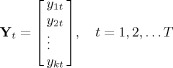
VAR modeling is the most common approach used for Granger causality identification. Let Y t a multidimensional time series composed by k signals, i.e.
 |
(1) |
where by the VAR model is defined as
| (2) |
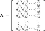
and v is a vector of constants and ε t is a vector of random disturbances. The matrices A l (l = 1,…,p) are given by
 |
(3) |
and the element
 is the causality coefficient from the series y
jt to the series y
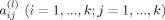
it. The vector of innovations ϵ
t has a covariance matrix given by
is the causality coefficient from the series y
jt to the series y
it. The vector of innovations ϵ
t has a covariance matrix given by
 |
(4) |
Note that assuming the expectation of ε t to be zero, the prediction of Y t given all the information available until the time (t − 1) is given by
| (5) |
Hence, considering the VAR model, y
jt is said to Granger‐cause y
it if the coefficient
 is non zero for some value of l. This can be interpreted as existence of information flow from the brain area j to brain area i. In practice, inferences about the connectivity structure can be achieved by fitting a VAR model to the observed BOLD signal and by testing the statistical significance of the “causality” coefficients. Further description, discussion and estimation algorithms can be found in Lütkepohl [1993].
Partial Directed Coherence
Although conceptually interesting, in its original form Granger causality is a time domain concept, and does not permit discerning the frequency domain characteristics of the signals involved and which play important roles in data interpretation. For instance, artifacts or non‐neuronal physiological signals like cardiac and respiratory signals can be distinguished using their frequency characteristics. This is an important advantage over common time domain analysis where these non‐neuronal signals have to be eliminated somehow most often by ad hoc methods, when that comes to be done at all.
Whereas defining Granger causality is straightforward in the case of pairs of time series, multivariate generalizations are less obvious [Geweke, 1984; Hosoya, 2001]. To overcome these difficulties, partial directed coherence (PDC) was introduced [Sameshima and Baccalá, 1999; Baccalá and Sameshima, 2001], developed [Schelter et al., 2006; Baccalá and Sameshima, 2001] and a considerable amount of successful applications in neurophysiology have been done [Fanselow et al., 2001; Yang et al., 2005; Supp et al., 2005; Schlogl and Supp, 2006].
A useful form of PDC called generalized PDC (GPDC) is achieved by suitable normalization [Baccalá et al., 2006, Baccalá et al., 2007] so that frequency domain causality from the j‐th time series to the i‐th time series at frequency λ is defined as:
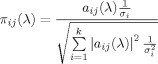 |
(6) |
where
| (7) |
for δ ij = 1 if i = j and 0 otherwise. It is clear that null GPDC in all frequencies indicates absence of Granger causality and vice versa.
The main advantage of GPDC remains in its interpretability as a measure of strength of connectivity between neural structures. The square modulus of GPDC value from j‐th time series by i‐th series can be understood intuitively as the proportion of the power spectra of the j‐th time series, which is sent to the i‐th series considering the effects of the other series. Furthermore, it can be shown to be a factor in the decomposition of the coherence in the bivariate case and of partial coherence in the multivariate case. Hence, zero GPDC (π ij(λ) = 0) can be interpreted as absence of functional connectivity from the j‐th structure to the i‐th structure at frequency λ and high GPDC, near one, indicates strong connectivity between the structures.
In the literature there are also other measures of neural connectivity in the frequency domain. For instance, directed transfer function (DTF) and relative power contribution (RPC) have been used for the analysis of EEG [Kaminski et al., 2001] and fMRI [Yamashita et al., 2005], respectively. However, in the bivariate case, GPDC, DTF, and RPC are all equivalent in the sense that when one of them is zero the others are also zero. The difference becomes evident in the multivariate case when PDC is the frequency domain counterpart of Granger causality in time domain [Lütkepohl, 1993; Baccalá and Sameshima, 2001]. Actually, DTF and RPC are not able to distinguish between direct and indirect pathways linking different structures; thus they do not provide the multivariate relationships from a partial perspective.
To provide a common comparative picture PDC's properties are contrasted to those of other connectivity methods in Table I.
Table I.
Comparison between connectivity models
| Frequency specification | Intensity interpretation | Directionality | Partial relationship | |
|---|---|---|---|---|
| Pearson correlation | No | Yes | No | No |
| Granger causality test | No | No | Yes | Yes |
| Coherence | Yes | Yes | No | No |
| Partial coherence | Yes | Yes | No | Yes |
| PDC | Yes | Yes | Yes | Yes |
| DTF | Yes | Yes | Yes | No |
| RPC | Yes | Yes | Yes | No |
Multisubject Hypothesis Testing Using Bootstrap
Most fMRI studies are based on multiple subject analysis for inference about the population. Because of its robustness against outliers (which are common in medical studies), the median GPDC coefficient across subjects is an attractive group statistic. However, the distribution of the median GPDC's across subjects under the null hypothesis of zero GPDC in specific frequencies is difficult to obtain mainly because magnetic resonance noise is non‐Gaussian [Wink and Roerdink, 2006] and the number of subjects in fMRI experiments is usually small. In this case, results about asymptotic distribution of quantiles are not adequate. Thus, we suggest the following bootstrap algorithm to obtain the statistical significance of the group GPDC statistic:
Step 1: Fit VAR models for the BOLD time series of each subject separately.
Step 2: Obtain the VAR coefficient estimates and residuals for each subject.
Step 3: For each frequency, calculate the GPDC estimates [see Eq. (7)].
Step 4: Obtain the median GPDC across subjects at each frequency (observed GPDC).
Step 5: For each subject, resample the residuals (random sampling with replacement) obtained in Step 2.
Step 6: To test each influence from time series j to i, assume a model where the VAR coefficients a , l = 1,…,p (i.e., all coefficients related to time series j causing i) are 0. The other VAR coefficients remain as originally estimated by least squares in Step 2. Basically, this step consists of assuming a model under the assumption of no Granger causality from time series j to i, and thus can be used to generate bootstrap samples under the null hypothesis.
Step 7: By using the resampled residuals obtained in Step 5, and the model specified in Step 6, simulate a bootstrap multivariate time series (note that this procedure generates time series under the null hypothesis of no “causality” from time series j to i).
Step 8: Obtain the median GPDC for this bootstrap sample.
Step 9: Go to step 5 until the desired number of bootstrap samples is achieved.
Step 10: Estimate the critical value for each frequency using the respective median GPDC bootstrap samples. The critical value is defined as the (1 − α) quantile of bootstrap samples, where α is the expected Type I Error.
Step 11: Compare the observed median GPDC with the estimated critical value.
A diagram of the previous steps is presented in Figure 1. This is a general algorithm that may be applied to any statistic obtained by using any function of GPDC coefficients. This is a useful property, as any hypothesis on moments or quantiles can be tested analogously and independently on the distribution of the data.
Figure 1.
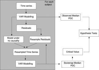
Diagram of bootstrap GPDC testing.
Data Acquisition and Experiment
In this study, six healthy subjects executed a language‐related task. Incomplete sentences with a missing word were visually (text) presented to them. The missing word was reveled only after a short time interval, allowing the subjects to process the sentence. Illustrative examples of this task are the sentences: “He posted the letter without a …” or “The leaves are already falling from the …”. The stems were presented for 2,500 ms, followed by a blank screen. After an interval of 700 ms the target word appeared (e.g., “stamp”). The subjects were asked to respond if the target word adequately complete or not the sentence by using a yes/no button box. After the response, an asterisk replaced the target word until the beginning of the next trial.
Eighty sentences were presented to the subjects (in five runs of 16 trials) in fixed intervals of 20.4 s, corresponding to 12 time points per sentence. In other words, the subjects were asked to complete different sentences periodically in a cycle of 12 points. The aim of this experiment was to identify the areas activated when subjects did these tasks to study sentence processing in healthy controls.
Gradient echo‐planar images were acquired in a 1.5 Tesla magnetic resonance GE system (General Electric, Milwaukee, WS) at the Maudsley Hospital, Institute of Psychiatry, King's College London. The total number of volumes was 960, acquired using T2* weighted MR images depicting BOLD contrast (parallel to intercomissural plane, TE = 40 ms, TR = 1.7 s, in plane resolution = 3.125 mm, thickness = 7.0 mm, gap = 0.7 mm, flip angle = 90°) [Arcuri et al., 2000].
Images Processing
The fMRI data was preprocessed by using head motion realignment (rigid body transformation), slice time correction, spatial smoothing (Gaussian kernel with size of five voxels) and normalization to the space of Talairach and Tournoux [1988]. The group activation maps were obtained using the GLM assuming an HRF function composed of two Poisson functions with peeks in 9.1 (activation) and 13.1 s (undershoot) after the presentation of sentences. The events modeled by GLM refer mainly to the time when the target word appears and there is a cognitive processing about the adequacy of the presented sentence and this word, corrected by the haemodynamic delay. These steps were carried out using the fMRI XBAM software [Brammer et al., 1997], freely available at http://www.brainmap.co.uk).
RESULTS AND DISCUSSION
Figure 2 shows the brain activation maps. Significant activations (cluster wise P‐values <0.01) were found in cerebellum (Tal: 7, −78, −24), primary visual cortex (V1; Tal: 0, −85, 9), left superior temporal gyrus (STG; Tal: −51, 4, −2), left Insula (Tal: −47, 4, 9) and Thalamus (Tal: 11, −8, 0).
Figure 2.
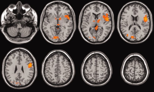
Language task activation maps (cluster wise P‐value <0.01). [Color figure can be viewed in the online issue, which is available at www.interscience.wiley.com.]
The primary visual cortex, superior temporal gyrus and Insula were selected as regions of interest (ROI) for the connectivity analysis. The information flow characterization between these three areas was then assessed using GPDC. Because of low frequency artifacts, which lead to nonstationarity characteristics to the signals, the difference operator was applied to ROI's average time series. The series were then normalized to zero mean and unit variance. Figures 3 and 4 illustrate the ROI's time series for one subject and the average periodogram across subjects, respectively.
Figure 3.
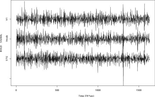
Illustrative ROIs' time series of a subject.
Figure 4.
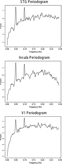
ROIs' average periodogram across subjects.
Language understanding and sentences processing are extremely complex processes. First, the auditory (or visual) stimuli must be translated into meaningful subjective concepts, the underlying message must be understood, and argumentation must be processed.
BA‐17 is a sensory cortical area located in the calcarine sulcus (occipital lobe) and corresponds to the primary visual cortex (or striate cortex). In this experiment, incomplete sentences were presented visually, and thus, visual cortex activation was expected. Broadman area 22 (BA‐22) in the lateral aspect of the superior temporal gyrus is classically involved in processing auditory signals and language reception being a major component of Wernicke's area, the main neuronal module in language comprehension. Hence, sentence comprehension involves activity in this area. Further, BA‐72 in Insula is involved in language understanding and processing. In this experiment, subjects were asked to decide if the target word complete the sentences presented, implying that the paradigm involves not only language understanding but also the analysis of semantic meaning.
It is important to highlight that these three areas do not work independently, but form an integrated network. Sonty et al. [2007] studied the changes in the effective connectivity of language networks in cases of primary progressive aphasia. Obleser et al. [2007] have shown that function integration of brain regions improves speech perception. Karunanayaka et al. [2007] identified that language connectivity structure when children listen to histories is age‐related.
Note that the ROI's periodograms in Figure 4 show significant power at 0.049 Hz (and 0.098 Hz, a harmonic), which is exactly the stimulation frequency in this paradigm. This result is expected as the ROI's were identified as regions which respond to the stimulus. In addition, harmonic peaks are expected, since the haemodynamic response differs significantly from sinusoidal functions. Using multisubject GPDC analysis (Figs. 5 and 7), we found evidence of a connectivity network involving the ROIs' concentrated mostly at 0.049 and 0.098 Hz. A diagram representing the connectivity graph obtained using the median PDC only at 0.049 Hz is shown in Figure 6. The relationship between these areas directly related to the execution of the task is expected to occur at this frequency. Panel STG to Insula (see Fig. 5) shows that there are significant energies at other frequencies (e.g., frequencies less than 0.03, at 0.07 Hz or 0.13 Hz), indicating the existence of relationships between these areas, as mirrored by the BOLD time series, but which are unrelated to processing the task. Low frequency acquisition artifacts are frequent in long scanning fMRI sessions. PDC is useful to discriminate between stimulus‐induced functional connectivity from other sources. However, the physiological origin (cardiac, breath, etc.) of the connectivity generated by these other sources may be difficult to discriminate, since aliasing is present in the data and oscillatory components of BOLD signal and artifacts are still not completely identified or established. Thus, additional care must be to taken when designing the experiment, because aliasing problems may overlap the stimulation frequency.
Figure 5.
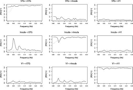
ROIs' multisubject median partial directed coherence. The dotted line shows the 95% confidence upper bound under the hypothesis of no connectivity between the nodes.
Figure 7.
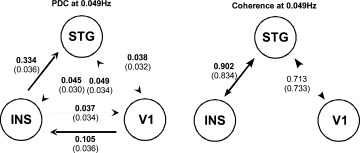
Multisubject median partial directed coherence at 0.049Hz, simple coherence at 0.049Hz (using the same bootstrap algorithm). The frequency of stimulation in the language paradigm was 0.049Hz. The thick solid lines describe the links with relevant intensity of information flow. The critical regions at 5% of significance are values greater than the shown in parentheses.
Figure 6.
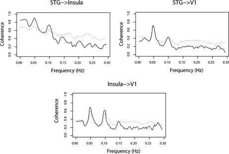
ROIs' multisubject median coherence function. The dotted line shows the 95% confidence upper bound under the hypothesis of no connectivity between the nodes (critical region).
Figure 7 indicates strong information flow from the Insula to STG, where ∼33% of the spectrum energy of Insula at 0.049 Hz (see Fig. 5) is sent to STG. Furthermore, PDC analysis shows significant amount of information from the visual cortex (11% of the energy) to the Insula, which is reasonable, as the sentences were presented visually. The other connections are marginally significant (near statistical threshold) and show low power (less than 5%), indicating no relevant information flow. In summary, multisubject GPDC analysis suggests that participants read the sentences; the information migrates from the primary visual cortex to the Insula and then to STG. Figures 6 and 7 show the estimated coherence function between the ROI areas which show patterns similar to GPDC, but is unable to pinpoint link directionality hindering its interpretation (see Table I).
The statistical power of VAR model‐based connectivity estimators like PDC is a compromise between the number of ROIs, number of lags considered, and signal duration. Lags increase the parameters that need to be estimated in a linear fashion, whereas the number of considered ROIs does so quadratically. Hence including regions that do not significantly participate in the connectivity network implies a sharp decrease in the power to identify links. One may try to circumvent this problem by constraining the number of parameters in the model, i.e., by specifying the linkages a priori, even though this limits the PDC's usefulness as an exploratory tool. In fMRI experiments, our experience with typical signal durations, suggests selecting a maximum of five or six areas for inclusion in the analysis.
A second limitation involving fMRI experiments with the execution of multiple tasks is that they do not provide information about what is being processed nor where each cognitive component of the task is processed and much less how this information is processed to produce behavior. In the present case, GPDC may help infer the interactions between the areas activated in the task, suggesting the existence of connectivity networks, with a periodic information flow at the frequency of stimulation, besides being able to pinpoint the direction of this flow. Note, however that the inferred information pathway is not enough to assess whether semantic interpretation or sentence completion happen at the Insula, the STG or both. The answer to this question is conceivably only possible by comparing the present results to other studies, as one cannot draw such conclusions from the present data/experimental paradigm alone.
In view of these limitations, future works will require elaborating paradigms and sequences of stimulation to separate the cognitive components, using state “subtractions” or similar techniques [Amaro and Barker, 2006]. However, the discrimination between task‐related and other components provided by GPDC represents a starting point in addressing these questions.
CONCLUSION
In this article, we introduced a method for connectivity inference between neural structures which: (1) is based on Granger causality concept, (2) is able to discriminate physiological and nonphysiological components based on their frequency characteristics, (3) is multivariate, i.e., it considers the partial/direct relationships between all pairs of time series. Also a bootstrap procedure for the median normalized GPDC analysis of fMRI data is proposed.
Acknowledgements
The fMRI experiment was part of SMA's PhD studies supervised and partially supported by Prof. Philip K. McGuire, to whom we are grateful.
REFERENCES
- Abler B,Roebroeck A,Goebel R,Hose A,Schonfeldt‐Lecuona C,Hole G,Walter H( 2006): Investigating directed influences between activated brain areas in a motor‐response task using fMRI. Magn Reson Imaging 24: 181–185. [DOI] [PubMed] [Google Scholar]
- Amaro E Jr,Barker GJ( 2006): Study design in fMRI: Basic principles. Brain Cogn 60: 220–232. Review. [DOI] [PubMed] [Google Scholar]
- Arcuri SM,Amaro E Jr,Kircher TT,Andrew C,Brammer M,Willians SSC,Giampietro V,McGuire PK ( 2000): Neural correlates of the semantic processing of sentences: effects of Cloze probability in an event‐related fMRI study. Neuroimage 5: S333. [Google Scholar]
- Baccalá LA,Sameshima K( 2001): Partial directed coherence: A new concept in neural structure determination. Biol Cybern 84: 463–474. [DOI] [PubMed] [Google Scholar]
- Baccalá LA,Takahashi YD,Sameshima K( 2006): Computer intensive testing for the influence between time series In Handbook of Time Series Analysis. Berlin: Wiley VCH; pp 365–388. [Google Scholar]
- Baccalá LA,Takahashi DY,Sameshima K( 2007): Generalized Partial Directed Coherence. Proceedings of the 2007,15th International Conference on Digital Signal Processing(DSP2007). IEEE 1: 162–166.
- Brammer MJ,Bullmore ET,Simmons A,Williams SC,Grasby PM,Howard RJ,Woodruff PW,Rabe‐Hesketh S( 1997): Generic brain activation mapping in functional magnetic resonance imaging: A nonparametric approach. Magn Reson Imaging 15: 763–770. [DOI] [PubMed] [Google Scholar]
- Biswal B,Yetkin FZ,Haughton VM,Hyde JS( 1995): Functional connectivity in the motor cortex of resting human brain using echo‐planar MRI. Magn Reson Med 34: 537–541. [DOI] [PubMed] [Google Scholar]
- Cordes D,Haughton VM,Arfanakis K,Wendt GJ,Turski PA,Moritz CH,Quigley MA,Meyerand ME( 2000): Mapping functionally related regions of brain with functional connectivity MR imaging. AJNR Am J Neuroradiol 21: 1636–1644. [PMC free article] [PubMed] [Google Scholar]
- Eichler M( 2005): A graphical approach for evaluating effective connectivity in neural systems. Philos Trans R Soc Lond B Biol Sci, 360: 953–967. [DOI] [PMC free article] [PubMed] [Google Scholar]
- Fanselow EE,Sameshima K,Baccala LA,Nicolelis MA( 2001): Thalamic bursting in rats during different awake behavioral states. Proc Natl Acad Sci USA, 98: 15330–15335. [DOI] [PMC free article] [PubMed] [Google Scholar]
- Frackowiak RSJ,Friston KJ,Frith CD,Dolan RJ,Mazziotta JC( 1997): Human Brain Function. CA: Academic Press. [Google Scholar]
- Friston KJ,Harrison L,Penny W( 2003): Dynamic causal modelling. Neuroimage 19: 1273–1302. [DOI] [PubMed] [Google Scholar]
- Goebel R,Roebroeck A,Kim DS,Formisano E( 2003): Investigating directed cortical interactions in time‐resolved fMRI data using VAR modeling and Granger causality mapping. Magn Reson Imaging 21: 1251–1261. [DOI] [PubMed] [Google Scholar]
- Geweke J( 1984): Measurement of conditional linear dependence and feedback between time series. Journal of the American Statistical Association 79: 907–915. [Google Scholar]
- Granger CWJ( 1969): Investigating causal relations by econometric models and cross‐spectral methods. Econometrica 37: 424–438. [Google Scholar]
- Hosoya Y( 2001): Elimination of third‐series effect and defining partial measures of causality. J Time Series Anal 22: 537–554. [Google Scholar]
- Kaminski M,Ding M,Truccolo WA,Bressler SL( 2001): Evaluating causal relations in neural systems: Granger causality, directed transfer function and statistical assessment of significance. Biol Cybern 85: 145–157. [DOI] [PubMed] [Google Scholar]
- Karunanayaka PR,Holland SK,Schmithorst VJ,Solodkin A,Chen EE,Szaflarski JP,Plante E( 2007): Age‐related connectivity changes in fMRI data from children listening to stories. Neuroimage 34: 349–360. [DOI] [PubMed] [Google Scholar]
- Lütkepohl H( 1993): Introduction to Multiple Time Series Analysis. New York: Springer‐Verlag. [Google Scholar]
- McIntosh AR( 1998): Understanding neural interactions in learning and memory using functional neuroimaging. Ann NY Acad Sci 8: 556–571. [DOI] [PubMed] [Google Scholar]
- Obleser J,Wise RJ,Alex Dresner M,Scott SK( 2007): Functional integration across brain regions improves speech perception under adverse listening conditions. J Neurosci 27: 2283–2289. [DOI] [PMC free article] [PubMed] [Google Scholar]
- Ogawa S,Lee TM,Kay AR,Tank DW( 1990): Brain magnetic resonance imaging with contrast dependent on blood oxygenation. Proc Natl Acad Sci USA 87: 9868–9872. [DOI] [PMC free article] [PubMed] [Google Scholar]
- Peltier SJ,Noll DC( 2001): T2* Dependence of low frequency functional connectivity. Neuroimage 16: 985–992. [DOI] [PubMed] [Google Scholar]
- Roebroeck A,Formisano E,Goebel R( 2005): Mapping directed influence over the brain using Granger causality and fMRI. Neuroimage 25: 230–242. [DOI] [PubMed] [Google Scholar]
- Salvador R,Suckling J,Schwarzbauer C,Bullmore E( 2005): Undirected graphs of frequency dependent functional connectivity in whole brain networks. Phil Trans R Soc B 360: 937–946. [DOI] [PMC free article] [PubMed] [Google Scholar]
- Sameshima K,Baccala LA( 1999): Using partial directed coherence to describe neuronal ensemble interactions. J Neurosci Methods 94: 93–103. [DOI] [PubMed] [Google Scholar]
- Sato JR,Amaro E Jr,Takahashi DY,Felix MM,Brammer MJ,Morettin PA( 2006a): A method to produce evolving functional connectivity maps during the course of an fMRI experiment using wavelet‐based time‐varying Granger causality. Neuroimage 31: 187–196. [DOI] [PubMed] [Google Scholar]
- Sato JR,Takahashi DY,Cardoso EF,Morais‐Martin MG,Amaro E Jr,Morettin PA( 2006b): Intervention models in functional connectivity identification applied to fMRI. Int J Biomed Imaging 1: 1–7. [DOI] [PMC free article] [PubMed] [Google Scholar]
- Schelter B,Winterhalder M,Eichler M,Peifer M,Hellwig B,Guschlbauer B,Lucking CH,Dahlhaus R,Timmer J( 2006): Testing for directed influences among neural signals using partial directed coherence. J Neurosci Methods 152: 210–219. [DOI] [PubMed] [Google Scholar]
- Schlogl A,Supp G( 2006): Analyzing event‐related EEG data with multivariate autoregressive parameters. Prog Brain Res 159: 135–147. Review. [DOI] [PubMed] [Google Scholar]
- Sonty SP,Mesulam MM,Weintraub S,Johnson NA,Parrish TB,Gitelman DR( 2007): Altered effective connectivity within the language network in primary progressive aphasia. J Neurosci 27: 1334–1345. [DOI] [PMC free article] [PubMed] [Google Scholar]
- Sun FT,Miller LM,D'Esposito M( 2004): Measuring interregional functional connectivity using coherence and partial coherence analyses of fMRI data. Neuroimage 21: 647–658. [DOI] [PubMed] [Google Scholar]
- Supp GG,Schlogl A,Gunter TC,Bernard M,Pfurtscheller G,Petsche H( 2004): Lexical memory search during N400: Cortical couplings in auditory comprehension. Neuroreport 15: 1209–1213. [DOI] [PubMed] [Google Scholar]
- Talairach J,Tournoux P( 1988): Co‐Planar Stereotaxic Atlas of the Human Brain. New York: Thieme. [Google Scholar]
- Valdes‐Sosa PA,Sanchez‐Bornot JM,Lage‐Castellanos A,Vega‐Hernandez M,Bosch‐Bayard J,Melie‐Garcia L,Canales‐Rodriguez E( 2005): Estimating brain functional connectivity with sparse multivariate autoregression. Philos Trans R Soc Lond B Biol Sci 360: 969–981. [DOI] [PMC free article] [PubMed] [Google Scholar]
- Yamashita O,Sadato N,Okada T,Ozaki T( 2005): Evaluating frequency‐wise directed connectivity of BOLD signals applying relative power contribution with the linear multivariate time‐series models. Neuroimage 25: 478–490. [DOI] [PubMed] [Google Scholar]
- Yang H,Chang JY,Woodward DJ,Baccala LA,Han JS,Luo F( 2005): Coding of peripheral electrical stimulation frequency in thalamocortical pathways. Exp Neurol 196: 138–152. [DOI] [PubMed] [Google Scholar]
- Wink AM,Roerdink JBTM( 2006): BOLD noise assumptions in fMRI. Int J Biomed Imaging 1: 1–11. [DOI] [PMC free article] [PubMed] [Google Scholar]