

Abstract
Independent component analysis (ICA) of functional MRI data is sensitive to model order selection. There is a lack of knowledge about the effect of increasing model order on independent components' (ICs) characteristics of resting state networks (RSNs). Probabilistic group ICA (group PICA) of 55 healthy control subjects resting state data was repeated 100 times using ICASSO repeatability software and after clustering of components, centrotype components were used for further analysis. Visual signal sources (VSS), default mode network (DMN), primary somatosensory (S1), secondary somatosensory (S2), primary motor cortex (M1), striatum, and precuneus (preC) components were chosen as components of interest to be evaluated by varying group probabilistic independent component analysis (PICA) model order between 10 and 200. At model order 10, DMN and VSS components fuse several functionally separate sources that at higher model orders branch into multiple components. Both volume and mean z‐score of components of interest showed significant (P < 0.05) changes as a function of model order. In conclusion, model order has a significant effect on ICs characteristics. Our findings suggest that using model orders ≤20 provides a general picture of large scale brain networks. However, detection of some components (i.e., S1, S2, and striatum) requires higher model order estimation. Model orders 30–40 showed spatial overlapping of some IC sources. Model orders 70 ± 10 offer a more detailed evaluation of RSNs in a group PICA setting. Model orders > 100 showed a decrease in ICA repeatability, but added no significance to either volume or mean z‐score results. Hum Brain Mapp, 2010. © 2010 Wiley‐Liss, Inc.
Keywords: FMRI, ICA, model order, PICA, resting‐state networks
INTRODUCTION
Recently, independent component analysis (ICA) as a blind source separation technique has become a major data‐driven analysis tool for functional MRI (fMRI) studies [Biswal and Ulmer, 1999, Calhoun et al., 2001, Kiviniemi et al., 2003; McKeown et al., 1998]. It has been successfully applied for separating statistically independent blood oxygen level dependent (BOLD) components associated with both task‐related and spontaneous resting state activity within neuronal networks [Beckmann et al., 2005; Bell and Sejnowski, 1995; Greicius et al., 2004; Kiviniemi et al., 2000; McKeown et al., 1998; Van de Ven et al., 2004]. An essential advantage of ICA over hypothesis‐driven techniques is that the former allows for differentiating relevant functional brain signals from various sources of noise without a priori knowledge on the signal origin [Biswal and Ulmer,, 1999; Calhoun et al., 2003; Hyvärinen et al., 2001; McKeown et al., 1998, 2003]. And at present it is an open question on how many of the ongoing functions simultaneously occurring in the brain (in rest or task state) can be detected with BOLD technique.
Based on statistical features of the data such as the profile of joint density distributions, ICA separates components from BOLD data into a number of spatially or temporally independent components (ICs) [Biswal and Ulmer, 1999; Calhoun et al., 2001; McKeown et al., 1998]. Non‐Gaussianity of joint density distributions are maximized with a projection pursuit methodology [Hyvärinen and Oja, 2000]. ICA algorithms begin the projection pursuit with a guess and produce components in a random order. The number of calculated ICA components, that is, model order, can be freely selected from 1 to n − 1, where n is the number of imaged brain volumes (spatial ICA), or number of voxels in the volume of interest (temporal ICA).
Investigators have raised a question regarding what the right amount of calculated ICA components are. Studies focused on both resting state and activation suggested that functionally connected regions would be split into separate components when the data dimensionality is overestimated [Moritz et al., 2005; Van de Ven et al., 2004]. On the other hand, when too few components are calculated, ICA was said to mix various components [Bartels and Zeki, 2005; Esposito et al., 2003; McKeown et al., 1998; Van de Ven et al., 2004]. An excessive reduction of the dimensionality may be particularly problematic for analysis of resting state fluctuations, since some of the sources of interest may have a weak signal compared to noise. Our group has recently shown that a 42 signal sources can be robustly depicted from the brain using high model order group probabilistic independent component analysis (PICA) [Kiviniemi et al., 2009].
Recently, two groups have estimated an appropriate number of ICA components for fMRI data. Ma et al. [2007] investigated the influence of the number of ICs on the ability of spatial ICA to capture resting state functional connectivity, showing that results of ICA could be affected by the number of ICs if this number is too small. However, only volume of functional sources detected within a range of 2–30 ICA components was evaluated. Li et al. [2007] proposed a subsampling scheme to obtain a set of independent and identically distributed data samples from the dependent data samples using the information‐theoretic criteria for order selection. The method was applied on the simulated data and data from a visuomotor task showing that when ICA is performed at overestimated orders, the stability of the IC estimates decreases and the estimation of task‐related brain activations show degradation.
The aim of this study was to investigate the role of model order on group PICA of resting state data. In this study we investigate the effect of increasing dimensionality on spatial features, repeatability, and emergence of resting state signal sources. It was hypothesized that the above characteristics of ICA components are significantly affected by model order increase. Visual signal sources (VSS), default mode network (DMN), primary somatosensory (S1), secondary somatosensory (S2), primary motor cortex (M1), striatum, and precuneus (preC) components were chosen as components of interest to be evaluated from resting state data.
MATERIALS AND METHODS
Subjects
The ethical committee of Oulu University Hospital has approved the studies for which the subjects have been recruited, and informed consent has been obtained from each subject individually according to the Helsinki declaration. Fifty‐five control subjects were chosen (age 24.96 ± 5.25 years, 32 ♀, 23 ♂) from three resting state studies: an At Risk Mental Stage 1986 birth cohort study of ADHD and schizophrenia; a 1966 birth cohort study of schizophrenia; brain tumor resting state study, total n = 200.
Imaging Methods
Subjects were imaged on a GE 1.5T HDX scanner equipped with an 8‐channel head coil using parallel imaging with an acceleration factor 2. The scanning was done during January 2007 to May 2008. All subjects received identical instructions: to simply rest and focus on a cross on an fMRI dedicated screen that they saw through the mirror system of the head coil. Hearing was protected using ear plugs, and motion was minimized using soft pads fitted over the ears.
The functional scanning was performed using an EPI GRE sequence. The TR used was 1,800 ms and the TE was 40 ms. The whole brain was covered, using 28 oblique axial slices 4‐mm thick with a 0.4‐mm space between the slices. FOV was 25.6 cm × 25.6 cm with a 64 × 64 matrix, and a flip angle of 90°. The resting state scan consisted of 253 functional volumes. The first three images were excluded due to T1 equilibrium effects. In all three studies, the resting state scanning started the protocols, and lasted 7 min and 36 s. In addition to resting‐state fMRI, T1‐weighted scans were taken with 3D FSPGR BRAVO sequence (FOV 24.0 cm, matrix 256 × 256, slice thickness 1.0 mm, TR 12.1 ms, TE 5.2 ms, and flip angle 20°) in order to obtain anatomical images for coregistration of the fMRI data to standard space coordinates.
Data Preprocessing
Head motion in the fMRI data was corrected using multiresolution rigid body coregistration of volumes, as implemented in FSL 3.3 MCFLIRT software [Jenkinson et al., 2002]. The default settings used were: middle volume as reference, a three‐stage search (8 mm rough + 4 mm, initialized with 8 mm results + 4 mm fine grain, initialized with the previous 4 mm step results) with final tri‐linear interpolation of voxel values, and normalized spatial correlation as the optimization cost function. Brain extraction was carried out for motion‐corrected BOLD volumes with optimization of the deforming smooth surface model, as implemented in FSL 3.3 BET software [Smith, 2002] using threshold parameters f = 0.5 and g = 0; and for 3D FSPGR volumes, using parameters f = 0.25 and g = 0. After brain extraction, the BOLD volumes were spatially smoothed; 7 mm FWHM Gaussian kernel and voxel time series were detrended using a Gaussian linear high‐pass filter with a 125‐s cutoff. The FSL 4.0 fslmaths tool was used for these steps.
Multiresolution affine coregistration as implemented in the FSL 4.0 FLIRT software [Jenkinson et al., 2002] was used to coregister mean nonsmoothed fMRI volumes to 3D FSPGR volumes of corresponding subjects, and 3D FSPGR volumes to the Montreal Neurological Institute (MNI) standard structural space template (MNI152_T1_2mm_brain template included in FSL). Tri‐linear interpolation was used, a correlation ratio was used as the optimization cost function, and regarding the rotation parameters a search was done in the full [‐π π] range. The resulting transformations and the tri‐linear interpolation were used to spatially standardize smoothed and filtered BOLD volumes to the 2‐mm MNI standard space. Because an sICA was run later on fMRI data concatenated from the 55 subjects, in practice the spatial resolution of spatially standardized BOLD volumes had to be lowered to 4 mm.
ICA Analysis
ICA analysis was carried out using FSL 4.0 MELODIC software implementing PICA [Beckmann and Smith, 2004] framework and ICASSO [Himberg et al., 2004] in MATLAB (The Math Work, Natick, MA). Temporal concatenation option in MELODIC was used to perform PICA‐related preprocessing and data conditioning in group analysis setting. PCA‐reduced datasets from MELODIC were produced for model orders of 10, 20, 30, 40, 50, 60, 70, 80, 90, 100, 125, 150, and 200. These data were analyzed using ICASSO repeating FastICA [Hyvärinen, 1999] 100 times with strict convergence threshold (1 × 10⁻⁷) using skewness as the contrast function.
The mixing matrix containing cluster centrotype‐based estimates from ICASSO was used to produce final IC maps. These maps were converted to z‐score maps by dividing intensity values by voxelwise estimates of noise standard deviation provided by original MELODIC output files. All z‐score maps were thresholded using mixture modeling (P = 0.5) in MELODIC.
VSS, DMN, S1, S2, M1, striatum, and preC were chosen as components of interest to be evaluated from resting state data. ICA characteristics including volume, mean z‐score, and its standard deviation were calculated using fslstats tool included with FSL4. Statistical analyses of components' volume and mean z‐score as a linear function of ICA model order were performed using Origin software (OriginPro 8 SR0, V8.0725 “B725”) and statistical parameters of significance were set at a level (P < 0.05).
We observed detection points and branching points for each of the signal source of interest. Detection point refers to the lowest model order in which the signal source was initially detected and branching point means the model order where a selected signal source splits into two components. Cluster quality index (I q) of the selected components from ICASSO‐runs [Himberg et al., 2004] were used to assess the repeatability of ICA components of interest and mean of all I q was used to measure the overall stability of the whole ICA decomposition. Mean I q threshold (Repeatability threshold) was chosen to be ≥0.8.
The Juelich histological atlas [Eickhoff et al., 2007], and the Harvard‐Oxford cortical and subcortical atlases (Harvard Center for Morphometric Analysis) that are provided with the FSL4 software were used to quantify anatomical characteristics of thresholded z‐score maps. Identification and detection of ICA components was accomplished by visual selection using fslview software. An FSL4 fslstats tool was used to calculate the number of nonzero voxels in selected thresholded components (DMNA, DMNP, VSSL, VSSM, VSS1, VSS2, VSS3, preC, and M1), which was divided by the number of nonzero voxels of the anatomical templates included in the used anatomical atlases, to provide a percentage of coverage of different anatomical areas by each IC.
RESULTS
Spatial Stability
Components of interest such as, DMN, VSS, and preC were represented in ICA components throughout all calculated model orders. However, at the lowest estimated model order (model order 10) only one representative DMN, VSS, and preC component could be identified. At higher model orders, both DMN and VSS components branched into multiple components without being affected by un‐related voxel clusters, essentially covering the initial low model order component completely. On the other hand, preC did not show any branching after it was first detected. At model order 20, DMN branched mainly into anterior (DMNA) and posterior (DMNP) sources, while VSS component branched into medial (VSSM) and lateral (VSSL). VSS further branched into subcomponents (VSS1, VSS2, and VSS3) at model orders 30, 50 and 70, respectively (see Fig. 1).
Figure 1.
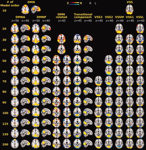
Example images showing the effect of increasing model order on resting state DMN, DMN‐related and VSS components. At model order 10, components such as DMN and VSS were detected then at model order 20 both DMN and VSS branched into [DMNA and DMNP] and VSS into [VSSL and VSSM]. Then at model order 30, VSS1, DMN‐related and the transitional component emerged. At model order 50, VSS2 component emerged, DMN‐related branched into two subcomponents. A transitional zone where a spatial overlapping and transition of activated brain regions took place (model orders 30–40). At model order 70, VSS3 component emerged.
M1 emerged at model order 20, showing no clear splitting at higher model orders. At model order 30, two components of interest (S1, S2) emerged and neither of them branched at higher model orders (see Fig. 2). In addition to that, two other components were detected (see Fig. 1). First component is overlapping with DMN parietal regions. This DMN‐related component branched at higher model orders into two separate components focused on middle temporal gyrus, angular gyrus, and inferior frontal gyrus in either left or right dominantly. The second is a transitional component (involving bilateral occipital cortices, lingual gyrus, and lower part of precuneus), which represents overlapping between various signal sources. The transition among these sources is most visible at 30–40 model orders. At model order 40, striatum and M2 components emerged and later branched into right and left dominant subcomponents at model orders 100 and 60, respectively (see Fig. 2).
Figure 2.
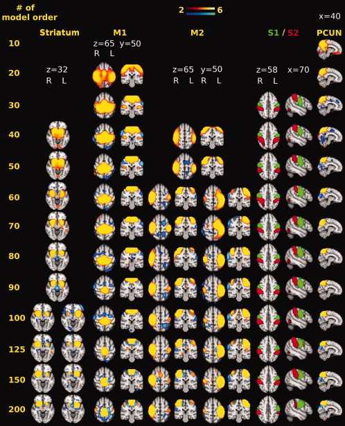
Example images showing the effect of increasing model order on resting state striatum, M1, M2, S1, S2, and preC components. S1 and S2 are shown in green and red for visual feasibility purposes. At model order 10, preC emerged. M1 appeared at model order 20. Both S1 and S2 emerged at model order 30 showing no branching at higher model orders. Then at model order 40, both M2 and striatum components were detected and then later branched into right or left dominant components at model orders 60 and 100, respectively.
Anatomical coverage results of the ICs concerning the brain regions defined in anatomical atlases were performed on selected model orders (20, 30, 70, and 200). Results showed that the coverage of different anatomical structures by selected ICs was decreasing as a function of model order and also the number of atlas templates covered by an IC was decreasing as a function of model order (Results are not shown).
We have identified low spatial frequency components in the white matter characterized by a presence of rounded patches with a high z‐score center and a low z‐score periphery. These white matter components emerged at model order 40 and increased in number as a function of model order.
Volume and z‐Score
Both volume and mean z‐score showed significant changes as a result of increasing the ICA model order. Volume of all components of interest except DMNP (P = 0.06) decreased significantly (P < 0.05) as a function of model order. Almost all components of interest showed a significant linear decrease (P < 0.05) in volume reaching model orders 70–80 (see Fig. 3). On the other hand, all components of interests showed a general trend of increase as a function of model order, but only half of them showed a significant increase in mean z‐score up to model orders 70–80. Neither volume nor mean z‐score showed any improvement in significance at model orders higher than 80.
Figure 3.

On the left side, volume of all components of interest except DMNP (P = 0.06) show a significant decrease (P < 0.05) as a function of model order. All components of interest except S1 and S2 show a maximum significant decrease in volume up to model orders 70–80. Above model order 80, no significant changes in volume occur. On the right side, mean z‐score of all components of interest show a general trend of increase as a function of model order. DMNP, VSSL, S2, and preC show a significant increase in mean z‐score up to model orders 70–80. Above model order 80, no significant changes occur in mean z‐score.
Detection and Branching Points
There was variability in both detection and branching points among different signal sources. DMN, VSS, and preC were detected at model order 10. M1 emerged at model order 20 followed by S1, S2, and VSS1 at model order 30. Both M2 and striatum components emerged at model order 40. Then VSS2 and VSS3 were detected at model orders 50 and 70, respectively. Some model orders (i.e., 20 and 50) represented both detection and branching points at the same time (c.f. Figs. 1 and 2).
Repeatability of ICA Components
Repeatability of ICA decomposition was evaluated using the mean I q for each model order. Mean I q reaches its highest value at the lowest model order and then shows a significant decrease in repeatability as a function of model order (P = 2 × 10⁻⁷, c.f. Fig. 4A). We have also used the I q of each component of interests in order to evaluate ICASSO components' repeatability as a function of model order. Almost all components of interest showed a decrease in repeatability at higher model orders. DMNA, VSSL, and striatum showed varying repeatability below model order 60, followed by relative stable repeatability up to model order 100. DMNP and VSSM showed high stable repeatability below model order 50, and then their repeatability decreased gradually as a function of model order. preC showed varying repeatability between 40 and 70, then high stable repeatability between 80 and 150. Both S1 and M1 showed high stable repeatability, followed by a decrease in repeatability above model orders 100 and 150, respectively. S2 showed a varying repeatability up to model order 100, after that its repeatability decreased gradually (Fig. 4B).
Figure 4.

(A) ICASSO components' repeatability represented by mean of cluster quality index (I q) showing a significant decrease as a function of model order (P = 2 × 10⁻⁷). (B) I q of resting state DMNA, DMNP, VSSM, VSSL, preC, and S2. Both DMNA and VSSL showed low and varying repeatability at model orders below 60 then a stable high repeatability between 60 and 100 model orders. DMNP and VSSM were relatively stable until model order 50. Between model orders 40 and 70, preCshowed varying repeatability then a stable high repeatability reaching 150. Both S1 and M1 showed stable high repeatability up to model order 100 and 150, respectively, after that their repeatability also decreased. S2 showed varying repeatability below model order 100 followed by a gradual reduction in repeatability.
DISCUSSION
In this study, we explored how ICA model order affects characteristics of the detected resting state networks (RSNs). Results show that model order has a significant effect on the characteristics of ICs. Spatial features, volume, mean z‐score, and repeatability of ICA decomposition all change significantly as a function of model order. Increasing model order increased the functional neuroanatomical precision, but reduced the repeatability of the ICA decomposition.
Spatial Stability
Our results show that at low model orders signal sources tend to merge into singular components, which then split into several subcomponents at higher model orders. These findings are consistent with previous and most recent studies showing 10–12 RSNs detected from the brain cortex using resting state data with ICA model order around 20–40 [Beckmann et al., 2005; Calhoun et al., 2008; Damoiseaux et al., 2006; De Luca et al., 2006; Smith et al., 2009] and splitting of these RSNs into subnetworks at high model orders [Smith et al., 2009]. Recently, we have shown that the brain cortex can be functionally segmented into 42 resting state signal sources and increase neuroanatomical precision in a group PICA setting [Kiviniemi et al., 2009].
Increasing the model order forces ICA to separate or branch large networks into subnetworks. However, it is not a general rule, since we have also detected other components showing no branching at higher model orders (e.g., S1 and S2). There is a lack of knowledge on neurophysiological basis explaining why some components tend to branch into more fine tuned components while others stay stable. The small‐world and scale‐free dynamics of brain networks [Van den Heuvel et al., 2008] might offer an explanation; large networks at low model orders may be connected to each other with limited number of connections. At higher model order, ICA separates large networks like DMN and VSS into several subnetworks. The stable, nonbranching components (i.e., S1 and S2) do not share many similar spatiotemporal features with other components and are therefore more functionally independent. In terms of network characteristics the stable components might be less connected nodes, while branching ones are kind of connector hubs, performing a variety of tasks and receiving information from multiple nodes [Achard et al., 2006; Van den Heuvel et al., 2008]. Thus it would be interesting to investigate temporal connectivity dynamics of these components. The differential functionality of the subnetworks (e.g., DMNA and DMNP) forming the larger networks (e.g., DMN) at lower model orders may play a role in explaining why these components tend to branch at higher model orders [Buckner et al., 2009; Calhoun et al., 2008; Esposito et al., 2005, 2009; Kim et al., 2009; Mayer et al., 2009; Uddin et al., 2009].
Seifritz et al. [2002] showed spatial ICA components of both primary and secondary auditory cortices, where the time courses of these spatial ICs were characterized by an initial peak (transient component), and then a plateau (sustained component). This temporal pattern suggested the presence of two concurrent temporally independent processes. Then by temporally decomposing the signals from the spatial ICA into temporally ICs, they were able to identify transient and sustained components of human auditory cortex.
The transitional zone is a range of model orders at which overlapping and transition among signal sources occurred. Results showed a transitional zone (model orders 30–40) where inferior parts of precuneus, bilateral occipital cortices, and lingual gyrus were involved. Overlapping of various signal sources and transition among them along with model order increase does not mean that model orders involved are factitious. Instead, it is an additive proof showing the effect of increasing model order on ICs' spatial characteristics.
The negative source activations (blue color in Figs. 1 and 2) are somewhat smaller in size than the positive activations (yellow‐red color), which in our opinion talks against an artificial source of anti‐correlation. Mathematically FastICA requires centering of the data, which is close to global signal regression as a preprocessing step. However, the spatial ICA approach does not involve any temporal normalization but rather it occurs in the spatial domain. Therefore, the detected negative correlations are not a product of temporal signal regression. Also after ICA analysis, the data has been rotated freely in order to maximize non‐Gaussianity of the source distributions. It seems highly unlikely that the negative z‐scores in spatial IC maps are “artificial.” Regarding FastICA as a spatial ICA method (in fMRI data analysis) these deactivations have not been studied enough to make valid claims, and for their current interpretability, we advice caution. In this article, we tend to focus on positive z‐score maps. Therefore, we think that a separate study would be proper for such methodological considerations.
Anatomical coverage results showed that both the coverage percentage and the total number of overlapped anatomical templates by selected ICs were decreasing as a function of model order. Components at high model orders tend to focus on specific anatomical templates or split into left and right dominant subnetworks. Splitting of large networks (at higher model orders) into subnetworks might be representing a split into subfunctions [Smith et al., 2009].
Combining the findings above shows that low model orders (e.g., model order ≤20) provide a general picture of large scale brain networks but components such as S2, VSS1, and VSS3 that emerged at higher model orders might then be missed. Therefore in order not to miss such valuable components (cortical and subcortical), higher model orders should be used in group PICA settings.
ICA Algorithm Repeatability
ICASSO mean I q of each calculated model order significantly decreased as a function of model order. But with the mean I q not falling below 0.8 at model orders <100, it suggests a relatively good repeatability below model order100 (Fig. 4A). In addition, the I q for each component of interest showed a general tendency of decrease at model orders >100 even with the most spatially stable components such as S1 (Fig. 4B). These findings are consistent with both mean z‐score and volume results showing no improvement in significance at model orders higher than 80.
Model Order
Importantly, we would like to note that the very low model orders in ICA of fMRI data produce a more of a general functional unit mapping technique. The detected large components at model orders 10–20 represent a guide in the detection of large functional network clusters, which share some common feature that makes them independent in a macroscopic scale. Low model order components showing large networks are more repeatable based on the I q values when compared to higher model orders. Investigation of their activity has so far produced several important findings and they lead the way into understanding how the global functionality is orchestrated in the brain.
Zhao et al. [2004] reported that ICA has some characteristics to which attention must be given. The model order used for ICA analysis is crucial for the reliability of the ICA method. If too few components are calculated, a weak functional signal source might be missed, while calculations with too many components can result in overfitting, which leads to components consisting of just a single spike at different locations [Hyvärinen, 1999; Zhao et al., 2004]. Särelä and Vigário, addressing the overlearning problem described two types of overlearning, the first kind results in the generation of spike‐like signals if there are not enough samples in the data or there is a considerable amount of noise present. The second is characterized by low frequency bumps if the data also has power spectrum characterized by a 1/f curve [Särelä and Vigario, 2003].
Volume, mean z‐score, and ICA components' repeatability were all significantly affected by model order selection. In general, low model orders showed the highest volume and I q values. Increasing model order resulted in a significant changes in both volume and mean z‐score reaching its peak around 70–80 model order. Further increase of model order showed a significant decrease in I q values, but added no significance in either volume or mean z‐score values.
Based on our findings calculation of 70 ± 10 model orders: (i) sufficiently separates signal sources, (ii) is repeatable enough (I q > 0.8), (iii) does not over‐fit the data, and (iv) showed significant changes in both volume and mean z‐score curves for the evaluation of RSN components in group PICA setting. This is consistent with the basic rule [Särelä and Vigario, 2003] concerning upper limit of model order that for robust estimation of N parameters (ICs) one needs T = 5 × N 2 samples: regarding our data we have samples from 27,539 voxels that corresponds to 74 ICs according to this basic rule.
In the light of these findings we could interpret our results as follows: At model orders below 20, individual signal sources tend to aggregate into singular components involving various neuroanatomically and functionally separate units that become later detectable as separate components at higher model orders. This deduction is supported by the fact that new subcomponents kept emerging at higher model orders. The use of higher model order forces the ICA to search the data for more local non‐Gaussianity maxima and therefore succeeds in separating the data into more functionally meaningful components. However as these local maxima may be subtle, repeated measures such as ICASSO offer a possibility for the depiction of these sources.
We emphasize that the 70 ± 10 component range applies to our 1.5 Tesla group PICA setting with the present imaging parameters and data preprocessings. Different model orders may be found more optimal when higher field strengths and higher resolutions are used. In addition, we have found it very fruitful to use model orders above branching points of the networks especially in the case of comparing controls to cases in certain diseases.
CONCLUSION
Increasing group PICA model order has shown a significant effect on characteristics of ICs. Spatial features, volume, mean z‐score, and ICA repeatability all change significantly as a function of model order. Both volume and mean z‐score changed significantly along with model order increase up to 70–80 model order. Increasing model order resulted in a significant reduction in ICA repeatability. Model orders ≤20 provide a general picture of large scale brain networks. However, detection of some components (i.e., S2 and striatum) required higher model orders estimation. Model orders around 30–40 showed spatial overlapping of some IC sources. Model orders 70 ± 10 offer a more detailed and yet reliable evaluation of RSN in a group PICA setting. Model orders >100 showed a decrease in ICA repeatability, but added no significance in either volume or mean z‐score values.
REFERENCES
- Achard S, Salvador R, Whitcher B, Suckling J, Bullmore E ( 2006): A resilient, low frequency, small‐world human brain functional network with highly connected association cortical hubs. J Neurosci 26: 63–72. [DOI] [PMC free article] [PubMed] [Google Scholar]
- Bartels A, Zeki S ( 2005): Brain dynamics during natural viewing conditions—A new guide for mapping connectivity in vivo. Neuroimage 24: 339–349. [DOI] [PubMed] [Google Scholar]
- Beckmann CF, Smith SM ( 2004): Probabilistic independent component analysis for functional magnetic resonance imaging. IEEE Trans Med Imaging 23: 137–152. [DOI] [PubMed] [Google Scholar]
- Beckmann CF, DeLuca M, Devlin JT, Smith SM ( 2005): Investigations into resting‐state connectivity using independent component analysis. Philos Trans R Soc Lond B Biol Sci 360: 1001–1013. [DOI] [PMC free article] [PubMed] [Google Scholar]
- Bell AJ, Sejnowski TJ ( 1995): An information‐maximization approach to blind separation and blind deconvolution. Neural Comput 7: 1004–1034. [DOI] [PubMed] [Google Scholar]
- Biswal RR, Ulmer JL ( 1999): Blind source separation of multiple signal sources on fMRI data sets using independent component analysis. J Comput Assist Tomogr 23: 265–271. [DOI] [PubMed] [Google Scholar]
- Buckner RL, Sepulcre J, Talukdar T, Krienen FM, Liu H, Hedden T, Andrews‐Hanna JR, Sperling RA, Johnson KA ( 2009): Cortical hubs revealed by intrinsic functional connectivity: Mapping, assessment of stability, and relation to Alzheimer's disease. J Neurosci 29: 1860–1873. [DOI] [PMC free article] [PubMed] [Google Scholar]
- Calhoun VD, Adali T, Pearlson GD, Pekar JJ ( 2001): Spatial and temporal independent component analysis of functional MRI data containing a pair of task‐related waveforms. Hum Brain Mapp 13: 43–53. [DOI] [PMC free article] [PubMed] [Google Scholar]
- Calhoun VD, Adali T, Hansen LK, Larsen J, Pekar JJ ( 2003): ICA of functional MRI data: An overview. Fourth International Symposium on Independent Component Analysis and Blind Signal Separation (ICA2003). 7 April, Nara, Japan; pp 281–288.
- Calhoun VD, Kiehl KA, Pearlson GD ( 2008): Modulation of temporally coherent brain networks estimated using ICA at rest and during cognitive tasks. Hum Brain Mapp 29: 828–838. [DOI] [PMC free article] [PubMed] [Google Scholar]
- Damoiseaux JS, Rombouts SA, Barkhof F, Scheltens P, Stam CJ, Smith SM, Beckmann CF ( 2006): Consistent resting‐state networks across healthy subjects. Proc Natl Acad Sci USA 104: 18760–18765. [DOI] [PMC free article] [PubMed] [Google Scholar]
- De Luca M, Beckmann CF, De Stefano N, Matthews PM, Smith SM ( 2006): fMRI resting state networks define distinct modes of long‐distance interactions in the human brain. Neuroimage 29: 1359–1367. [DOI] [PubMed] [Google Scholar]
- Eickhoff SB, Paus T, Caspers S, Grosbras MH, Evans AC, Zilles K, Amunts K ( 2007): Assignment of functional activations to probabilistic cytoarchitectonic areas revisited. Neuroimage 36: 511–521. [DOI] [PubMed] [Google Scholar]
- Esposito F, Seifritz E, Formisano E ( 2003): Real‐time independent component analysis of fMRI time‐series. Neuroimage 20: 2209–2224. [DOI] [PubMed] [Google Scholar]
- Esposito F, Scarabino T, Hyvarinen A, Himberg J, Formisano E, Comani S, Tedeschi G, Goebel R, Seifritz E, Di Salle F ( 2005): Independent component analysis of fMRI group studies by self‐organizing clustering. Neuroimage 25: 193–205. [DOI] [PubMed] [Google Scholar]
- Esposito F, Aragri A, Latorre V, Popolizio T, Scarabino T, Cirillo S, Marciano E, Tedeschi G, Di Salle F ( 2009): Does the default‐mode functional connectivity of the brain correlate with working‐memory performances? Arch Ital Biol 147: 11–20. [PubMed] [Google Scholar]
- Greicius MD, Srivastava G, Reiss AL, Menon V ( 2004): Default‐mode network activity distinguishes Alzheimer's disease from healthy aging: Evidence from functional MRI. Proc Natl Acad Sci USA 101: 4637–4642. [DOI] [PMC free article] [PubMed] [Google Scholar]
- Himberg J, Hyvärinen A, Esposito F ( 2004): Validating the independent components of neuroimaging time‐series via clustering and visualization. Neuroimage 22: 1214–1222. [DOI] [PubMed] [Google Scholar]
- Hyvärinen A ( 1999): Fast and robust fixed‐point algorithms for independent component analysis. IEEE Trans Neural Netw 10: 626–634. [DOI] [PubMed] [Google Scholar]
- Hyvärinen A, Oja E ( 2000): Independent component analysis: Algorithms and applications. Neural Netw 13: 411–430. [DOI] [PubMed] [Google Scholar]
- Hyvärinen A, Karhunen J, Oja E ( 2001): Independent Component Analysis. Wiley Interscience, New York.
- Jenkinson M, Bannister P, Brady M, Smith S ( 2002): Improved optimization for the robust and accurate linear registration and motion correction of brain images. Neuroimage 17: 825–841. [DOI] [PubMed] [Google Scholar]
- Kim Dae Il, Manoach DS, Mathalon DH, Turner JA, Mannell M, Brown GG, Ford JM, Gollub RL, White T, Wible C, Belger A, Bockholt HJ, Clarck V.P, Lauriello J, O'Leary D, Mueller BA, Lim KO, Andreasen N, Potkin SG, Calhoun VD ( 2009): Dysregulation of working memory and default‐mode networks in schizophrenia using independent component analysis, an fBRIN and MCIC study. Hum Brain Mapp 11: 3795–3811. [DOI] [PMC free article] [PubMed] [Google Scholar]
- Kiviniemi V, Jauhianen J, Paääkkö E, Vainionpää V, Oikarinen J, Rantala H, Tervonen O, Biswal BB ( 2000): Slow vasomotor fluctuation in the fMRI of the anesthetized child brain. Magn Reson Med 44: 378–383. [DOI] [PubMed] [Google Scholar]
- Kiviniemi V, Kantola J‐H, Jauhiainen J, Hyvärinen A, Tervonen O ( 2003): Independent component analysis of nondeterministic fMRI signal sources. Neuroimage 19: 253–260. [DOI] [PubMed] [Google Scholar]
- Kiviniemi V, Starck T, Jukka R, Xiangyu L, Nikkinen J, Haapea M, Veijola J, Moilanen I, Isohanni M, Zang YF, Tervonen O ( 2009): Functional segmentation of the brain cortex using high model order group PICA. Hum Brain Mapp DOI: 10.1002/hbm.20813. [DOI] [PMC free article] [PubMed] [Google Scholar]
- Li Y‐O, Adali T, Calhoun V ( 2007): Estimating the number of independent components for functional magnetic resonance imaging data. Hum Brain Mapp 11: 1251–1266. [DOI] [PMC free article] [PubMed] [Google Scholar]
- Ma L, Wang B, Chen X, Xiong J ( 2007): Detecting functional connectivity in the resting brain: A comparison between ICA and CCA. Magn Reson Imaging 25: 47–56. [DOI] [PubMed] [Google Scholar]
- Mayer JS, Roebroeck A, Maurer K, Linden DE ( 2009): Specialization in the default mode: Task‐induced brain deactivations dissociate between visual working memory and attention. Hum Brain Mapp DOI: 10.1002/hbm.20850. [DOI] [PMC free article] [PubMed] [Google Scholar]
- McKeown MJ, Makeig S, Brown GG, Kindermann S, Bell A, Sejnowski T ( 1998): Analysis of fMRI data by blind source separation into independent spatial components. Hum Brain Mapp 6: 160–188. [DOI] [PMC free article] [PubMed] [Google Scholar]
- McKeown MJ, Hansen LK, Sejnowski TJ ( 2003): Independent component analysis of functional MRI: What is signal and what is noise? Curr Opin Neurobiol 13: 620–629. [DOI] [PMC free article] [PubMed] [Google Scholar]
- Moritz CH, Carew JD, McMillan AB, Meyerand ME ( 2005): Independent component analysis applied to self‐paced functional MR imaging paradigms. Neuroimage 25: 181–192. [DOI] [PubMed] [Google Scholar]
- Särelä J, Vigário R ( 2003): Overlearning in marginal distribution‐based ICA: Analysis and solutions. J Mach Learn Res 4: 1447–1469. [Google Scholar]
- Seifritz E, Esposito F, Hennel F, Mustovic H, Neuhoff JG, Bilecen D, Tedeschi G, Scheffler K, Di Salle F ( 2002): Spatiotemporal pattern of neural processing in the human auditory cortex. Science 297: 1706–1708. [DOI] [PubMed] [Google Scholar]
- Smith SM ( 2002): Fast robust automated brain extraction. Hum Brain Mapp 17: 143–155. [DOI] [PMC free article] [PubMed] [Google Scholar]
- Smith SM, Fox PT, Miller KL, Glahn DC, Fox PM, Mackay CE, Filippini N, Watkins KE, Toro R, Laird AR, Beckmann CF ( 2009): Correspondence of the brain's functional architecture during activation and rest. Proc Natl Acad Sci USA 106: 13040–13045. [DOI] [PMC free article] [PubMed] [Google Scholar]
- Uddin LQ, Kelly AM, Biswal BB, Xavier Castellanos F, Milham MP ( 2009): Functional connectivity of default mode network components: Correlation, anticorrelation, and causality. Hum Brain Mapp 30: 625–637. [DOI] [PMC free article] [PubMed] [Google Scholar]
- Van de Ven VG, Formisano E, Prvulovic D, Roeder CH, Linden DE ( 2004): Functional connectivity as revealed by spatial independent component analysis of fMRI measurements during rest. Hum Brain Mapp 22: 165–178. [DOI] [PMC free article] [PubMed] [Google Scholar]
- Van den Heuvel MP, Stam CJ, Boersma M, Hulshoff Pol HE ( 2008): Small‐world and scale‐free organization of voxel‐based resting‐state functional connectivity in the human brain. Neuroimage 43: 528–539. [DOI] [PubMed] [Google Scholar]
- Zhao X, Glahn D, Tan LH, Li N, Xiong J, Gao J‐H ( 2004): Comparison of TCA and ICA techniques in fMRI data processing. J Magn Reson Imaging 19: 397–402. [DOI] [PubMed] [Google Scholar]