

Abstract
The superior temporal resolution of magneto‐ and electroencephalography (MEEG) provides unique insight into the dynamics of brain function. The analysis of the spatial dimensions of MEEG recordings can take a multiplicity of approaches: from the original scalp recordings to the identification of their generators through localizing or imaging techniques. Overall, both MEEG native or imaging data may be considered as multidimensional structures with potentially dense information contents. Quantitative analysis of the spatiotemporal flow of information conveyed by MEEG begins with a feature‐extraction problem, thereby leading to improved insight in the multidimensional structure of brain dynamics. In this contribution, we approach this endeavor by suggesting that brain dynamic features from local through global spatial scales may be identified using the previously‐introduced technique of surface‐based optical flow. We illustrate this assertion by the quantitative analysis of time‐resolved sequences of brain activity through the identification of episodes of relative topographical stability. In that respect, we revisit the concept of brain microstates with a new approach and distinct operational hypotheses. Local dynamic features from a variety of brain systems may also be explored through this methodology, as illustrated by experimental data on fast responses in the visual system as revealed by MEEG source imaging. Hum Brain Mapp, 2009. © 2009 Wiley‐Liss, Inc.
Keywords: MEG, optical flow, brain microstates, EEG, source imaging, retinotopy, visuomotor
INTRODUCTION
The multiplicity of approaches to time‐resolved functional neuroimaging using magneto (MEG) and electroencephalography (EEG) now has matured considerably and is able to report on the spatiotemporal dynamics of cortical activity within the millisecond range and centimeter spatial resolution [Baillet et al., 2001].
The resulting substantial amount of information available to the neuroscientist or the clinical electrophysiologist calls for quantitative approaches to the evaluation of dynamical properties of brain activity as revealed by these techniques. A characteristic of MEG/EEG is that such spatio‐temporal analysis may be performed at two distinct levels of observation: the sensor and the source level. At the sensor level, there is a considerable amount of literature and a general consensus that MEG/EEG waveforms reveal features—often designed as components—that may be classified through experimental conditions according to their polarity/sign, latency, frequency range and topography on the scalp (for a review, see e.g., Key et al. [ 2005]). These components find counterparts at the source level, once an appropriate model for their generators has been identified.
While the relevance of such individual markers of brain dynamics has been demonstrated through numerous clinical conditions and cognitive studies, they find themselves somewhat artificially extracted from the associated spatiotemporal continuum of cerebral activity. Recent progress in computing resources and—most importantly—the constant augmentation of the number of sensors simultaneously available to measurements has allowed considerable enhancement in the spatial sampling of electromagnetic brain signals. High‐density MEG and EEG recordings may now be better reported as a time sequence of topographical changes of measurements interpolated across the sensor array or re‐estimated directly at the scalp surface [Murray et al., 2008]. Note that this view is not restricted to the classical chronometric approach of MEG/EEG time series analysis through evoked waveforms, as it extends naturally to the study of oscillatory components as revealed by the time‐frequency decomposition of brain signals. As a matter of proving a concept, this article will restrict its focus on wide‐band analysis of the MEG/EEG spectrum, which may be readily restricted to any frequency range of interest.
As an introduction, we shall report that the concept consisting in decomposing the sequence of MEG/EEG spatio‐temporal data series is not new and has previously been approached—even indirectly—from both theoretical and empirical point of views. From a theoretical standpoint, the concepts dealing with macroscopic phenomena of spatio‐temporal dynamics in the brain occupy a wide range in the literature, especially in the cybernetics community (see e.g., [Haken, 2006; Freeman, 2000]) and will be discussed at the end of the manuscript.
Experimental evidence has cumulated somewhat in parallel to these theoretical developments. With the early progress of computer‐aided data processing and visualization, spatial topographies of EEG surface data have been progressively made more readily accessible to electrophysiologists. In essence, the mere observation of changes and regularities in the continuum of surface EEG recordings have lead some researchers to the empirical concept of topographical landscapes as derived by Dietrich Lehmann and collaborators through the theoretical development of brain microstates [Lehmann and Skrandies, 1984]. This somewhat metaphoric view of brain activity echoes the cinematographic approach propounded concurrently by Freeman [Freeman, 2006]. From the mere observation standpoint though, EEG evolving scalps maps, by and large, exhibit semi‐stable topographical patterns in the range of 50–200 ms durations, which subsequently reconfigure through rapid transitions [Michel et al., 1999]. Though the physiological origins of such phenomena remain unclear and need to be sought for in the above‐mentioned theoretical neuroscience foundations and others, the concept of brain microstates has been postulated as an elementary building block of mental activity and has fostered a significant body of methodological and experimental work.
The methods to extract these stable features have often favored geometrical approaches where MEG/EEG surface signals may be represented as trajectories in a high‐dimensional space [Pascual‐Marqui et al., 1995]. In that respect, the multidimensional MEG/EEG data sequence is automatically segmented in a number of states, each state being best represented by a surface topography of the MEG/EEG data that repeats across subsequent time instants, with minimal spatial distortions during the corresponding microstate.
The main limitation of this approach is that the decision on the number of states in which the data shall be decomposed remains subjective. Further, the methodology employed does not permit to access the spatiotemporal structure of the dynamical changes involved at multiple spatial scales. Also, the demonstration of this approach at the source level of the MEG/EEG, where the richest dynamical changes shall be expected—possibly at multiple scales—has not been reported yet, possibly due to computational intractability in higher‐dimensional data spaces.
We have recently developed a computer vision technique that was designed to estimate and describe the kinetic changes occurring amongst a set of measures distributed over any arbitrary surface [Lefèvre and Baillet, 2008]. In essence, we thereby extended the measure of optical flow to surface geometries in three dimensions. Optical flow is a widely‐used measure of the characteristics of intensity evolutions in image series such as movies (see e.g., [Neumann, 1984] for an introduction). It has been extensively used in the computer graphics and image processing communities for identification, characterization and tracking of moving and/or deforming objects.
In the present contribution, we propose to apply this technique to the identification of brain dynamics at multiple spatial levels as inspired by the analysis of dynamics in image sequences in other domains of application (e.g., meteorology [Blixt et al., 2006; Corpetti et al., 2002]). We wish to define velocity vectors as the dynamical signature of time‐varying brain activity which—though being defined on the scalp or the cortex, that are surfaces with complex geometry—are in essence similar to those encountered in meteorology to account for atmospheric streams at the surface of the Earth.
This article first recalls the methodological vehicle of the computation of the optical flow of brain activations estimated onto the convoluted cortical geometry. We subsequently describe how this technical equipment may beneficially contribute to the elucidation of some aspects of mass neural dynamics both at the global and regional scales, with discussion on comparisons across experimental conditions.
METHODS
Conceptual Foundations of the Cortical Flow
We have recently introduced the technical apparatus to compute the optical flow of dynamical measures evolving on an arbitrary surface manifold [Lefèvre and Baillet, 2008]. The methodology involved may be readily applied to characterize the dynamics of spatially‐distributed brain activations at the spatial scale accessible to MEG/EEG brain source imaging, i.e., in the centimeter range. The working hypothesis is that distributed source models of brain electrophysiological activity may account for both local and global dynamical evolutions of brain activity. A possible entry point in that respect would consist in considering the spatio‐temporal dynamics of clusters of brain activity that may be identified and characterized like scattered clouds in radar meteorological image series. Further, global interactions within the entangled network of neural assemblies as predicted by theory, would sustain some directional imprint that might be reflected by the orientation component of the optical flow.
Under the assumption that the continuous distribution of time‐varying activity I(p,t) has been obtained in space and time from MEG/EEG scalp data or their inverse source modeling, a vector field V(p,t) can be derived at each point p of the scalp or cortical manifold M, at each time instant t. This field reflects the local and sequential displacements of patterns of neural activation. Under the seminal hypothesis of the conservation of intensity I [Horn and Schunck, 1981], this vector field, also known as the optical flow satisfies:
| (1) |
The hypothesis of intensity conservation implies that the neural activities are maintained on a small temporal interval which is verified insofar as they are slowly evolving in time with respect to the high time sampling rate of MEG/EEG data acquisition.
Note that the scalar product is modified by the local shape and curvature of M, the domain of interest which is typically either the sensor array, the individual scalp or the cortical surface (see [Lefèvre and Baillet, 2008] for detailed justification).
Computation
Theory
The solution to Eq. (1) is not unique as long as the components of V(p,t) orthogonal to ∇M I are left unconstrained. This so‐called ‘aperture problem’ has been addressed by a large number of methods using e.g., regularization approaches. These latter may be formalized as the minimization problem of an energy functional, which includes both the regularity of the distribution of velocity vectors in terms of amplitudes and orientations and the agreement to the model:
| (2) |
The regularizing parameter λ measures the trade‐off between both terms and has been fixed to 0.1 for this study.
Here, we have considered C(V) as a regularity factor which operates quadratically on the gradient of the expected vector field:
| (3) |
where Tr is the trace operator. It extends the seminal model of Horn and Schunck in which the domain of interest M is
 [Horn and Schunck, 1981]. In this particular case the regularizing term reads:
| (4) |
Both for 2D images [Schnorr, 1991] and more general problems on surfaces [Lefèvre et al., 2007], minimization of Eq. (2) reduces to finding a vector field V that satisfies:
| (5) |
for any U belonging to some subspace of smooth vector fields. a and f are composed of a bilinear symmetric definite positive form and a linear form, respectively.
Numerical aspects
We have recently suggested an approach based on the finite elements method (FEM) [Ciarlet, 2002] to address the problem introduced in “Theory” Section [Lefèvre et al., 2007; Lefèvre and Baillet, 2008]. It has been demonstrated that this strategy is relevant and efficient when considering solving this problem on surface tessellations as irregular as the cortex. The basic idea consists in writing the unknown vector field as a linear combination of the basis functions (W)i=1:N,α=1:2 which are elementary vector fields defined at the N nodes of the surface mesh of interest. At node i the two vector fields W i,α,α = 1:2, are the two orthonormal vectors of the tangent plane which vanish at the other nodes of the tessellation.
From (5), the coefficients‐v j,β‐ of V expressed in this basis are solutions of the linear problem:
| (6) |
for i = 1:N and β = 1:2. Thus a simple inversion of the symmetric, definite, positive matrix [a(W i,α, W j,β)] yields a regularized estimate of the optical flow over any arbitrary surface manifold.
Investigation of Cortical Dynamics: Global Scale
Sequencing series of time‐resolved functional brain images
A quantitative index reflecting the global spatiotemporal changes at every instant of a given time sequence of neural activities can now be instantiated from the local oriented velocity measures from scalp recordings or associated brain activations as conveyed by V(p,t). We define the global displacement energy (DE) of brain activity as an analogue to a kinetic energy measure:
| (7) |
The larger the DE(t), the more likely the global topography of brain activations is undergoing large scale changes. Conversely, the smaller the DE(t), the more likely that global cortical dynamics are stalled in a semi‐stable episode. By doing so, we are revisiting the concept of brain microstates in a principled manner through the detection of local minima of DE(t). We supplement though the original concept of microstates with the natural definition of a transient state between two consecutive microstates through the existence of local peaks—that is: local maxima of global kinetic energy—in DE(t)'s time profile.
Proposition for inferring global brain dynamics at the group level
The proposed methodology can be further employed to the identification of regular patterns within global spatiotemporal dynamics at the group level, as understood from “Sequencing series of time‐resolved functional brain images” Section. This requires developing the methodology to evaluate the putative reoccurrence of spatial maps of scalp MEG/EEG topographies and/or brain activity across subjects and within tolerable bounds of temporal variability. In that respect, we propose to estimate the time‐resolved spatial cross‐correlogram within the experimental sample of MEEG surface data or source maps.
Formally, let us consider a study involving a group of S subjects and define (t ) as the time instants marking the local minima in subject's s displacement energy profile, DEs(t). The 1:S notation represents all integer values between 1 and S. For each subject s, let us further define the set of corresponding spatial topographies—again, equivalently at the scalp or source level, depending on the analytical context of the study—at each, t , that is: {I }.
To access the time‐resolved spatial cross‐correlogram of the MEEG sensor or source topographies across the subjects' cohort, we have chosen a strategy in which the temporal variability between the subjects' brain activity sequences is being smoothed by adaptively downgrading the temporal resolution of the computation involved to the maximum time interval being found between two successive microstates across subjects. This procedure is itemized as follows:
-
1
Enumerate all the instants t of occurrence of minimal DEs(t) across subjects during the entire available time span of the study [t min, t max], that is s = 1:S, i = 1:n s. All these instants are then pooled and sorted in increasing order in T, a vector which length Δ amounts to
 .
. -
2
The time‐resolved MEEG spatial cross‐correlograms will be computed over time bins of equal duration dt max, defined as the longest time interval between two consecutive microstate occurrences taken across the group of subjects:
 .
. -
3[t min,t max] is therefore segmented into N contiguous time intervals of equal duration dt max, with the nth segment being obtained as [t min + (n − 1)dt max, t min + ndt max]. For each subject s, let us define a discrete set T of N time labels, one for each of the previously defined time intervals. For the nth time segment, T are the integers i for which {t } belongs to [t min + (n − 1)dt max, t min + ndt max], that is:

-
4The spatial cross‐correlogram between the nth and mth time intervals for m = 1:N, n = 1:N is readily defined as:
where Corr denotes the classical Pearson empirical correlation measure applied to two MEEG spatial maps (e.g., a pair of sensor‐based surface topographies or of distributed source maps). The E m,n measures therefore build up the set of all spatial correlations between brain activities within the study's time span and at a temporal resolution adapted to the pace of reoccurrence of microstates as detected from local minima of the global kinetic energy measure across subjects. Finally, the entry corresponding to the spatial correlation between the two m and n time bins is normalized so that it is consistent to a correlation measure according to:
-
5The last step consists in a Z‐score, baseline‐corrected normalization of the cross‐correlation
where μ and σ are respectively the mean and standard deviation of the cross‐correlation values taken from time samples into the baseline reference, i.e., the values in Um,n∈baseline E m,n.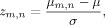
(8)
Investigation of Cortical Dynamics: Local Scale
In the context of MEEG source maps, and because the local velocity vectors V(p,t) are available wherever the corresponding neural sources have been estimated—which may extend over the entire cortical surface or brain volume—the cortical flow measures open a large variety of approaches to the analysis of brain dynamics at a more local scale.
As a matter of illustration and proof of concept, we will focus on the possible correspondence between the speed and direction of the flow of neural activations within the visual cortex and those of the dynamical properties of the stimulus itself in the subject's visual field. Such approach can be extended to other optical‐flow based measures and functional systems: the message being here that velocity‐based measurements complement the more classical amplitude‐based indices of brain activity on the methodological palette of neuroimaging investigators.
Experimental Material
We first illustrate the global approach as applied to MEG data being recording in a ball catching experiment in seven subjects, the results of which have recently been reported elsewhere [Senot et al., 2005, 2008]. In this paradigm, the subjects were required to either catch (catch condition) with their dominant hand or just watch (watch condition) a free‐falling tennis ball while sitting under the MEG sensor array. This study will help illustrate the concept of cortical flow that unfolds with time as it is supposed to elicit a variety of spatially‐distributed brain systems involved in the perception and action relating to moving objects in the subject's visual field.
In this experiment, the event defining the trigger of the evoked field is the release of a tennis ball entering the subject's visual field at time 0 s. One hundred experimental trials were repeated in each condition, and MEG data were time‐locked averaged for each subject. The time window of interest to the analysis ranged from −500 ms to +600 ms about ball release (see [Senot et al., 2008] for detailed description and analysis of the original materials and methods).
We then illustrate the utilization of local cortical flow indices through the estimation of effective propagation of brain responses across primary visual areas. Indeed, by investigating some basic properties of local indices of the cortical dynamics as revealed by MEEG source imaging and subsequent optical flow computation, it is possible to study its correspondence with the kinetic properties of moving objects in the subject's visual field and those of the dynamics of propagation of cortical currents in response to stimulation.
The task being used is visual stimulation using expanding checkerboard rings (see Fig. 1) reaching from 0 to 4 degrees of solid angle and a 5 Hz refresh rate between images. Such stimulation is known to produce steady state activities in localized parts of the visual cortex (see [Cosmelli et al., 2004] for details on the experiment).
Figure 1.
Sequence of expanding rings looped at 5 Hz used for steady‐state visual stimulation.
A seed for a region of interest (ROI) located at the most posterior termination of a subject's calcarine sulcus has been identified from his T1‐weighted magnetic resonance imaging (MRI) brain volume (see Fig. 6). The ROI was further defined automatically from this seed point by diffusing the selection of ROI points forward along the posterior‐to‐anterior direction along the calcarine fold under concavity constraints. ROI growth was terminated once the entire calcarine fold was covered (see Fig. 6). Statistics of the cortical velocity flow field restricted to the calcarine ROI were subsequently extracted and compared with the physical properties of the stimulus.
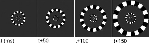
Figure 6.
Instantaneous amplitudes of local velocity vector flow of neural activations along the calcarine sulcus. The colors of the curves encode for the distance to the most posterior part of the calcarine sulcus, as shown in Figure 7.
In both experiments, the optical flow velocity fields were computed from the cortical current distribution estimated using BrainStorm (http://neuroimage.usc.edu) over the individual cortical surface of each subject. Cortical surface segmentation and tessellation from T1‐weigthed axial scans (1 × 1 × 1 mm3 voxel size) was obtained using brainVISA (http://brainvisa.info).
RESULTS
Mapping Global Dynamics Using the Optical Flow
Figure 2 displays the Z m,n arrays summarizing the cross‐correlograms between the MEG surface data topographies in the catch and watch experimental conditions across the group of seven subjects. After identification of microstates and transitions at the sensor level, and according to the methodology described in “Proposition for inferring global brain dynamics at the group level” Section, the event‐related time interval was subsequently divided into 50 sub‐intervals (dt max = 58 ms in the catch condition and dt max = 54 ms in the watch condition) in order to consider the same number of time bins in each condition. Figure 3 complements the illustration of the group analysis of global flow measures using cross‐correlograms computed at the source level. The parallel study of flow dynamics across subjects at the sensor and cortical levels reveals global similarity between cross‐correlograms, at the group level.
Figure 2.
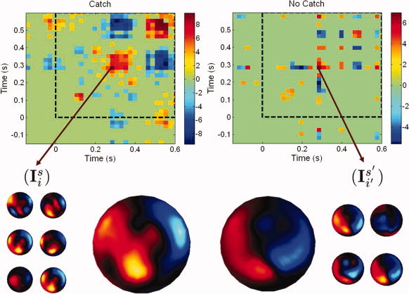
Cross‐correlograms of the spatial topography of MEG sensor data microstates as defined from the cortical flow technique. First row: cross‐correlogram arrays for the catch and watch experimental conditions. The dotted squares indicate the post‐stimulation time frame (i.e., after the free‐falling tennis ball has been released and enters the subjects' visual fields). Second row: left (resp. right), 6 (resp. 4) MEG scalp topographies associated to a temporal interval defined about 300 ms after the ball release in both experimental conditions. The corresponding average sensor topographies is shown at center‐right and center‐left.
Figure 3.
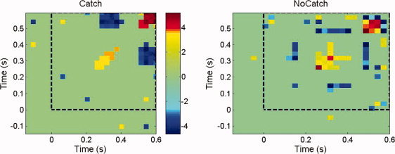
Group level cross‐correlogram [Z m,n] arrays in the catch and watch experimental conditions obtained from optical flow analysis at the source level. See Figure 2 for other legend items.
Strong spatial correlation between microstates across the group of seven subjects can be readily detected about 300 ms after the ball release in the catch condition only. This latency corresponds to the time of flight of the falling ball, which is when subjects catch it with their right hand. Significant cross‐subject correlation of scalp and source patterns was also detected at about 450 ms after ball release, also in the catch condition only. Note the corresponding spatial patterns were found being in anticorrelation with those at 300 ms, thereby indicating similar activity maps but with opposite cortical current flow. The analysis further revealed that cross‐subject spatial correlation of brain activity also occurred at about the time when the ball was released with respect to the sensori‐motor response at the time of catching. This might reveal early build‐up of motor preparation while subjects had been expecting another ball release [Senot et al., 2008].
A closer investigation of the activation patterns occurring at about 300 ms after ball release in the catch (resp. watch) conditions lets us extract the 6 (resp. 4) corresponding individual MEG sensor topographies I (see Section “Proposition for inferring global brain dynamics at the group level”) and their corresponding group averages. Again, visual inspection of the cross‐correlogram arrays allows to quickly determine the regularity of the responses across subjects and the possible differences between experimental conditions at the group level.
Local Directionality of Neural Information
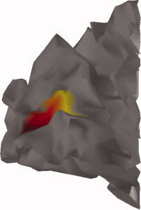
Figure 4 displays a map of MEG distributed source activities restricted to the posterior part of the left hemisphere of a subject during visual stimulation using the expanding ring paradigm.
Figure 4.
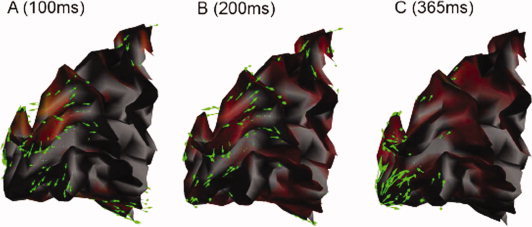
Sagittal views of the posterior portion of white‐grey matter interface the left mesial occipital lobe of one subject during the early response of the expanding rings protocol: the optical flow vector field is shown with green arrows at three different time latencies. The corresponding MEG current source density is shown in a light red shade.
The optical flow of source amplitude constrained to the cortical manifold is represented using green arrows at each time sample. Though visualization of the current flow has its own share of practical interest, we hereby suggest a quantitative evaluation of the local displacement of cortical currents as a new marker of brain activity complementary to the measurement of current amplitude variations.
As a matter of proof of concept, let us consider a point p located within the calcarine fissure where the local kinetic energy integrated over time was found to be maximal in response to stimulation of the subject's visual field. Figure 5 displays the trajectory of the instantaneous velocity vector defined in the local tangent plane to the cortical surface at p. This plot summarizes the changes in direction of the local current flow during different episodes of interest: baseline, transient and steady‐state visual response.
Figure 5.
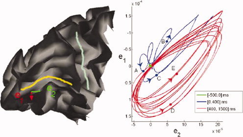
Left: sagittal mesial view of the occipito‐parietal lobe of the left hemisphere of one subject. The calcarine and parieto‐occipital sulci are delineated in yellow and light blue, respectively. e1 and e2 are basis vectors of the local tangent plane at a point p where the norm of the flow vector was found being maximal. Right: trajectory of the flow vector in the tangent plane (p, e1, e2) as the brain activity unfolds in response to visual stimulation using the sequence shown in Figure 1. Colors and five representative points illustrate different segments of the brain response: A:100 ms, B:200 ms, C:365 ms, D:577 ms, and E:977 ms. Segment in green corresponds to baseline brain fluctuations during 500 ms pre‐stimulus; segment in blue illustrates the 400‐ms transition period immediately after stimulation begins; segment in red is an illustration of the established steady‐state response up to the first 1,500 ms after stimulus onset.
Following results communicated in [Cosmelli et al., 2004], the visual steady‐state responses—where the cortical currents in the calcarine area lock to the stimulus refresh rate (5 Hz)—occur within 1.5 s after stimulus onset. A period of transition can be identified immediately following stimulus onset. Figure 5 reveals that the steady‐state velocity plot described a regular, elliptic shape which accounts for the anisotropic directionality of the current flows in this area of the cortex. As expected from the sequential stimulation of various eccentricities in the subject's visual field, the principal direction of neural current corresponded was found lying along the antero‐posterior axis of the calcarine fissure. This is illustrated explicitely Figure 5 after realignment of the respective principal axes of the elliptic trajectory of the flow and of the anatomical fold.
Figure 6, in association with Figure 7, displays the time‐evolution of the instantaneous velocity of current flow along the calcarine fold between −0.5 and 1.5 s about stimulus onset, and reveals changes in velocity amplitudes with distance to fovea. Figures 8 and 9 further complement these measures during steady‐state response and reveal that the average velocity of cortical current propagations tended to decrease with distance to the most posterior part of the calcarine fissure. Such trend was not found during the transition regime where the evolution curve of local instantaneous velocity vectors was found to be near‐flat.
Figure 7.
Colormap of the distances along the calcarine sulcus to its most posterior extremity, as used in Figure 6.
Figure 8.
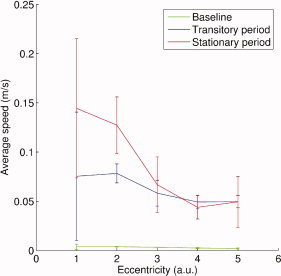
Variation of average flow velocity of cortical currents in the most posterior part of the calcarine fissure in the left hemisphere with stimulus eccentricity. The three curves correspond to baseline (in green), 0–400‐ms transition period (in blue), and up to 1,500 ms after the steady‐state response is established (in red).
Figure 9.
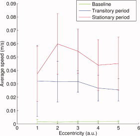
Variation of average flow velocity of cortical currents in the most posterior part of the calcarine fissure in the right hemisphere with stimulus eccentricity. The three curves correspond to baseline (in green), 0–400‐ms transition period (in blue), and up to 1,500 ms after the steady‐state response is established (in red).
DISCUSSION
Global Analysis and the Brain Microstates Revisited
Approaching the concept of brain microstates through a different, more direct, operational hypothesis than in [Pascual‐Marqui et al., 1995] has been the objective of this research. Beyond the different underlying hypothesis leading to the detection of a microstate of relative stability in time, we introduced the definition of transition periods in between two consecutive microstates. Applying the concept of the optical flow to this endeavor at either the sensor or source levels has led us to suggest a natural definition for microstates and transition events. In this contribution, they are defined as local minima (respectively, maxima) of a global kinetic energy index of brain activity. This identification process is essentially non‐parametric and does not necessitate the post‐hoc evaluation of an optimal number of microstates as exhibited from e.g., general cross validation procedures. An immediate benefit to the investigator is the reduction of the density of information carried by MEEG sensor or source data. In the illustrative context of the catch/watch experiment, 625 time samples reporting on 500 ms of brain activity were summarized through about 20 episodes of relative stability of the surface/source data for each subject.
In that respect, we have suggested that temporal cross‐correlograms at the group level would yield a synoptic view of the temporal structure through e.g., reoccurring spatial patterns of MEEG sensor data and source maps across subjects.
An important point of discussion concerns the added value of source imaging of MEEG data to the identification of semi‐stable and transition episodes of brain activity. The optical flow being a non‐linear index derived from amplitude variations, one might expect to extract different temporal structures whether the analysis is completed at the sensor or the cortical source level. We were not expecting any significant added value in that respect in this contribution as the stability and transition nature of any particular episode has been defined according to the variations of DE(t), a summarizing dynamical index defined at the global scale of the measurement manifold. This is illustrated by the similarity between temporal cross‐correlograms defined either at the sensor or the source levels. To take full advantage of the spatial deconvolution brought by MEEG source imaging, new, possibly locally‐defined, indices of the kinetics of cortical currents still remain to be instantiated. We anticipate this is a new opportunity to see computational models reconcile with basic electrophysiology.
Investigation of Local Velocity Fields in the Retinotopic Cortex
Our results have shown how the local average velocity of cortical current flows varied along the calcarine fissure. This raises the question of the physiological relevance of such finding with respect to the expected brain responses to visual simulations with increasing eccentricity. The calcarine fissure is an anatomical landmark of the primary visual cortex which has been found to respond preferentially to stimulation of the horizontal meridians of the visual field. Though the expanding‐rings stimulus we have used obviously elicited a larger portion of the primary and other visual cortices, we have focused our analysis to the calcarine fissure for it marks a clear correspondence between anatomy and the expected brain responses to stimulation.
To discuss the relevance of the variation of local velocity of cortical currents along the calcarine, we refer to a model relating the eccentricity θ of stimulation in the visual field to the distance to the fovea representation l:ln θ = Al + l 0 as suggested in e.g., [Engel, 1997]; [Qiu et al., 2006]; [Wandell, 1999]. Another quantity of interest in this experimental context consists of the linear cortical magnification factor. This latter corresponds to the change in the cortical distance between brain responses respectively elicited by a step of one unit degree of solid angle in the subject's visual field:
We derive from this expression the velocity
 of neural activations within the primary visual areas
| (9) |
Under the assumption that the time evolution of stimulus eccentricity
 is constant, Eq. (9) indicates that the velocity
  is constant in time and decreases with distance to fovea.
This prediction is confirmed by our preliminary results reported on Figure 8, where the average velocity of cortical current flow during steady‐state brain response decreases with stimulus eccentricity, hence distance to the cortical representation of fovea. In a nutshell, at the most local scale under investigation in the present contribution, the parallel between stimulus increase in eccentricity and propagations of cortical currents along the calcarine fold builds from findings from fMRI retinotopic studies (see e.g., [Wandell, 1999]) and suggests MEG source imaging may open a dynamical approach to the study of the retinotopic organization of the human visual system.
From transient to steady‐state brain response, we note that the variance of the instantaneous average velocity of cortical currents in the calcarine region tends to increase as an attractor‐like shape of optical flow trajectory starts to emerge as illustrated in Figure 5. Such a behavior characterizes stereotypical attractors as defined from the theory of dynamical systems. This latter offers a sound framework to investigate the brain as a structured domain on which phenomena take place quasi‐continuously in time. This approach is well exemplified by the school of synergetics as developed by Herman Haken and collaborators. Their theoretical framework predicts for instance that innovation in a global, interconnected system such as the brain cannot be reduced to behaviors at the smallest scales and implies the emergence of persistent, structured spatio‐temporal patterns that are observable at larger scales (see e.g., [Haken, 2006]). We anticipate that semi‐stable and transitory states as revealed by the estimation of the cortical flow of activity may contribute to the experimental body of evidence in favor of this theory.
As a word of caution however, optical flow has been applied electromagnetic brain measures considering a simplistic model that conserves the net, global neural intensity with time. More advanced model for global neural assemblies may be considered in future incarnations of the cortical current flow. In neural fields models elaborated by Jirsa et al. [ 2002] for instance, the equation of neural activities is expressed as the contribution of both local propagation and non‐linear dependence on spatial connectivity. We anticipate however that the model derived in the present contribution provides a reasonable first approximation in terms of directionality of local neural current flows, which is not the case for the model derived in [Jirsa et al., 2002]. Furthermore, the topological structure supported by the vector fields obtained from optical flow estimation might contribute to the identification of sources or sinks of neural activities and derive a spatiotemporal map of directional interactions across the cortical mantle through cortico‐cortical connections and white‐matter fiber tracks Yogarajah and Duncan, 2008].
CONCLUSIONS
We have proposed two applications of the cortical flow, a technique we have adapted from optical flow, to the identification of brain dynamics. We first revisited the concept of microstates through an operational hypothesis relating directly to the kinetics of MEEG sensor topography or cortical currents. By doing so, a natural definition of transition episodes between two brain microstates has been proposed. We also suggested how spatial cross‐correlograms of microstate topographies may help investigate major effects in brain dynamics at the group level. The approach was illustrated by the application to the practical review of experimental data across subjects and conditions. The second application focused on the usage of cortical flow at a more local scale by demonstrating stimulus‐related directionality effects in accordance with the retinotopic organization of visual responses along the calcarine sulcus.
REFERENCES
- Baillet S,Mosher JC,Leahy RM ( 2001): Electromagnetic brain mapping. IEEE Signal Process Mag 18: 14–30. [Google Scholar]
- Blixt EM,Semeter J,Ivchenko N ( 2006): Optical flow analysis of the aurora borealis. Geoscience Remote Sensing Lett, IEEE, 3: 159–163. [Google Scholar]
- Ciarlet PG ( 2002): Finite Element Method for Elliptic Problems. Society for Industrial and Applied Mathematics; Philadelphia, PA, USA. [Google Scholar]
- Corpetti T,Mémin E,Pérez P ( 2002): Dense estimation of fluid flows. IEEE Trans Pattern Anal Machine Intell 24: 365–380. [Google Scholar]
- Cosmelli D,David O,Lachaux JP,Martinerie J,Garnero L,Renault B,Varela F ( 2004): Waves of consciousness: Ongoing cortical patterns during binocular rivalry. Neuroimage 23: 128–140. [DOI] [PubMed] [Google Scholar]
- Engel SA ( 1997): Retinotopic organization in human visual cortex and the spatial precision of functional MRI. Cerebral Cortex 7: 181–192. [DOI] [PubMed] [Google Scholar]
- Freeman WJ ( 2000): Neurodynamics: An Exploration of Mesoscopic Brain Dynamics. London: Springer‐Verlag. [Google Scholar]
- Freeman WJ ( 2006): A cinematographic hypothesis of cortical dynamics in perception. Int J Psychophysiol 60: 149–161. [DOI] [PubMed] [Google Scholar]
- Haken H ( 2006): Synergetics of brain function. Int J Psychophysiol 60: 110–124. [DOI] [PubMed] [Google Scholar]
- Horn BKP,Schunck BG ( 1981): Determining optical flow. Artif Intell 17: 185–204. [Google Scholar]
- Jirsa VK,Jantzen KJ,Fuchs A,Kelso JAS ( 2002): Spatiotemporal forward solution of the EEG and MEG using networkmodeling. Med Imaging IEEE Trans, 21: 493–504. [DOI] [PubMed] [Google Scholar]
- Key AP,Dove GO,Maguire MJ ( 2005): Linking brainwaves to the brain: An ERP primer. Dev Neuropsychol 27: 183–215. [DOI] [PubMed] [Google Scholar]
- Lefèvre J,Baillet S ( 2008): Optical flow and advection on 2‐riemannian manifolds: A common framework. IEEE Trans Pattern Anal Machine Intell 30: 1081–1092. [DOI] [PubMed] [Google Scholar]
- Lefèvre J,Obozinski G,Baillet S ( 2007): Imaging brain activation streams from optical flow computation on 2‐riemannian manifold. Proc Inform Process Med Imaging 4584: 470–481. [DOI] [PubMed] [Google Scholar]
- Lehmann D,Skrandies W ( 1984): Spatial‐analysis of evoked‐potentials in man: a review. Prog Neurobiol 23: 227–250. [DOI] [PubMed] [Google Scholar]
- Michel CM,Seeck M,Landis T ( 1999): Spatio‐temporal dynamics of human cognition. NIPS 14: 206–214. [DOI] [PubMed] [Google Scholar]
- Murray MM,Brunet D,Michel CM ( 2008): Topographic ERP analyses: A step‐by‐step tutorial review. Brain Topogr 20: 249–264. [DOI] [PubMed] [Google Scholar]
- Neumann B ( 1984): Optical flow. Comput Graph 18: 17–19. [Google Scholar]
- Pascual‐Marqui RD,Michel CM,Lehmann D ( 1995): Segmentation of brain electrical activity into microstates: Model estimation and validation. IEEE Trans Biomed Eng 42: 658–665. [DOI] [PubMed] [Google Scholar]
- Qiu A,Rosenau BJ,Greenberg AS,Hurdal MK,Barta P,Yantis S,Miller MI ( 2006): Estimating linear cortical magnification in human primary visual cortex via dynamic programming. Neuroimage 31: 125–138. [DOI] [PubMed] [Google Scholar]
- Schnorr C ( 1991): Determining optical flow for irregular domains by minimizing quadratic functionals of a certain class. Int J Comput Vision 6: 25–38. [Google Scholar]
- Senot P,Zago M,Lacquaniti F,McIntyre J ( 2005): Anticipating the effects of gravity when intercepting moving objects: Differentiating up and down based on nonvisual cues. J Neurophysiol 94: 4471–4480. [DOI] [PubMed] [Google Scholar]
- Senot P,Baillet S,Renault B,Berthoz A ( 2008): cortical dynamics of anticipatory mechanisms in interception: A neuromagnetic study. J Cogn Neurosci 20: 1827–1838. [DOI] [PubMed] [Google Scholar]
- Wandell BA ( 1999): Computational neuroimaging of human visual cortex. Annu Rev Neurosci 22: 145–173. [DOI] [PubMed] [Google Scholar]
- Yogarajah M,Duncan JS ( 2008): Diffusion‐based magnetic resonance imaging and tractography in epilepsy. Epilepsia 49: 189–200. [DOI] [PubMed] [Google Scholar]