Comparison of piece‐wise linear, linear, and nonlinear atlas‐to‐patient warping techniques: Analysis of the labeling of subcortical nuclei for functional neurosurgical applications

Abstract

Digital atlases are commonly used in pre‐operative planning in functional neurosurgical procedures performed to minimize the symptoms of Parkinson's disease. These atlases can be customized to fit an individual patient's anatomy through atlas‐to‐patient warping procedures. Once fitted to pre‐operative magnetic resonance imaging (MRI) data, the customized atlas can be used to plan and navigate surgical procedures. Linear, piece‐wise linear and nonlinear registration methods have been used to customize different digital atlases with varying accuracies. Our goal was to evaluate eight different registration methods for atlas‐to‐patient customization of a new digital atlas of the basal ganglia and thalamus to demonstrate the value of nonlinear registration for automated atlas‐based subcortical target identification in functional neurosurgery. In this work, we evaluate the accuracy of two automated linear techniques, two piece‐wise linear techniques (requiring the identification of manually placed anatomical landmarks), and four different automated nonlinear atlas‐to‐patient warping techniques (where two of the four nonlinear techniques are variants of the ANIMAL algorithm). Since a gold standard of the subcortical anatomy is not available, manual segmentations of the striatum, globus pallidus, and thalamus are used to derive a silver standard for evaluation. Four different metrics, including the kappa statistic, the mean distance between the surfaces, the maximum distance between surfaces, and the total structure volume are used to compare the warping techniques. The results show that nonlinear techniques perform statistically better than linear and piece‐wise linear techniques. In addition, the results demonstrate statistically significant differences between the nonlinear techniques, with the ANIMAL algorithm yielding better results. Hum Brain Mapp, 2009. © 2009 Wiley‐Liss, Inc.

INTRODUCTION

Functional neurosurgical procedures used to treat the symptoms of Parkinson's disease and other movement disorders require careful identification of subcortical surgical targets. These procedures include creation of lesions in the thalamus (thalamotomy) [Atkinson et al., 2002; Duval et al., 2005; Lenz et al., 1995; Otsuki et al., 1994], the globus pallidus (pallidotomy) [Cohn et al., 1998; Gross et al., 1999; Lombardi et al., 2000; Starr et al., 1999] as well as the introduction of deep brain stimulation (DBS) electrodes in the thalamus, globus pallidus, or the subthalamic nucleus (STN) [Bardinet et al., 2005; Chakravarty et al., 2006b; D'Haese et al., 2005a, b; Eskandar et al., 2001; Guo et al., 2005; Krause et al., 2001; Sanchez Castro et al., 2005; Starr et al., 1999]. Despite recent advances in medical imaging techniques, which allow improved visualization of the thalamus [Behrens et al., 2003; Deoni et al., 2005; Johansen‐Berg et al., 2005] and the STN [Bejjani et al., 2000; Benabid et al., 2002; Starr et al., 1999], most clinical magnetic resonance imaging (MRI) volumes lack the adequate contrast and resolution required to properly visualize these subcortical subnuclei (particularly in the thalamus). In addition, to establish a coordinate system within the patient's head, volumes may be acquired with a stereotactic head‐frame attached to the patient's skull. The size of the head‐frame may necessitate the use of a body coil during MRI acquisition, resulting in a further reduction of contrast‐to‐noise ratio. This affects the surgeon's ability to distinguish different subcortical nuclei directly for surgical planning (see Fig. 1).

Figure 1.

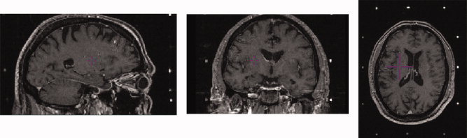
Example of pre‐operative MRI volume with headframe affixed to patient. Left: Sagittal view. Middle: Coronal view. Right: Axial view. Image volume shows lack of contrast in the subcortical nuclei. Surgical targeting is extremely difficult in these nuclei as a result. [Color figure can be viewed in the online issue, which is available at www.interscience.wiley.com.]

Originally, print atlases based on anatomical and histological data were used to guide functional neurosurgical procedures [Ono et al., 1990; Schaltenbrand and Wahren, 1977; Talairach and Tournoux, 1988]. However, digital atlases have proven to be useful in surgical planning and guidance as they can be customized to pre‐operative patient data. Digital atlases of the thalamus and basal ganglia are often used to enhance pre‐operative data and to suggest the location of subcortical targets [Bardinet et al., 2005; Bertrand, 1982; Bertrand et al., 1973, 1974; Chakravarty et al., 2005, 2006b; D'Haese et al., 2005a, b; Finnis et al., 2003; Ganser et al., 2004; Guo et al., 2005; Nowinski et al., 1997, 2000; St‐Jean et al., 1998; Xu and Nowinski, 2001].

Typically atlas‐to‐patient transformations used to customize the atlas‐to‐patient MRI data are estimated using one of two methods. The first is a direct atlas‐to‐patient registration of a reconstructed print atlas, where anatomical structures on the atlas are directly matched to the same structures in pre‐operative images [Ganser et al., 2004; Nowinski et al., 2000; Xu and Nowinski, 2001]. This type of digital atlas creation and warping was pioneered at the Montréal Neurological Institute in work done by Bertrand, Olivier, and Thompson [Bertrand et al., 1973, 1974; Bertrand, 1982] in the early 1970s. In their original work, a digitized version of the Schaltenbrand and Bailey atlas [Schaltenbrand and Bailey, 1959] was matched directly to an intra‐operative ventriculogram imaging reference. The second atlas‐to‐patient customization method starts with a set of anatomical atlas contours, pre‐aligned to an MRI template. A transformation is then estimated between the template MRI and patient's MRI. Once this template‐to‐patient transformation is estimated, the transformation is then applied to the anatomical atlas contours, thus customizing it to patient's anatomy. Thus the atlas‐to‐patient registration problem is reduced to matching an atlas to a template MRI (estimated only once) and is followed by a standard MRI‐to‐MRI registration problem (for each patient) [Bardinet et al., 2005; Chakravarty et al., 2005; D'Haese et al., 2005b; Sanchez Castro et al., 2006; Yelnik et al., 2007].

Recent work has examined the accuracy of different registration techniques used to estimate the atlas‐to‐patient transformation. Bardinet et al. [ 2005] reconstructed a set of serial histological data and warped this data set to T1‐ and T2‐weighted reference MRIs using only linear transformations. Contours of structures in the basal ganglia and the mesencephalon were manually traced on the histology to allow for improved visualization of the anatomy. The atlas was then customized to patient pre‐operative data and used to predict the location for the implantation site of the STN DBS stimulator. Using a hierarchical registration strategy, a rigid body transformation was estimated to match the template MRI to the patient MRI. The transformation was then improved by estimating a subsequent affine transformation matching the cropped region of the basal ganglia and thalamus. The target location suggested by the atlas was then correlated with intra‐operative electro‐physiological findings to evaluate the accuracy of the atlas customization. This group recently reported details of the techniques used for the acquisition and the reconstruction of the histological data used to create the atlas [Yelnik et al., 2007].

D'Haese et al. [ 2005b] have developed an atlas using electro‐physiological intra‐operative recordings from the STN registered to a template created from the average of pre‐operative data. This choice of template was later refined [D'Haese et al., 2005a] to a single MRI template based on the best prediction of the final DBS location when using a warping algorithm based on radial basis functions to estimate the nonlinear template‐to‐patient transformation [Rohde et al., 2003].

The use of expert identification of surgical targets was used to create an atlas for STN DBS targeting by Sanchez Castro et al. [ 2005, 2006], in which two experts manually identified the ideal location for STN DBS placement on clinical MRI data. The raters repeated the labeling on five separate occasions to minimize intra‐rater error. The final atlas was created by averaging the optimal target points and then transforming the average position to a single pre‐operative MRI reference volume. Four different registration techniques were evaluated (Schaltenbrand and Wahren [ 1977], affine transformations [Maes et al., 1997], Demons [Thirion, 1998], and B‐splines [Rueckert et al., 1999]). The quality of atlas‐to‐patient transformations was assessed using the correspondence to the actual target point identified in post‐operative data. Their study found that the Demon's algorithm was most accurate when adapted to match semi‐automated segmentations of easily identified surrounding structures (the lateral and third ventricles, and the inter‐peduncular cistern).

Though not in the context of atlas warping, other evaluations of registration techniques have been performed. Robbins et al. [ 2004] used the minimization of entropy between segmented MRI volumes as a technique for the optimization of nonlinear registration parameters of the automatic nonlinear image matching and anatomical labeling algorithm (ANIMAL) of Collins et al. [Collins and Evans, 1997; Collins et al., 1995]. In a broader study, Hellier et al. [ 2003] studied the accuracy of commonly‐used nonlinear registration techniques using several different criteria including: global volume, overlap of different segmented tissue classes, curvature of the iso‐intensity surfaces, consistency of the nonlinear deformation, as well as quantitative and qualitative evaluation of sulci after nonlinear warping.

Despite the availability of nonlinear atlas customization techniques, subcortical target identification in functional neurosurgical procedures is often performed using one of two methods: (1) semi‐automatically estimated linear or piece‐wise linear transformations [Nowinski et al., 2003] or (2) through the manual identification of targets with respect to absolute distances from easily identified subcortical landmarks (e.g., the midpoint of the anterior commissure or the red‐nucleus) [Benabid et al., 2002; Schaltenbrand and Wahren 1977]. The goal of this work was to compare eight different techniques for atlas‐to‐patient warping to demonstrate the value of nonlinear registration techniques by determining which transformation model provides the most accurate atlas‐based identification of subcortical structures normally targeted in functional neurosurgical procedures.

While a comparison of all possible registration procedures is beyond the scope of this paper, we focus on eight registration strategies here. These include two linear, two piece‐wise linear and two nonlinear techniques that are compared to two variants of our ANIMAL nonlinear registration algorithm [Collins and Evans, 1997; Collins et al., 1995]. The two linear techniques use 9‐parameter (3 translation, 3 rotation and 3 scales) and 12‐parameter (3 translation, 3 rotation, 3 scales, and 3 shears) affine mappings since these transformation models are most often used for linear transformations in many publicly available software packages such as SPM [Friston et al., 1995], FSL tools [Smith et al., 2004], AIR [Woods et al., 1998a, b] and the mni_autoreg MINC toolbox [Collins et al., 1994, 1995; Neelin et al., 1998]. The two manual piece‐wise linear techniques include the classic landmark‐based Talairach mapping [Talairach and Tournoux, 1988] and Nowinski's implementation [Nowinski et al., 2003]. The former was chosen because it was the standard procedure for target planning and continues to be used in many centers. The latter was chosen because it is similar to targeting techniques reliant on the manual identification of subcortical landmarks used in many centers [Benabid et al., 2002]. Since linear transformations cannot account for all possible anatomical variability, we wanted to evaluate the improvement in targeting accuracy when using nonlinear transformations. We choose to include the cosine‐basis function based procedure of SPM [Friston et al., 1995a] because it is one of the most cited techniques in the literature and many readers will be familiar with its performance. We included Hellier's ROMEO technique [Hellier et al., 2001], because it has already been compared to ANIMAL [Collins et al., 1995], Demons [Thirion, 1998], inverse consistent linear elastic registration [Christensen and Johnson 2001] and others. Finally, we included two optimized versions of our ANIMAL procedure [Collins and Evans, 1997; Collins et al., 1995]. We did not include other nonlinear techniques here because (1) our goal was to show that in general, nonlinear techniques are better than linear or piece‐wise linear transformation models, and (2) we did not have expertise to tune other algorithms, and thus felt that a comparison with the optimized version of ANIMAL might be unfair.

Given that a proper gold standard for inter‐subject registration is ill defined, we decided to use structure alignment to evaluate the different registration strategies. In many clinical situations surgeons, residents, or technicians manually identify subcortical structures and targets during the pre‐operative planning process. As such, manually labeled structures definitions from eight pre‐operative MRI volumes were used to create silver standards for evaluation purposes. Labels of the globus pallidus, striatum, and thalamus from a digital atlas of the subcortical nuclei [Chakravarty et al., 2006a] (see below) were customized using six different fully‐automated and two semi‐automated techniques and subsequently evaluated against the silver‐standards. This evaluation criterion along with the use of real pre‐operative data follows the suggestions of Jannin et al. [ 2006] for the validation and evaluation of different medical image processing algorithms and techniques in the clinical context. In their work they advocate close mimicry of the intended clinical situation during the evaluation process.

METHODS

In this section, the digital atlas, the different registration techniques, and the evaluation criteria are described.

Atlas of the Basal Ganglia and Thalamus

For structure identification, a bilateral version of a new high‐resolution anatomical atlas containing multiple registered representations of 105 subcortical grey and white matter structures [Chakravarty et al., 2006a] was used. While it might be possible to use atlases based on manually labeled MRI data, such atlases do not contain the detail needed to identify surgical targets such as subnuclei of the thalamus. The atlas data used here was derived from 84 sections of manually segmented serial histological data. The atlas combines nomenclature from three sources for gross‐anatomy [Schaltenbrand and Wahren, 1977], thalamus [Hirai and Jones, 1989], and temporal lobe [Gloor, 1997]. The histological data used for the atlas was originally reconstructed using the technique described in [Chakravarty et al., 2003] and later optimized in [Chakravarty et al., 2006a]. The multiple representations of the atlas include (1) a set 84 slices of registered histological data, (2) a set of 105 3D geometrical objects representing the anatomical structures of the atlas, and (3) a 3D volume (with 250 × 250 × 250 μm voxels) containing a voxel‐label atlas, where each voxel is assigned a unique label corresponding to the corresponding anatomical structure. All three datasets are defined in the same coordinate system are aligned together.

Since MRI of the anatomical data was not acquired before the histology was prepared, we decided to use the Colin27 average MRI volume as a template for the atlas [Holmes et al., 1998]. The MRI and histological data needed to be registered together, since they did not come from the same source. To estimate the nonlinear atlas‐to‐template transformation, a pseudo‐MRI was created by modifying the intensities of the voxel‐label atlas to match those of the Colin27 average MRI. The ANIMAL algorithm was used to align the atlas pseudo‐MRI data with the real MRI volume, thus registering the atlas data with the Colin27 MRI template [Chakravarty et al., 2006a].

The different atlas representations (histological, voxel‐label, pseudo‐MRI, geometric) can be viewed together or separately. These representations, along with the Colin27 MRI template can be seen in Figure 2. The atlas and our atlas‐to‐template and atlas‐to‐patient warping were chosen because they have recently been validated in [Chakravarty et al., 2008a] and cross‐validated against fMRI activations in [Chakravarty et al., 2008b].

Figure 2.

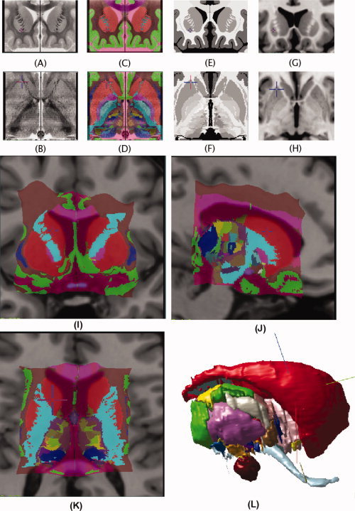
Coronal and axial representation of the atlas described in Atlas of the Basal Ganglia and Thalamus. A: Original coronal section from the histological dataset. B: Reconstructed transverse slice through the histological volume. C, D: Voxel‐label atlas representation of the atlas. E, F: Pseudo‐MRI representation of the atlas. G, H: Close‐up of the Colin27 MRI template in the region of the basal ganglia and thalamus. I–K: Coronal, sagittal, and axial views of the atlas warped to fit the Colin27 template. L: The geometric representation of the atlas that can be manipulated in 3D.

Atlas‐to‐Patient Warping

In order to properly identify the subcortical anatomy of a given patient, the atlas must be customized (or warped) to effectively match the patient's morphology. The linear, piece‐wise linear, and nonlinear techniques evaluated for atlas‐to‐patient warping are described in more detail here.

Linear techniques

The 9‐ and 12‐parameter transforms were used to provide a baseline for all evaluation metrics since such transformation models are used in many publicly available software packages. Our assumption was that regardless of the choice of linear registration algorithm, nonlinear registration would improve the quality of the labeling of subcortical structures.

LSQ9

The different automatic linear transformations were estimated using the optimization scheme available in the mni_autoreg package (packages.bic.mni.mcgill.ca) [Collins et al., 1994]. Both cases start with the estimation of a 7‐parameter linear transformation (3 translations, 3 rotations, and one global scale) that best aligns the source and the target volumes by maximizing the correlation of blurred MRI intensities and gradient magnitude evaluated over the whole brain. Further refinement is achieved by estimating a 9‐parameter transformation through the maximization of the correlation of gradient magnitude data, (again over the whole brain) using a simplex optimization technique. Details of the size of the Gaussian kernel and the type of data used at each step of the fitting procedure are given in Table I.

Table I.

Parameters used to estimate a 9‐parameter and 12‐parameter atlas‐to‐patient transformation

Transformation type	FWHM (mm)	Data used
7	16	Intensity
7	8	Intensity
7	8	Gradient
9	4	Gradient
12	4	Gradient

LSQ12

The nine‐parameter transformation estimated above is used as the starting point to estimate a 12‐parmeter transformation which maximizes the correlation of the gradient data, evaluated over the whole brain. Details of the size of the Gaussian kernel and data used at each step are given in Table I.

Piece‐wise linear techniques

Talairach

The Talairach transformation requires the manual identification of twelve different landmarks on both the atlas and patient data [Talairach and Tornoux 1988]. These 12 landmarks are listed below.

• 1The posterior–superior margin of the anterior commissure (AC).
• 2The anterior–inferior margin of the posterior commissure (PC).
• 3The most superior point of the left parietal lobe.
• 4The most superior point of the right parietal lobe.
• 5The most posterior point of the left occipital lobe (the occipital pole).
• 6The most posterior point of the right occipital lobe (the occipital pole).
• 7The most inferior point of the left temporal lobe.
• 8The most inferior point of the right temporal lobe.
• 9The most anterior point of the left frontal lobe (the frontal pole).
• 10The most anterior point of the right frontal lobe (the frontal pole).
• 11The most lateral point of the left parietotemporal lobe.
• 12The most lateral point of the right parietotemporal lobe.

These landmarks were identified by one of the authors (MMC).

The line passing through the AC and PC landmarks gives the main orientation of the brain. These landmarks are used to divide the brain into two sections in the left‐right direction (between each lateral point defined on the parietotemporal lobes and the AC–PC line). Each of these subvolumes is further divided into two sections in the inferior‐superior direction (from the superior parietal point to the AC–PC line, and from the AC–PC line to the inferior temporal points) and three sections in the anterior‐posterior directions (one region from the frontal pole to the AC, one region between the AC and PC, and one region from the PC to the occipital pole), thus creating a total of 12 piece‐wise linear regions. See Figure 3 for the definition of the AC–PC line, and the 12 regions.

Figure 3.

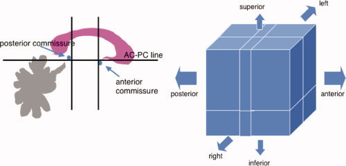
Left: The Talairach definition of the AC–PC line. Also shown are the divisions anteriorly and posteriorly and in the superior–inferior directions. Right: The 12 regions defined by the Talairach proportional grid system. [Color figure can be viewed in the online issue, which is available at www.interscience.wiley.com.]

In our implementation, the patient MRI data is translated and then rotated so the mid‐sagittal plane is parallel and coincident to that of the Colin27 template. Afterwards, the patient data is rotated around the lateral (left‐right) axis going through the AC so that AC–PC line of the patient overlaps with that of the atlas. In each of the 12 regions, the atlas was cropped and scaled in 3D in order to normalize each region of the patient data with respect to the homologous landmarks pairs.

In the Results and the Discussion sections, the abbreviation TAL will be used for the Talairach technique.

Probabilistic functional atlas

The second piece‐wise linear technique was proposed by Nowinski et al. [ 2003] for the creation of a probabilistic functional atlas for neurosurgical planning. The probabilistic functional atlas (PFA) transformation is defined by six different landmarks:

• 1The midpoint of the AC.
• 2The midpoint of the PC.
• 3The most superior point of the left thalamus.
• 4The most superior point of the right thalamus.
• 5The most lateral point left side of the third ventricle.
• 6The most lateral point right side of the third ventricle.

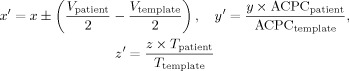
One transformation is estimated for each hemisphere using the following formulae

(1)

where (x′,y′,z′) represents a point in the patient space, (x, y, z) represents a point in the atlas space, and (V _patient, ACPC_patient, T _patient) and (V _template, ACPC_template, T _template) represent the magnitude of the ventricle widths V, the AC–PC line length ACPC and the height of the thalamus T with respect to the AC–PC in the patient and Colin27 template respectively. Here the y and z coordinates are scaled linearly for the size of the thalamus and ACPC line; however there is only an offset in the x direction. Similar to our implementation of the Talairach proportional grid transformation, the patient data is rotated so the mid‐sagittal plane is parallel to that of the Colin27 template and both volumes were rotated around the lateral axis going through the AC and PC so that both AC–PC lines overlap.

We will use the abbreviation PFA for referring to this technique in the Results and Discussion sections.

Nonlinear techniques

For all nonlinear techniques the LSQ9 transformation estimated for each MRI volume was first applied prior to further refinement through nonlinear transformation estimation. This allowed for a common starting point for the four nonlinear registration algorithms evaluated.

SPM

The SPM registration technique refers to the nonlinear registration technique [Friston et al., 1995a] provided in the Statistical Parametric Mapping [Friston et al., 1995b] toolbox (SPM5 was used in the experiments performed). In their approach, a transformation dx matches a source S to a target T volume using a set of smoothly varying spatial basis functions:

(2)

where β${}_{\mathit{\text{q}}}^{\mathit{\text{k}}}$(x) is an expansion of smoothly varying basis functions. The source object can be transformed iteratively using the following first order approximation:

(3)

Although any set of basis functions could be used, the default SPM implementation of the nonlinear registration algorithm uses discrete cosine transform (DCT) and a sixth order expansion for the coefficients estimated at each control node using least‐squares optimization procedure to minimize the sum of squared differences. The default configuration of the registration algorithm was used for all experiments and uses both source and target volumes convolved with an 8 mm Gaussian kernel for transformation estimation.

ROMEO

The Romeo registration method [Hellier et al., 2001] is based on the optical flow hypothesis. The optical flow algorithm expresses the registration process as the minimization of a cost function depending on two terms: a flow‐based similarity measure, and a regularization term. The optical flow hypothesis, introduced by Horn and Schunck [ 1981], assumes that the luminance of a physical point does not change when the point moves with the flow: f(S+d _S,x ₁)−f(S,x ₂) = 0, where S is a voxel of the volume, x ₁ and x ₂ are the indices of the volumes (temporal indices for a dynamic acquisition, indices in a database for multi‐subject registration), f is the luminance function and d the expected 3D displacement field.

Generally, a linear expansion of this equation is preferred: ∇f(S,x)·d _S + f _x(S,x) = 0 where ∇f(S,x) stands for the spatial gradient of luminance and f _x(S,x) is the voxel‐wise difference between the two volumes. The resulting set of undetermined equations has to be complemented with some prior on the deformation field. This prior is defined according to the quadratic difference of the deformation field computed between neighbors. Using an energy‐based framework the regularization problem may be formulated as the minimization of the following cost function:

(4)

where S is the voxel lattice, C is the set of neighboring pairs with respect to a given neighborhood V on S(〈s,r〉∈C ⇔︁ s ∈ V(r)), and α controls the balance between the two energy terms. The first term is the linear expansion of the luminance conservation equation and represents the interaction between the field and the data. The second term is the smoothness constraint. In order to cope with large displacements, a classical incremental multi‐resolution procedure was developed. A pyramid of volumes is constructed by successive Gaussian blurring and subsampling. At the coarsest level, displacements are reduced and the linearization hypothesis (linear expansion of the optical flow hypothesis) can be used. At the subsequent resolution level k, only an increment is estimated and used to refine estimate from the previous level. Furthermore, at each resolution level, a multigrid minimization based on successive partitions of the initial volume is achieved. A grid level is associated to a partition of cubes. At a given grid level l, a piece‐wise affine incremental field is estimated. The resulting field is a rough estimate of the desired solution, and it is used to initialize the next grid level. This hierarchical minimization strategy improves the quality and the convergence rate. For the experiments, the parameter α was set to a relatively high value (5,000) to obtain a regular deformation field.

The abbreviation ROM will be used in the Results and Discussion sections for the ROMEO algorithm.

ANIMAL‐1

The ANIMAL algorithm is an iterative procedure that estimates a 3D deformation field that matches a source volume to a target volume. The algorithm is divided into two steps. The first is the outer loop, where large deformations are estimated on data that has been blurred using a Gaussian kernel with a large full‐width‐at‐half‐maximum (FWHM). These larger deformations are then input to subsequent steps where the fit is refined by estimating smaller deformations on data blurred with a Gaussian kernel with smaller FWHM.

At each step of the outer loop, the ANIMAL algorithm is applied iteratively in an inner loop to optimize the nonlinear transformation (N) that maximizes the similarity between a source volume (S) and a target volume (T) with the following objective function Γ:

(5)

where β is the local similarity measure (i.e., the correlation ratio) and C is the cost function. The cost function yields large values for large deformations and smaller values for smaller deformations, thus effectively penalizing the objective function when large deformations are estimated.

The nonlinear transformation is represented by a deformation field that is iteratively estimated in the inner loop using a two step process: the first step involves the estimation of local translations for each node defined by optimizing Eq. (5) and the second is a smoothing step to ensure that the deformation field is continuous and does not cause stretching, tearing, or overlap. Three parameters can be set which help define the quality of the nonlinear transformation: the similarity (which balances the objective function with the cost function), the weight (which determines the proportion of each local translation estimated at one iteration that will be used at the next iteration), and the stiffness (which determines the smoothness of the nonlinear deformation field). The similarity, weight, and stiffness are all set to the same value for all iterations (0.3, 1, and 1 respectively) according to the parameter optimization of Robbins et al. [ 2004]. The final transformation estimated was defined by vectors on a grid of equally spaced nodes that are 2 mm apart. The reader is referred to [Chakravarty et al., 2006a; Collins and Evans, 1997; Robbins et al., 2004] for more details on these parameters.

ANIMAL‐1 refers to the version of ANIMAL optimized by Robbins et al. [ 2004]. The parameters used at each hierarchical step are summarized in Table II. We will refer to the ANIMAL‐1 technique using the abbreviation A1 in the Results and Discussion sections.

Table II.

ANIMAL parameters used for template‐based atlas‐to‐subject nonlinear transformation estimation in Method ANIMAL‐1

FWHM (mm)	Step size (mm)	Sublattice diameter	Sublattice	Iterations
8	8	24	6	30
8	4	12	6	30
4	2	6	6	10

ANIMAL‐2

Although similar to ANIMAL‐1, ANIMAL‐2 was the final nonlinear technique evaluated. There are two main differences between ANIMAL‐1 and ANIMAL‐2. While the Colin27 template is still used as the source volume, a cropped volume containing only the subcortical nuclei is used to limit the transformation estimation to reduce the computational burden of estimating a higher‐resolution transformation. The hierarchical nonlinear transformation estimation of this technique outputs a final transformation defined by vectors on a grid of equally spaced nodes that are 1 mm apart. The parameters for ANIMAL used for this template‐based transformation estimation are shown in Table III. We hypothesize that ANIMAL‐2 will give better results than ANIMAL‐1 due to the higher resolution deformation.

Table III.

ANIMAL parameters for high‐resolution template‐based atlas‐to‐subject linear transformation estimation in Method ANIMAL‐2

Step	Step size (mm)	Sublattice diameter	Sublattice	Iterations
1	4	8	6	15
2	2	6	6	15
3	1	6	3	15

Evaluation on Clinical Data

The following sections present the anatomical validation data used for each registration technique used in this study.

Subjects

The eight registration techniques used for atlas‐to‐patient warping presented in the previous section were evaluated using clinical T1‐weighted pre‐operative images from 8 patients who had undergone thalamotomies (4 males and 4 females, 4 left and 4 right thalamotomies). All MRIs were taken between 1997 and 2002 with the stereotactic headframe attached using a Philips 1.5T MRI scanner (Best, The Netherlands). Data was acquired with axial slices with a 1 mm in plane voxel spacing and 1.5 mm thick slices with TE = 9 ms and TR = 27 ms. Since the headframe cannot fit inside the headcoil, scans were acquired in the body coil. Informed consent was obtained from all subjects involved in this study, and the ethics board of the Montréal Neurological Hospital and Institute approved the research protocol.

Anatomical validation

Since a gold standard for anatomical validation was not available, manual structure segmentations were used to evaluate the “goodness‐of‐fit” of the atlas‐to‐patient warping techniques. To estimate inter‐rater variability, five expert raters identified the striatum (the caudate nucleus, the putamen, and the nucleus accumbens), the thalamus, and the globus pallidus bilaterally in the patient MRI data. All raters were trained according to rules developed by the authors. As shown in Figure 1, patient scans acquired with the head‐frame in a body coil suffer from a lack of contrast and resolution (making it difficult for the raters to properly label the subcortical nuclei). To aid the raters, the pre‐operative scan used for diagnostic purposes was registered to the head‐frame scan (using a rigid‐body transformation [Collins et al., 1994]) and the two were averaged to improve the signal‐to‐noise ratio and contrast to facilitate the identification of the subcortical nuclei mentioned above.

The abbreviation man will be used to identify the results of manual segmentation in the Results and Discussion sections. When referring to specific manual raters, the abbreviation man1 will be used for Rater 1, man2 will be used for Rater 2 and so forth.

Derivation of a silver standard

In the absence of an anatomical “gold standard” a series of “silver standards” were created from the manual labels in a leave‐one‐out fashion, where a single rater's labels are compared to a silver‐standard developed through the agreement of other labels (as described in Algorithm 1). Essentially, voxels in the silver standard are set to one if at least three of the four raters have labeled the voxel. This was used to evaluate the registration‐based atlas‐to‐patient labeling of the 8 patients.

Algorithm1: Technique for the derivation of the silver standard for five manual raters

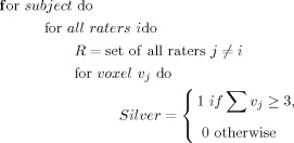Evaluation Metrics

The kappa overlap metric

The labels defined by the atlas or a single rater (defined as the test structure) are compared to a silver standard by determining the level of overlap using the kappa metric (κ):

(6)

where α is the number of voxels common to the test structure and the silver standard, and (b + c) represents the sum of the voxels uniquely identified by either the test structure or the silver standard. The kappa metric was previously used in our validation work done in [Chakravarty et al., 2005, 2008a], where the sensitivity due to simulated error was demonstrated. Typically, κ ≥ 0.7 are deemed acceptable in the segmentation and classification literature, but this value depends on the shape and size of the structure. For objects with a high surface‐to‐volume ratio, a lower value for kappa can be expected.

Distance metrics

Two different metrics based on the chamfer distance [Borgefors, 1984] (an approximation of the more accurate Euclidean distance [Duda et al., 2000]) were used. In both cases, a positively signed distance map (on both the inside and outside of each structure) was estimated using the binary labels for each of the three structures labeled in each of the silver standards. This is similar to the implementation of VALMET of Gerig et al. [ 1998]. Contours were generated from the test structure (data from the manual rater or the labels created by one of the registration algorithms) by using a single 26‐connected voxel erosion of the label data. These border voxels were intersected with the distance maps to compute the two metrics.

The first metric is the mean distance, μ, between the voxel contours generated and the silver standard. This metric gives an idea of how well the structure borders match. Values near zero indicate good agreement.

The second metric is the maximum distance, M, between voxel contours and the silver standard. This metric was used to approximate the symmetric Hausdorff distance. In the case of this metric, we followed the same computation as the symmetric Hausdorff distance: if M ₁ = H(a,b) and M ₂ = H(b,a), where H is the Hausdorff distance, then M = max(M ₁,M ₂).

Total volume

The total volume, V, was also estimated for each of the structures labels identified by the manual raters, the atlas customization techniques and each of the silver standards.

Statistical analysis

The quality of the manual segmentations were first assessed to determine their usefulness as a silver standard. For the kappa and two distance metrics, each of the results of the manual rater and the estimated silver standard were analyzed using an ANOVA. Differences between the volume estimates from each manual rater were also analyzed using an ANOVA. In cases where statistical differences were found between raters, a post‐hoc analysis was done using a Tukey Kramer HSD.

In order to have an equal number of observations, the results of the manual raters were pooled when comparing the atlas warping techniques and the raters. In the analysis of the kappa and distance metrics a repeated‐measures one‐way ANOVA was performed for each structure. The five values estimated using the five silver standards were considered the repeated measurements. Significant differences in the results were once more analyzed using a post‐hoc Tukey Kramer HSD. In this case, the volume measurements from the five silver standards were averaged in order to have the same number of measurements for the silver standard and the atlas‐warping techniques (as each rater has one volume measurement for each structure tested on each subject).

The results of the Tukey Kramer HSD are reported as follows. Methods falling into group A perform with significantly better values than the methods of group B. Similarly, the methods of group B have significantly better values than group C, and so on. This means that the larger values for the kappas will fall into Group A. However for the distance metrics, the lower values will fall into the group A. For the analysis of volume, the groups are ranked in ascending order. Post‐hoc analysis separated results into groups with P < 0.05. A method can be included in multiple groups if it shows no significant difference with one of the methods of each group. All statistical analyses were performed with JMP 5.1.2 (The SAS Institute Inc., Cary, USA).

RESULTS

Manual Raters

Kappa overlap metric

Results for the kappas and the ANOVA (and the post‐hoc Tukey Kramer HSD) for each of the manual raters labels are summarized in Table IV.

Table IV.

Result from post‐hoc Tukey Kramer HSD test for kappas (κ) from raters only

	Globus pallidus		Striatum		Thalamus
Method	Groups	Mean ± SD (range)	Groups	Mean ± SD (range)	Groups	Mean ± SD (range)
Rater 1	A	0.641 ± 0.114 (0.429–0.834)	A, B	0.838 ± 0.029 (0.797–0.895)	B	0.799 ± 0.053 (0.675–0.872)
Rater 2	A	0.684 ± 0.101 (0.441–0.839)	A	0.842 ± 0.025 (0.806–0.890)	A	0.862 ± 0.030 (0.783–0.907)
Rater 3	A, B	0.629 ± 0.119 (0.373–0.809)	B	0.810 ± 0.037 (0.810–0.895)	A	0.849 ± 0.030 (0.786–0.886)
Rater 4	B	0.531 ± 0.112 (0.322–0.732)	B	0.808 ± 0.034 (0.727–0.863)	A, B	0.836 ± 0.048 (0.712–0.885)
Rater 5	C	0.450 ± 0.066 (0.314–0.555)	C	0.746 ± 0.032 (0.746–0.808)	B	0.799 ± 0.036 (0.727–0.851)

Raters are grouped based on the result of Tukey Kramer HSD post‐hoc analysis (P < 0.05). The mean, minimum, maximum, and standard deviations of the kappas are also provided.

The results of the ANOVA for the globus pallidus show significant differences between all raters (F = 13.13, DF = 4, P < 0.001). The results show that Rater 2 has highest mean kappa score (κ_man2 = 0.684). The post‐hoc test shows no differences between raters 1 (κ_man1 = 0.641), 2, and 3 (κ_man3 = 0.629) or between raters 3 and 4 (κ_man4 = 0.531). Rater 5 had significantly lower kappas than all other raters (κ_man5 = 0.450).

The results of the ANOVA results for the striatum also show significant differences between all raters (F = 23.73, DF = 4, P < 0.0001). Results for the striatum once again show that Rater 2 has the highest mean kappa (κ_man2 = 0.842). The post‐hoc Tukey Kramer HSD showed no significant differences were observed between raters 1 (κ_man1 = 0.838) and 2. Rater 1 also showed no significant differences with the results of raters 3 (κ_man3 = 0.810) and 4 (κ_man4 = 0.808). Rater 5 once again has a mean kappa significantly lower than the rest of the raters (κ_man5 = 0.746).

The ANOVA performed on the results for the thalamus demonstrates significant differences in each of the rater's agreement with the silver standard (F = 8.04, DF = 4, P < 0.0001). Once again, the Rater 2 shows highest mean agreement with the silver standard (κ_man2 = 0.862). No significant differences between raters 2, 3 (κ_man3 = 0.849), and 4 (κ_man4 = 0.836). Significant differences were also not observed between the results of raters 1 (κ_man1 = 0.799), 4, and 5 (κ_man5 = 0.799).

Mean chamfer distance

Results for the mean chamfer distance between surfaces of each rater's labels and the silver standard as well as the ANOVA are summarized in Table V.

Table V.

Result from post‐hoc Tukey Kramer HSD test for mean chamfer distance (μ) from raters only

	Globus pallidus		Striatum		Thalamus
Method	Groups	Mean ± SD (range)	Groups	Mean ± SD (range)	Groups	Mean ± SD (range)
Rater 1	A, B	1.72 ± 0.53 (1.16–2.91)	A	1.35 ± 0.28 (1.00–2.16)	B, C	1.67 ± 0.27 (1.25–2.23)
Rater 2	A	1.38 ± 0.34 (1.11–2.42)	A	1.23 ± 0.17 (1.07–1.64)	A, B	1.49 ± 0.23 (1.22–2.11)
Rater 3	A, B	1.76 ± 0.60 (1.15–2.42)	A	1.26 ± 0.17 (1.00–1.63)	A	1.32 ± 0.16 (1.14–1.80)
Rater 4	B, C	2.04 ± 0.50 (1.25–2.97)	A	1.30 ± 0.20 (1.03–1.72)	A, B	1.51 ± 0.26 (1.18–2.21)
Rater 5	C	2.49 ± 0.37 (1.96–3.38)	B	1.66 ± 0.23 (1.30–2.12)	C	1.77 ± 0.28 (1.35–2.44)

Raters are grouped based on the result of Tukey Kramer HSD post‐hoc analysis (P < 0.05). The mean, minimum, maximum, and standard deviations of the mean distances are also provided. All measurements provided in millimeters.

The ANOVA performed on the results of the globus pallidus show significant differences across raters (F = 12.06, DF = 4, P < 0.0001). Rater 2 had lowest mean results (μ_man2 = 1.38 mm). The results for raters 1 (μ_man1 = 1.72 mm) and 3 (μ_man3 = 1.76 mm) were not statistically different from Rater 2. Mean distances for raters 1, 3, and 4 (μ_man4 = 2.04 mm) showed no significant differences, and results for 5 (μ_man5 = 2.49 mm) were not significantly different than those of Rater 4.

Significant differences were observed from the ANOVA performed on the results from the striatum (F = 7.59, DF = 4, P < 0.0001). For the striatum, Rater 2 showed the mean chamfer distance closest to zero (μ_man2 = 1.23 mm). Results from the post‐hoc analysis shows no statistical difference between raters 1 (μ_man1 = 1.35 mm), 2, 3 (μ_man3 = 1.26 mm), and 4 (μ_man4 = 1.30 mm). The results of Rater 5 showed significantly higher error than the other raters (μ_man5 = 1.66 mm).

For the thalamus, the results show significant differences between raters (F = 8.30, DF = 4, P < 0.0001). Rater 3, shows the mean values closest to zero (μ_man3 = 1.32 mm), and the results of post‐hoc test show no significant differences between raters 2 (μ_man2 = 1.49 mm), 3, and 4 (μ_man4 = 1.51 mm). Raters 1(μ_man1 = 1.67 mm), 2, and 4 form a second group. The final group is composed of raters 1 and 5 (μ_man5 = 1.77 mm).

Maximum chamfer distance

Results for the maximum chamfer distance between surfaces of each rater's labels and the silver standards as well as the ANOVA are summarized in Table VI.

Table VI.

Result from post‐hoc Tukey Kramer HSD test for maximum chamfer distance (M) from raters only

	Globus pallidus		Striatum		Thalamus
Method	Groups	Mean ± SD (range)	Groups	Mean ± SD (range)	Groups	Mean ± SD (range)
Rater 1	B, C	6.40 ± 2.69 (3.10–11.98)	A	7.37 ± 2.82 (3.68–14.96)	C	5.74 ± 1.21 (3.68–8.50)
Rater 2	A	3.92 ± 1.42 (2.52–7.73)	A	7.80 ± 3.18 (3.28–15.32)	A, B	4.33 ± 0.56 (2.90–5.36)
Rater 3	C, D	7.88 ± 2.42 (5.02–13.91)	A	8.47 ± 2.80 (4.07–12.94)	A	3.96 ± 0.94 (2.43–5.90)
Rater 4	A, B	5.80 ± 1.37 (3.49–8.37)	A	6.02 ± 2.42 (3.10–12.94)	B, C	5.49 ± 1.46 (3.97–8.46)
Rater 5	D	8.95 ± 2.14 (5.24–13.33)	A	6.83 ± 1.60 (4.45–10.75)	C	5.95 ± 1.50 (4.26–9.85)

Raters are grouped based on the result of Tukey Kramer HSD post‐hoc analysis (P < 0.05). The mean, minimum, maximum, and standard deviations of the maximum distances are also provided. All measurements provided in millimeters.

Results from the ANOVA on the globus pallidus show significant differences between raters (F = 15.41, DF = 4, P < 0.0001). The post‐hoc analysis shows that Rater 2 (M _man2 = 3.92 mm) showed lowest error, but no significant differences with Rater 4 (M _man4 = 5.80 mm). Raters 1 (M _man1 = 6.40 mm) and 4 form the next group, followed by the next group formed by raters 1 and 3 (M _man3 = 7.88 mm). Raters 3 and 5 (M _man5 = 8.95 mm) formed the final group with largest maximum chamfer distance.

The results from the ANOVA showed no significant difference between the raters for the striatum (F = 0.5448, DF = 4, P < 0.7033). The means of maximum chamfer distance are written here in ascending order: Rater 4 (M _man4 = 6.02 mm), 5 (M _man5 = 6.83 mm), 1 (M _man1 = 7.37 mm), 2 (M _man2 = 7.80 mm), and 3 (M _man3 = 8.47 mm).

ANOVA results for the maximum distance values recorded for the thalamus revealed significant differences between raters (F = 9.00, DF = 4, P < 0.0001). Rater 3 showed results closest to zero (M _man3 = 3.96 mm) and the post‐hoc analysis showed no significant difference with Rater 2 (M _man2 = 4.33 mm). Raters 2 and 4 (M _man4 = 5.49 mm) also showed no significant differences between their results. Additionally, no significant differences were observed between raters 1 (M _man1 = 5.74 mm), 4, and 5 (M _man5 = 5.95 mm).

Volumes

The results for the volumes and the ANOVA performed on these results are summarized in Table VII.

Table VII.

Result from post‐hoc Tukey Kramer HSD test for volumes (V) from raters only

	Globus pallidus		Striatum		Thalamus
Method	Groups	Mean ± SD (range)	Groups	Mean ± SD (range)	Groups	Mean ± SD (range)
Rater 1	A	928 ± 266 (448–1564)	A, B	6569 ± 1347 (4043–9050)	C	7207 ± 907 (5715–9331)
Rater 2	A	935 ± 385 (460–2074)	A	5913 ± 1371 (331–8055)	A	5258 ± 873 (3588–7167)
Rater 3	A, B	1083 ± 330 (605–1651)	B	7467 ± 1324 (5114–9359)	A, B	6017 ± 901 (4888–7681)
Rater 4	A, B	1268 ± 304 (829–1872)	A, B	7469 ± 1340 (5644–9758)	B	6248 ± 734 (5151–7714)
Rater 5	B	1363 ± 498 (768–2495)	A	6031 ± 1260 (3515–8206)	A	5305 ± 702 (4138–6632)

Raters are grouped based on the result of Tukey Kramer HSD post‐hoc analysis (P < 0.05). The mean, minimum, maximum, and standard deviations of the maximum distances are also provided. All measurements provided in cubic millimeters.

Significant differences were observed between the volumes of the globus pallidus labeled (F = 4.57, DF = 4, P < 0.0023). Raters 1 (V _man1 = 928 mm³), 2 (V _man2 = 935 mm³), 3 (V _man3 = 1,083 mm³), and 4 (V _man4 = 1,268 mm³) showed no significant differences between their results and form group A. Rater 5 labeled the largest mean volume (V _man5 = 1,363 mm³) and post‐hoc analysis showed no significant difference with the volume labeled by raters 3 and 4.

The results of the analysis on the volume of the manually labeled striatum indicate a significant difference in the volume between all raters (F = 5.03, DF = 4, P < 0.0012). Raters 1 (V _man1 = 6,569 mm³), 2 (V _man2 = 5,913 mm³), 4 (V _man4 = 7,469 mm³), and 5 (V _man5 = 6,031 mm³) show no differences in the structure volumes. Rater 4 shows the highest mean volume over all raters, however the post‐hoc analysis showed no significant differences between raters 1, and 3 (V _man3 = 7,467 mm³).

The ANOVA results indicate significant intra‐rater differences in thalamic volume (F = 14.87, DF = 4, P < 0.0001). Raters 2 (V _man2 = 5258 mm³), 3 (V _man3 = 6,017 mm³), and 5 (V _man5 = 5,305 mm³) showed no significant differences in volume labeled and form the first group. Raters 3 and 4 (V _man4 = 6,248 mm³) show no statistical differences in their results and form the next group. The post‐hoc analysis shows that Rater 1 (V _man1 = 7,207 mm³) labeled a significantly higher volume than the other raters.

Since no manual rater was consistently different from the rest, the silver standards for all raters were used to evaluate the eight warping techniques in the next section.

Evaluation of Atlas Warping Techniques

An example of the results from all manual raters and all warping techniques is included is Figure 4. The figure shows consistent definitions over all structures by the manual raters. Variable definitions of the globus pallidus, medial and posterior borders of the thalamus, and the medial portion of the head of the caudate can also be observed.

Figure 4.

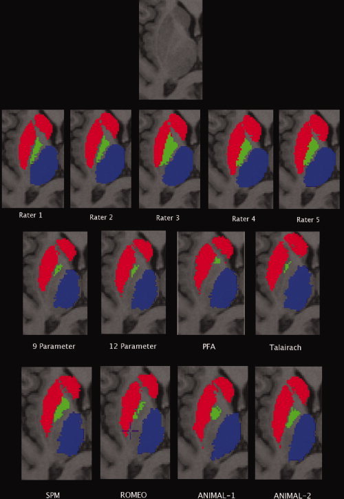
Results of the atlas warping. From top to bottom: Original data unlabeled, result from the data labeled by the five manual raters, results from the linear (LSQ9, LSQ12) and piece‐wise linear (PFA, Talairach) atlas warping, and results from the nonlinear atlas warping (SPM, Romeo, ANIMAL‐1, ANIMAL‐2).

Kappa overlap metric

Results from the kappas and the post‐hoc Tukey Kramer HSD for each structure are shown in Table VIII for all structures and a graphical representation is given in the top panel of Figure 5.

Table VIII.

Result from post‐hoc Tukey Kramer HSD test for kappa (κ) values from raters and all warping techniques for all test structures

	Globus pallidus		Striatum		Thalamus
Method	Groups	Mean ± SD (range)	Groups	Mean ± SD (range)	Groups	Mean ± SD (range)
Manual raters	A	0.587 ± 0.133 (0.319–0.839)	A	0.809 ± 0.047 (0.693–0.895)	A	0.829 ± 0.047 (0.675–0.907)
LSQ9	B	0.530 ± 0.071 (0.359–0.668)	C	0.630 ± 0.093 (0.533–0.810)	C	0.745 ± 0.044 (0.680–0.836)
LSQ12	B	0.545 ± 0.075 (0.344–0.668)	C	0.658 ± 0.077 (0.455–0.823)	C	0.748 ± 0.046 (0.665–0.838)
Talairach	C	0.389 ± 0.122 (0.206–0.679)	D	0.482 ± 0.121 (0.395–0.683)	D	0.643 ± 0.133 (0.335–0.822)
PFA	C	0.369 ± 0.132 (0.319–0.839)	D	0.404 ± 0.136 (0.300–0.708)	D	0.649 ± 0.114 (0.358–0.786)
SPM	B	0.513 ± 0.112 (0.211–0.686)	C	0.665 ± 0.121 (0.443–0.813)	C	0.736 ± 0.066 (0.626–0.852)
Romeo	B	0.532 ± 0.125 (0.268–0.718)	C	0.668 ± 0.134 (0.430–0.860)	C	0.749 ± 0.113 (0.477–0.871)
ANIMAL–1	A	0.547 ± 0.086 (0.380–0.702)	B	0.732 ± 0.051 (0.612–0.842)	B	0.787 ± 0.040 (0.678–0.845)
ANIMAL–2	A	0.573 ± 0.090 (0.418–0.749)	B	0.754 ± 0.049 (0.651–0.855)	A, B	0.818 ± 0.034 (0.689–0.861)

Techniques are grouped based on the result of Tukey Kramer HSD post‐hoc analysis (P < 0.05). The mean, minimum, maximum, and standard deviations of the kappas are also provided.

Figure 5.

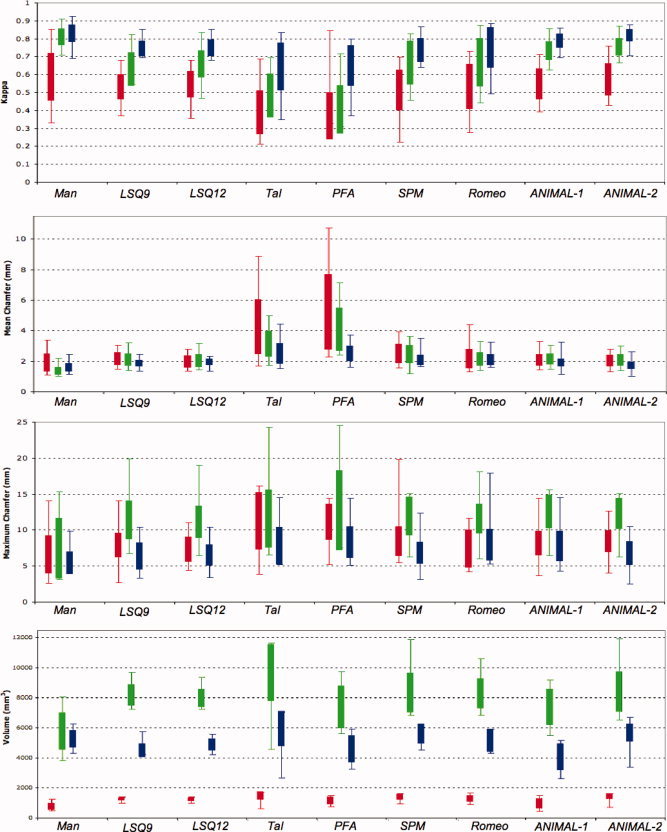
Summary of results from all metrics. From top to bottom: kappa, mean chamfer distance, maximum chamfer distance, and volume results for all methods tested for the globus pallidus (red), striatum (green), and thalamus (blue). Extents of each box represent the standard deviation and error bars represent the range of the data. [Color figure can be viewed in the online issue, which is available at www.interscience.wiley.com.]

The repeated measures ANOVA showed significant differences between the eight techniques tested (F = 13.12, DF = 8, P < 0.0001). The results for the globus pallidus show that the raters (κ_man = 0.587) and both ANIMAL‐based techniques perform statistically better than all other registration techniques tested for atlas‐to‐patient warping (κ_A1 = 0.547, κ_A2 = 0.573). The remaining nonlinear techniques (κ_SPM = 0.513, κ_ROM = 0.532) and the linear techniques (κ_LSQ9 = 0.530, κ_LSQ12 = 0.545) show statistically similar results and have mean kappas lower than the techniques in group A. The piece‐wise linear techniques show the lowest kappa values (κ_TAL = 0.389, κ_SPM = 0.369).

The ANOVA reveals significant differences between the methods tested for the striatum (F = 19.34, DF = 8, P < 0.0001). Results of the post‐hoc analysis demonstrate that the manual raters (κ_man = 0.809) perform statistically better than all other methods. Both ANIMAL‐based techniques perform better than the remaining registration methods and are the only two techniques to have kappas over 0.7 (κ_A1 = 0.732, κ_A2 = 0.754). The linear (κ_LSQ9 = 0.630, κ_LSQ12 = 0.658) and remaining nonlinear (κ_SPM = 0.665, κ_ROM = 0.668) techniques make up the next group, but all fail to reach kappas over 0.7. The piece‐wise linear techniques perform statistically worse than all other techniques (κ_TAL = 0.482, κ_PFA = 0.404).

Kappa results for the thalamus show significant differences between methods (F = 9.56, DF = 8, and P < 0.0001). The post‐hoc analysis shows no significant differences between manual raters (κ_man = 0.829) and ANIMAL‐2 (κ_A2 = 0.818) form group A, however there are no statistical difference between ANIMAL‐1 (κ_A1 = 0.787) and ANIMAL‐2. Once again the remaining nonlinear (κ_SPM = 0.736, κ_ROM = 0.749) and linear techniques (κ_LSQ9 = 0.745, κ_LSQ12 = 0.748) make up the next group, followed by the piece‐wise linear techniques (κ_TAL = 0.643, κ_PFA = 0.649). Only the piece‐wise linear techniques do not achieve the threshold of 0.7.

Mean chamfer distance

The results for the mean distances for each structure and post‐hoc Tukey Kramer HSD are shown in Table IX and a graphical representation is given in the second panel of Figure 5.

Table IX.

Result from post‐hoc Tukey Kramer HSD test for mean chamfer distance (μ) values from raters and all warping techniques for all test structures

	Globus pallidus		Striatum		Thalamus
Method	Groups	Mean ± SD (range)	Groups	Mean ± SD (range)	Groups	Mean ± SD (range)
Manual Raters	A	1.87 ± 0.60 (1.11–3.38)	A	1.34 ± 0.25 (1.00–2.16)	A	1.55 ± 0.28 (1.14–2.44)
LSQ9	A, B	2.10 ± 0.42 (1.46–3.04)	B	2.11 ± 0.40 (1.37–3.19)	B, C	1.82 ± 0.21 (1.34–2.45)
LSQ12	A	1.93 ± 0.40 (1.37–2.80)	B	2.04 ± 0.43 (1.38–3.11)	C	1.91 ± 0.22 (1.34–2.33)
Talairach	C	4.17 ± 1.80 (1.70–8.89)	D	3.13 ± 0.86 (1.69–4.93)	E	2.44 ± 0.68 (1.51–4.44)
PFA	D	5.13 ± 2.47 (2.30–10.73)	E	4.09 ± 1.41 (2.34–7.06)	E	2.45 ± 0.50 (1.61–3.72)
SPM	B	2.45 ± 0.64 (1.55–3.93)	C	2.44 ± 0.60 (1.14–3.60)	D	2.05 ± 0.34 (1.63–3.52)
Romeo	A, B	2.10 ± 0.64 (1.29–4.39)	B, C	2.14 ± 0.45 (1.37–3.27)	D	2.06 ± 0.35 (1.62–3.25)
ANIMAL‐1	A, B	2.03 ± 0.38 (1.43–3.28)	B	2.12 ± 0.36 (1.43–3.01)	B, C	1.85 ± 0.25 (1.13–3.25)
ANIMAL‐2	A, B	2.00 ± 0.37 (1.31–2.81)	B	2.07 ± 0.37 (1.37–2.96)	A, B	1.68 ± 0.24 (1.01–2.64)

Techniques are grouped based on the result of Tukey Kramer HSD post‐hoc analysis (P < 0.05). The mean, minimum, maximum, and standard deviations of the mean chamfer distance are also provided. All distances are provided in millimeters.

ANOVA results for the globus pallidus show significant differences between methods (F = 18.03, DF = 8, P < 0.0001). The manual raters have mean results closest to zero (μ_man = 1.87 mm). The results from the post‐hoc Tukey‐Kramer HSD test show no significant differences between Romeo (μ_ROM = 2.10 mm), the ANIMAL‐based techniques (μ_A1 = 2.03 mm, μ_A2 = 2.00 mm), the linear techniques (μ_LSQ9 = 2.10 mm, μ_LSQ12 = 1.93 mm), and the manual raters. However, no significant differences were observed between SPM (μ_SPM = 2.45 mm) and LSQ9 and nonlinear techniques. The Talairach (μ_TAL = 4.17 mm) and PFA (μ_PFA = 5.13 mm) techniques perform significantly worse than all other techniques and have significantly different results from one another.

Repeated measures ANOVA results for the striatum show significant differences between methods (F = 22.26, DF = 8, P < 0.0001). The manual raters, once again show mean error closest to zero (μ_man = 1.34 mm). No significant differences were observed between Romeo (μ_ROM = 2.14 mm), the ANIMAL‐based techniques (μ_A1 = 2.12 mm, μ_A2 = 2.07 mm) and the linear techniques (μ_LSQ9 = 2.11 mm, μ_LSQ12 = 2.04 mm). However, no significant differences were observed between SPM (μ_SPM = 2.44 mm) and Romeo. Once again, the Talairach (μ_TAL = 3.13 mm) and PFA (μ_PFA = 4.09 mm) techniques perform significantly worse than all other techniques and have significantly different results from one another.

Thalamic ANOVA results demonstrate statistically significant differences (F = 12.56, DF = 8, P < 0.0001). The manual raters demonstrated the mean error with value closest to zero (μ_man = 1.55 mm). The post‐hoc Tukey Kramer HSD demonstrated no significant differences between the manual raters, and ANIMAL‐2 (μ_A2 = 1.68 mm). The LSQ9 (μ_LSQ9 = 1.82 mm) and ANIMAL‐based techniques (μ_A1 = 1.85 mm) also show no significant differences. The linear techniques (μ_LSQ12 = 1.91 mm) formed group C, while SPM (μ_SPM = 2.05 mm), and Romeo (μ_ROM = 2.06 mm) formed group D. The piece‐wise ‐linear techniques formed the group with largest error (μ_TAL = 2.44 mm, μ_PFA = 2.45 mm).

Maximum chamfer distance

The results for the maximum chamfer distances for each structure and post‐hoc Tukey Kramer HSD are shown in Table X and a graphical representation is provided in the third panel of Figure 5.

Table X.

Result from post‐hoc Tukey Kramer HSD test for difference for maximum chamfer distance (M) values from raters and all warping techniques and structures

	Globus pallidus		Striatum		Thalamus
Method	Groups	Mean ± SD (range)	Groups	Mean ± SD (range)	Groups	Mean ± SD (range)
Manual raters	A	6.59 ± 2.68 (2.50–13.91)	A	7.30 ± 5.01 (3.10–15.32)	A	5.33 ± 1.58 (2.43–9.85)
LSQ9	B, C	7.88 ± 1.67 (2.52–13.91)	B	11.15 ± 2.68 (6.75–19.89)	A, B	6.23 ± 1.65 (3.24–10.43)
LSQ12	A, B	7.27 ± 1.74 (4.25–10.92)	B	10.92 ± 2.25 (6.42–18.98)	A, B	6.37 ± 1.45 (3.86–10.38)
Talairach	D	11.21 ± 3.98 (3.65–14.92)	B	11.33 ± 4.01 (6.50–24.32)	C	7.67 ± 2.59 (4.64–14.54)
PFA	D	11.10 ± 2.54 (4.98–14.21)	B	12.47 ± 5.52 (7.50–24.52)	D	8.14 ± 2.20 (4.64–14.40)
SPM	B, C	8.39 ± 2.07 (5.30–19.62)	B	11.67 ± 2.68 (6.24–15.06)	C, D	6.68 ± 1.49 (4.23–12.35)
Romeo	A, B, C	7.39 ± 2.64 (4.03–11.53)	B	11.35 ± 2.05 (6.04–18.08)	C, D	7.77 ± 2.23 (4.44–17.92)
ANIMAL‐1	B, C	8.19 ± 1.70 (3.48–14.29)	B	12.28 ± 2.33 (6.42–15.60)	C, D	7.63 ± 2.10 (3.52–14.48)
ANIMAL‐2	C	8.45 ± 1.52 (3.85–12.51)	B	12.04 ± 2.17 (6.24–15.08)	B, C	6.64 ± 1.69 (2.52–10.46)

Techniques are grouped based on the result of Tukey Kramer HSD post‐hoc analysis (P < 0.05). The mean, minimum, maximum, and standard deviations of the maximum chamfer distance are also provided. All distances are provided in millimeters.

The results from the repeated measures ANOVA show significant differences between all labeling methods (F = 11.28, DF = 8, P < 0.0001) for the globus pallidus. The manual raters show mean error closest to zero (M _man = 6.59 mm). Results from the post‐hoc Tukey Kramer HSD showed no significant differences between the raters, LSQ12 (M _LSQ12 = 7.27 mm), and Romeo (M _ROM = 7.39 mm). A second group showing no significant differences was formed by the linear techniques (M _LSQ9 = 7.88 mm), SPM (M _SPM = 8.39 mm), Romeo, and ANIMAL‐1 (M _A1 = 8.19 mm). Group C was formed by LSQ9, SPM, Romeo, and the ANIMAL‐based techniques (M _A2 = 8.45 mm). The piece‐wise linear techniques (M _TAL = 11.21 mm, M _PFA = 11.10 mm) showed significantly larger errors than all other methods.

The repeated measures ANOVA showed significant differences between all methods used for the data from the striatum (F = 19.29, DF = 8, P < 0.0001). The results of the post‐hoc analysis show that the manual raters (M _man = 7.30 mm) have significantly smaller error values than tested methods. All other warping techniques show no significant differences between results and are listed in here in descending order: LSQ12 (M _LSQ12 = 10.92 mm), LSQ9 (M _LSQ9 = 11.15 mm), Romeo (M _ROM = 11.35 mm), SPM (M _SPM = 11.67 mm), ANIMAL‐2 (M _A2 = 12.04 mm), ANIMAL‐1 (M _A1 = 12.28 mm), and PFA (M _PFA = 12.47 mm).

The repeated measures ANOVA, once again showed differences between all techniques for the thalamus (F = 11.27, DF = 8, P < 0.0001). The manual raters show errors closest to zero (M _man = 5.33 mm). The post‐hoc Tukey Kramer HSD showed that the linear techniques (M _LSQ9 = 6.23 mm, M _LSQ12 = 6.37 mm) had no significant differences with the raters and also formed Group B with ANIMAL‐2 (M _A2 = 6.64 mm). Group C was formed by Talairach (M _TAL = 7.67 mm), SPM (M _SPM = 6.68 mm), Romeo (M _ROM = 7.77 mm), and the ANIMAL‐based (M _A1 = 7.63 mm) techniques. The final group was formed by the PFA (M _PFA = 8.14 mm), SPM, Romeo, and ANIMAL‐1 techniques.

Volume

The results from the analysis of the volume (including results from corresponding post‐hoc analyses) are in Table XI and a graphical representation is given at the bottom of Figure 5.

Table XI.

Result from post‐hoc Tukey Kramer HSD test for volumes (V) from raters and all warping techniques for all test structures

	Globus pallidus		Striatum		Thalamus
Method	Groups	Mean ± SD (range)	Groups	Mean ± SD (range)	Groups	Mean ± SD (range)
Manual Raters	A	710 ± 216 (469–1224)	A	5786 ± 1234 (3719–7918)	B, C	5155 ± 576 (4316–6274)
LSQ9	C, D	1187 ± 110 (998–1393)	B	8194 ± 721 (7105–9543)	A,B, C	4404 ± 440 (4228–5753)
LSQ12	B, C	1157 ± 98 (989–1359)	B	7978 ± 593 (7074–9243)	B, C	4777 ± 364 (4231–5566)
Talairach	D	1406 ± 278 (632–1703)	C	9667 ± 1895 (4386–11 456)	D	5823 ± 1184 (2679–7091)
PFA	B	1090 ± 239 (749–1475)	B	7383 ± 1425 (5437–9581)	A, B	4500 ± 902 (3226–5908)
SPM	B, C	1312 ± 179 (946–1580)	B, C	8338 ± 1306 (6678–11 730)	C	5501 ± 683 (4557–6059)
Romeo	B, C	1210 ± 182 (904–1660)	B, C	8290 ± 1004 (6685–10 455)	B, C	5065 ± 741 (4312–5908)
ANIMAL‐1	B	935 ± 333 (447–1477)	B	7398 ± 1209 (5310–9078)	A	3951 ± 888 (2614–5178)
ANIMAL‐2	B, C	1361 ± 163 (716–1602)	B, C	8414 ± 1343 (6381–11 768)	B	5563 ± 588 (3385–6717)

Techniques are grouped based on the result of Tukey Kramer HSD post‐hoc analysis (P < 0.05). The mean, minimum, maximum, and standard deviations of the volumes are also provided. All distances are provided in cubic millimeters.

The repeated measures ANOVA, showed differences between all techniques for the globus pallidus (F = 11.65, DF = 8, P < 0.0001). The post‐hoc analysis revealed that the average silver standard of the manual raters show a mean volume significantly lower than any of the automated methods (V _man = 710 mm³). The LSQ12 (V _LSQ12 = 1,157 mm³), PFA (V _PFA = 1,090 mm³), and nonlinear techniques (V _SPM = 1,312 mm³, V _ROM = 1,210 mm³, V _A1 = 935 mm³, V _A2 = 1,361 mm³), yield volumes of which are not significantly different from one another. Results from the linear techniques (V _LSQ9 = 1,187 mm³), SPM, Romeo, and ANIMAL‐2 show no significant differences between them. Similarly LSQ9 and Talairach (V _TAL = 1,406 mm³) show no significant differences between them.

The repeated measures ANOVA, revealed differences between all techniques for the striatum (F = 10.95, DF = 8, P < 0.0001). The post‐hoc analysis demonstrated that the average silver standard of the manual raters (V _man = 5,786 mm³) show significantly smaller volumes than the rest of the atlas warping techniques tested. The linear techniques (V _LSQ9 = 8,194 mm³, V _LSQ12 = 7978 mm³), the PFA (V _PFA = 7383 mm³) and the nonlinear techniques (V _SPM = 8338 mm³, V _ROM = 8290 mm³, V _A1 = 7398 mm³, V _A2 = 8,414 mm³) show significantly higher volumes when compared than the manual raters, but show no differences between them. The Talairach technique shows the highest volume (V _TAL = 9,667 mm³) and no differences with SPM, Romeo, and ANIMAL‐2.

The repeated measures ANOVA, once again showed differences between all techniques for the thalamus (F = 11.15, DF = 8, P < 0.0001). The ANIMAL‐1 (V _A1 = 3951 mm³) technique showed the lowest volume and the post‐hoc analysis showed no differences with the PFA (V _PFA = 4,500 mm³) and LSQ9 (V _LSQ9 = 4,404 mm³). No significant differences were observed between the manual raters (V _man = 5,155 mm³), LSQ9, LSQ12 (V _LSQ12 = 4,777 mm³), PFA (V _PFA = 4,500 mm³), Romeo (V _ROM = 5,065 mm³), and ANIMAL‐2 (V _A1 = 5,563 mm³). SPM (V _SPM = 5,501 mm³) has higher volumes and has no differences with the manual raters, LSQ9, LSQ12, PFA, and Romeo. Talairach (V _TAL = 5,823 mm³) shows the highest volume and is significantly different than all other techniques.

DISCUSSION

Summary

This paper presents a comparison of eight different registration techniques in order to evaluate their accuracy, precision, and consistency for atlas‐to‐patient warping. The digital atlas used was developed in our group using a segmented set of serial histological data [Chakravarty et al., 2006a]. The reconstructed atlas was nonlinearly warped to a high signal‐ and contrast‐to‐noise ratio template [Holmes et al., 1998].

Two linear techniques based on the least‐squares optimization of the cross‐correlation objective function [Collins et al., 1994] were used to estimate 9‐parameter (3 translations, rotations, and scales) and a 12‐parameter (3 translations, rotations, scales, and shears) transformations.

Two piece‐wise linear techniques requiring the manual identification of homologous landmarks on both the template and the patient imaging volumes were also evaluated. The first is the well‐known Talairach transformation [Talairach and Tournoux, 1988] which separates both the template and the patient MRI volume into 12 different subvolumes, and estimates a unique 9‐parameter linear transformation for each of these sections. The second is the PFA technique (used in [Nowinski et al., 2003] in the development of a probabilistic functional atlas), which estimates a unique nine‐parameter transformation per hemisphere, based on subcortical landmarks.

Nonlinear transformations were estimated using four different methods. The first is from the well known SPM package [Friston et al., 1995a, b] and estimates a transformation based on the sixth order expansion of a set of smoothly varying spatial basis functions (discrete cosine transform) optimized using a least squares procedure. The second nonlinear technique (the Romeo algorithm) was developed by Hellier et al. [ 2001] and uses the optical flow hypothesis to estimate a nonlinear transformation through minimization of a luminance equation using an iterative hierarchal registration strategy. The last two techniques are based on the ANIMAL algorithm developed by Collins and coworkers [Collins and Evans, 1997; Collins et al., 1995] and optimized by Robbins et al. [ 2004]. The first uses the standard implementation of ANIMAL used at the Montréal Neurological institute and was called ANIMAL‐1 in this paper. This technique uses a hierarchical registration strategy to maximize the similarity between the template and patient MRI volumes. The final transformation was defined on a set of nodes spaced 2 mm apart. The second ANIMAL‐based technique (called ANIMAL‐2 in this paper) estimates a transformation using only a cropped region of the template volume focused only on the thalamus and the basal ganglia. This permitted the estimation of a final nonlinear transformation on set of nodes spaced 1 mm apart.

All atlas‐warping techniques were validated against manual segmentations of the globus pallidus, striatum, and thalamus. In the absence of an anatomical “gold standard” a series of “silver standards” were created from the manual labels in a leave‐one‐out fashion, where a single rater's labels are compared to a silver standard developed through the agreement of other labels. Four metrics were used to evaluate the atlas warping techniques. The first was the kappa which assesses the overlap between two sets of labels. The second is the maximum of the chamfer distance [Borgefors, 1984] between the surfaces of two sets of labels and is an approximation of the Hausdorff distance. The third uses the mean distance between the surfaces of two label volumes. The final is the total volume for each structure.

On the Use of a Silver Standard

One of the main novelties of this study resides in the use and derivation of a silver standard from manual raters for the comparison of different registration techniques used for atlas warping. Despite the variability of the manual raters definitions, each rater used is known to have an accurate definition of the structures tested and the method used in this study shows that the raters can effectively provide an upper limit for the accuracy of anatomical labeling.

Work by Warfield et al. [ 2004] has addressed this issue by developing an expectation maximization algorithm that estimates an optimal segmentation from the different methods being evaluated. Using this technique, each method can then be weighted depending upon its estimated performance level with respect to the other methods being tested. The specificity and sensitivity parameters used in STAPLE could add valuable information to the evaluation of the data presented in this paper. Furthermore, the probabilistic ground truth of the manual rater data generated by STAPLE could also be used for evaluation instead of the discrete silver standard generated through consensus used in the work presented here.

Quality of the Silver Standard

To estimate the variability between the labels provided by each of the raters, all labels from manual rater were assessed using the metrics that were described in the Methods section. All results show significant variability for all raters across all metrics (except for the maximum chamfer distance test in the striatum). Statistically, tests revealed that while each manual rater may have a different definition of the subcortical structures that were labeled, none could be considered outliers from the rest of the raters. However the variability of the results demonstrate the difficulty in obtaining a consistent estimate for the location of different anatomical structures. This underscores the importance of using the five different silver standard estimates of the anatomy for each anatomical structure tested in these experiments. This variability in manual segmentation also underscores the need for an automated, objective, and robust technique to identify the basal ganglia and thalamus in patients for surgical planning for movement disorders. Better identification of the anatomy should lead to better identification of the functional targets, and thus better clinical results after surgery.

It is important to note that the lack of a gold standard limits our ability to evaluate the segmentation procedures. Essentially, none of the automatic techniques can agree more with the silver standard that the manual raters agree with each other. Thus, the mean kappa of the manual raters acts as a ceiling for the kappa values associated with the automatic techniques.

Overlap of Structures

The kappa metric was used to compare the agreement between structures manually defined in the silver standards and those defined by the 8 different atlas‐customization techniques. While the kappa metric is often used for such comparisons, it is not without problems. First, if one assumes that the difference between label sets will occur at structure borders, then the kappa will discriminate against smaller structures. Therefore, the lower mean kappas found for the globus pallidus were expected. Second, kappa depends on the surface to volume ratio of the structure. For example, the striatum (containing the putamen, nucleus accumbens and caudate) has roughly the same volume as the thalamus, but has perhaps twice the surface area. This explains the consistently higher kappa values for the thalamus. Finally, the atlas was defined using a set of high‐resolution and high‐contrast histological data and contains certain structural details that could not be identified by the raters at the posterior pallidum and striatum, thus negatively biasing the kappa values for the striatum and globus pallidus.

The results demonstrate a similar pattern over all structures (Table VIII). The consistently lower kappa values for the Talairach and PFA techniques may be due to errors associated with manual landmark identification and the limited degrees of freedom offered by the PFA technique. One could also expect the piece‐wise linear techniques to outperform the linear techniques; however this is not the case here. We hypothesize that this may be due to landmark placement issues inherent in algorithms requiring manual feature identification. Furthermore, the transformation optimization strategy employed in the fitting of the template volume to the patient volume may serve as an advantage when compared to the limited features of the piece‐wise linear techniques.

Surprisingly, the LSQ9, LSQ12, SPM and Romeo techniques yield similar results. With their additional degrees of warping freedom, one would expect that SPM and Romeo techniques would yield better results compared to the linear matching methods. This also contradicts our hypothesis as all nonlinear registration algorithms will not offer better identification of subcortical structures when compared to linear techniques. Further, this suggests that the choice of nonlinear algorithm is crucial for automated identification of subcortical targets. However, given the number of patients labeled and the variability of the kappa values between patients, there may not be sufficient statistical power to tease out a separation between these techniques. In particular, Romeo was designed using a hypothesis that the luminescence between source and target volumes will be similar. The acquisition limitations inherent to data acquired with the stereotactic headframe limits grey/white matter contrast, thus the luminescence hypothesis may not be valid when matching this data to a high‐contrast, high‐resolution template. Romeo may benefit from the usage of a single MRI template that is selected from a database of population‐ and acquisition‐specific MRI‐volumes [D'Haese et al., 2005b]. For an application such as this the correlation coefficient may be a more robust similarity criterion. This interpretation is supported by the results from both ANIMAL‐based techniques as they consistently yielded the best kappa values. Finally, for the globus pallidus and thalamus, the ANIMAL‐2 technique yielded kappas that were not different from the manual raters, indicating that it performed on par with the expert anatomists for these two structures in this set of patients.

Distance Metrics, Volumes, and the Bias of the Atlas

While the kappa value gives an idea of how well the label sets overlap, its value cannot be easily translated to a quantitative measure of structure mismatch. For this reason we computed the mean chamfer distance metric, μ, to judge how well the atlas customization procedures could identify the structure borders on each patients' MRI. To place the automatic procedures in context, the 3D mean chamfer distances were 1.34 mm, 1.55 mm and 1.87 mm for the manually identified striatum, thalamus and globus pallidus, respectively. Given the discrete nature of the voxel labels, this means that on average, each of the manual raters were within approximately a single voxel of the sliver standard in any of the transverse, coronal or sagittal planes.

The pattern of mean chamfer distance results (Table IX) for the automatic procedures is not as clear as that seen for the kappa metric. The Talairach and PFA techniques consistently have the largest mean mismatch over the three structures (2.44‐5.13 mm). This may be due to the limitations of these techniques discussed above. Surprisingly, the LSQ12 technique marginally outperforms all other automated techniques evaluated for the globus pallidus and the striatum. An additional surprise is SPM's poor performance on these two structures. Of the remaining automated techniques (LSQ9, LSQ12, Romeo, and ANIMAL‐1, ANIMAL‐2), none is clearly superior based on the pallidal and striatal results, however ANIMAL‐2 shows nearly identical values to LSQ12 for these structures. The main improvement of the ANIMAL‐based techniques is in the thalamus, where ANIMAL‐2 shows lowest values.

The maximum chamfer distance (Table X) results are heavily biased by resolution differences between the MRI data and the atlas. The high‐resolution and contrast of the initial histological data used to develop the atlas heavily biases these results. In particular small substructures at the tails of the globus pallidus and striatum can be resolved on the histological data and not on the pre‐operative MRI data. The striatal results are a reflection of this difference as all warping methods show no significant differences, but have approximately 4–5 mm more error than that of the manual raters. These differences explain the variability in the results for the globus pallidus and the thalamus. The results demonstrate that the nonlinear techniques are prone to outliers in the thalamus and in the globus pallidus. Due to the nature of the pre‐operative acquisition, local fitting at the borders of these structures and the internal capsule is compromised. This may explain why in the thalamus, the groups formed by the raters and linear methods yield the lowest error. The poor performance of the piece‐wise linear techniques may again be linked to the manually selected landmarks required for these techniques.

The significant differences between the volume (Table XI) of the structures defined by the atlas and the manual raters for both the globus pallidus and the striatum may also be due to the difference in spatial resolution of the atlas and the MR data (as mentioned above). Results from the Talairach techniques suggest that it consistently over estimates the volume of each structure, while the PFA technique consistently provides volumes that are closest to the manual raters. The choice of landmarks used for transformation estimation may be the reason for these differences. The Talairach technique uses cortical landmarks, while the PFA technique uses only subcortical landmarks. Thus the PFA may actually account for subcortical atrophy in these structures better than other the Talairach technique, however it may be limited in accuracy (as seen above). However, no other technique yields a consistently larger (or smaller) volume across all structures, thus it is difficult to draw further conclusions from this test.

CONCLUSIONS AND FUTURE WORK

In this paper eight different techniques (two linear, two piece‐wise linear, and four nonlinear) were compared against manual raters for atlas‐to‐patient warping. It was shown that the ANIMAL‐2 algorithm (estimating a final transformation of a set of nodes with 1 mm spacing) gave the best results using the kappa metric and was consistently amongst the lowest in the mean chamfer distance test. These two tests also showed that the two piece‐wise linear techniques tested (PFA and Talairach) performed significantly worse when compared to the other techniques.

Future work will involve testing with other nonlinear registration algorithms and intra‐operative data used for target localization and post‐operative data. Further prospective and retrospective studies will be performed on additional patient data to determine the clinical efficacy of this atlas for the localization of subcortical surgical targets.

REFERENCES

- Atkinson J,Collins DL,Bertrand G,Peters TM,Pike B,Sadikot AF 2002. Optimal location of thalamotomy lesions for tremor associated with Parkinson's disease: a probabilistic analysis based on postoperative magnetic resonance imaging and integrated digital atlas. J Neurosurg 96: 854–866. [DOI] [PubMed] [Google Scholar]
- Bardinet E,Dormont D,Malandain G,Bhattacharjee M,Pidoux B,Saleh C,Cornu P,Ayache N,Agid Y,Yelnik J ( 2005): Retrospective cross‐evaluation of a histological and deformable 3D atlas of the basal ganglia on series on Parkinsonian patients treated by deep brain stimulation In: Seventh International Conference on Medical Image Computing and Computer Assisted Intervention MICCAI 2005, Palm Springs, USA. Lecture Notes in Computer Science 3750, vol. 2 Springer; pp 385–393. [DOI] [PubMed] [Google Scholar]
- Behrens TEJ,Johansen‐Berg H,Woolrich MW,Smith SM,Wheeler‐Kingshot CAM,Boulby PA,Barker GJ,Sillery EL,Sheehan K,Ciccarelli O,Thompson AJ,Brady JM,Matthews PM ( 2003): Non‐invasive mapping of connections between human thalamus and cortex using diffusion imaging. Nat Neurosci 6: 750–757. [DOI] [PubMed] [Google Scholar]
- Bejjani BP,Dormont D,Pidoux B,Yelnik J,Damier P,Arnulf I,Bonnet AM,Marsault C,Agid Y,Philippon J,Cornu P ( 2000): Bilateral subthalamic stimulation for Parkinson's disease by using three dimensional stereotactic magnetic resonance imaging and electrophysiological guidance. J Neurosurg 92: 615–625. [DOI] [PubMed] [Google Scholar]
- Benabid AL,Koudsié A,Benazzouz A,Le Bas JF,Pollak P ( 2002): Imaging of subthalamic nucleus and ventralis intermedius of the thalamus. Movement Disorders 17: S123–S129. [DOI] [PubMed] [Google Scholar]
- Bertrand G ( 1982): Stereotaxy of the Human Brain. Anatomical, Physiological and Clinical Applications, 2nd ed Georg Thieme Verlag; Chapters in Computers in Stereotaxic Surgery. [Google Scholar]
- Bertrand G,Olivier A,Thompson CJ ( 1973): The computerized brain atlas: Its use in stereotaxic surgery. Trans Am Neurol Assoc 98: 233–237. [PubMed] [Google Scholar]
- Bertrand G,Olivier A,Thompson CJ ( 1974): Computer display of stereotaxic brain maps and probe tracts. Acta Neurochirurgica 21( Suppl): 235–243. [DOI] [PubMed] [Google Scholar]
- Borgefors G ( 1984): Distance transformations in arbitrary dimensions. Comput Vision Graphics Image Process 27: 321–345. [Google Scholar]
- Chakravarty MM,Bertrand G,Descoteaux M,Sadikot AF,Collins DL ( 2003): The creation of a brain atlas for image guided neurosurgery In: Fifth International Conference on Medical Image Computing and Computer Assisted Intervention MICCAI 2003, Montréal, Canada. Lecture Notes in Computer Science 2879, vol. 1 Springer; pp 343–350. [Google Scholar]
- Chakravarty MM,Sadikot AF,Germann J,Bertrand G,Collins DL ( 2005): Anatomical and electrophysiological validation of an atlas for neurosurgical planning In: Seventh International Conference on Medical Image Computing and Computer Assisted Intervention MICCAI 2005, Palm Springs, USA. Lecture Notes in Computer Science 3750, vol. 2 Springer; pp 394–401. [DOI] [PubMed] [Google Scholar]
- Chakravarty MM,Bertrand G,Hodge CP,Sadikot AF,Collins DL ( 2006a): The creation of a brain atlas for image guided neurosurgery using serial histological data. NeuroImage 30: 359–376. [DOI] [PubMed] [Google Scholar]
- Chakravarty MM,Sadikot AF,Mongia S,Bertrand G,Collins DL ( 2006b): Towards a multi‐modal atlas for neurosurgical planning In: Eighth International Conference on Medical Image Computation and Computer Assisted Intervention MICCAI 2006, Copenhagen, Denmark. Lecture Notes in Computer Science 4191, Vol. 2 Springer; pp 389–396. [DOI] [PubMed] [Google Scholar]
- Chakravarty MM,Sadikot AF,Germann J,Bertrand G,Collins DL ( 2008a): Towards a validation of atlas warping techniques. Med Image Anal 12: 713–726. [DOI] [PubMed] [Google Scholar]
- Chakravarty MM,Rosa‐Neto P,Broadbent S,Evans AC,Collins DL ( 2008b): Development of fMRI techniques for planning in functional neurosurgery for Parkinson's disease. In: IEEE International Symposium on Biomedical Imaging ISBI 2008, Paris, France. pp 1259–1262.
- Christensen GE,Johnson HJ ( 2001): Consistent image registration. IEEE Trans Med Imaging 20: 568–582. [DOI] [PubMed] [Google Scholar]
- Cohn MC,Hudgins PA,Sheppard SK,Starr PA,Bakay RAE ( 1998): Pre‐ and postoperative evaluation of stereotactic pallidotomy. Am J Neuroradiol 19: 1075–1080. [PMC free article] [PubMed] [Google Scholar]
- Collins DL,Evans AC ( 1997): ANIMAL: Validation and application of nonlinear registration‐based segmentation. Int J Pattern Recog Artif Intell 11: 1271–1294. [Google Scholar]
- Collins DL,Holmes CJ,Peters T,Evans AC ( 1995): Automatic 3‐D model based neuroanatomical segmentation. Hum Brain Mapp 3: 190–208. [Google Scholar]
- Collins DL,Neelin P,Peters TM,Evans AC ( 1994): Automatic 3D intersubject registration of MR volumetric data in standardized Talairach Space. J Comput Assisted Tomogr 18: 192–205. [PubMed] [Google Scholar]
- Deoni SCL,Peters TM,Rutt BK ( 2005): High resolution T1 and T2 mapping of the brain in clinically acceptable time with DESPOT1 and DESPOT2. Magn Reson Med 53: 237–241. [DOI] [PubMed] [Google Scholar]
- D'Haese PF,Pallavaram S,Niermann K,Spooner J,Kao C,Konrad PE,Dawant BM ( 2005a): Automatic selection of dbs target points using multiple electrophysiological atlases In: Seventh International Conference on Medical Image Computing and Computer Assisted Intervention MICCAI 2005, Palm Springs, USA. Lecture Notes in Computer Science 3750, vol. 2 Springer; pp 427–434. [DOI] [PubMed] [Google Scholar]
- D'Haese PF,Cetinkaya E,Konrad PE,Kao C,Dawant BM ( 2005b): Computer‐aided placement of deep brain stimulators: from planning to intraoperative guidance. IEEE Tran Med Imaging 24: 1469–1478. [DOI] [PubMed] [Google Scholar]
- Duda RO,Hart PE,Stork DG ( 2000): Pattern Classification, 2nd ed New York: John Wiley. [Google Scholar]
- Duval C,Strafella AP,Sadikot AF ( 2005): The impact of ventrolateral thalamotomy on high‐frequency components of tremor. Clin Neurophysiol 116: 1391–1399. [DOI] [PubMed] [Google Scholar]
- Eskandar EN,Cosgrove RG,Shinobu LA ( 2001): Surgical treatment of parkinson disease. J Am Med 286: 3056–3059. [DOI] [PubMed] [Google Scholar]
- Finnis KW,Starreveld YP,Parrent AG,Sadikot AF,Peters TM ( 2003): Three‐dimensional database of subcortical electrophysiology for image‐guided stereotactic functional neurosurgery. IEEE Trans Med Imaging 22: 93–104. [DOI] [PubMed] [Google Scholar]
- Friston KJ,Ashburner CD,Frith CD,Poline J‐B,Heather JD,Frackowiak RSJ ( 1995a): Spatial registration and normalization of images. Hum Brain Mapp 3: 165–189. [Google Scholar]
- Friston KJ,Holmes AP,Worsley KJ,Poline J‐B,Frith CD,Frackowiak RSJ ( 1995b): Statistical parametric maps in functional imaging: A general linear approach. Hum Brain Mapp 2: 189–210. [Google Scholar]
- Ganser KA,Dickhaus H,Metzner R,Wirtz CR ( 2004): A deformable digital brain atlas system according to Talairach and Tournoux. Med Image Anal 8: 3–22. [DOI] [PubMed] [Google Scholar]
- Gerig G,Jomier M,Chakos M ( 1998): Valmet: A new validation tool for assessing and improving 3D object segmentation In: Niessen WM, Viergever A, editors. Fourth International Conference on Medical Image Computing and Computer‐Assisted Intervention, MICCAI 2001, Utrecht, The Netherlands. Lecture Notes in Computer Science, vol. 2208 Springer; pp 516–523. [Google Scholar]
- Gloor P ( 1997): The Temporal Lobe and the Limbic System. New York: Oxford University Press. [Google Scholar]
- Gross RE,Lombardi WJ,Lang AE,Duff J,Hutchison WD,Saint‐Cyr JA,Tasker RR,Lozano AM ( 1999): Relationship of lesion location to clinical outcome following microelectrode‐guided pallidotomy for Parkinson's disease. Brain 122: 405–416. [DOI] [PubMed] [Google Scholar]
- Guo T,Finnis KW,Parrent AG,Peters TM ( 2005): Development and Application of functional databases for planning deep‐brain neurosurgical procedures In: Seventh International Conference on Medical Image Computing and Computer Assisted Intervention MICCAI 2005, Palm Springs, USA. Lecture Notes in Computer Science 3750, vol. 1 Springer; pp 835–842. [DOI] [PubMed] [Google Scholar]
- Hellier P,Barillot C,Mémin E,Pérez P ( 2001): Hierarchical estimation of a dense deformation field for 3D robust registration. IEEE Trans Med Imaging 20: 388–402. [DOI] [PubMed] [Google Scholar]
- Hellier P,Barillot C,Corouge I,Gibaud B,LeGoualher G,Collins DL,Evans AC,Malandain G,Ayache N,Christensen GE,Johnson HJ ( 2003): Restrospective evaluation of intersubject brain registration. IEEE Trans Med Imaging 22: 1120–1130. [DOI] [PubMed] [Google Scholar]
- Hirai T,Jones EG ( 1989): A new parcellation of the human thalamus on the basis of histochemical staining. Brain Res Brain Res Rev 14: 1–34. [DOI] [PubMed] [Google Scholar]
- Holmes CJ,Hoge R,Collins L,Woods R,Toga AW,Evans AC ( 1998): Enhancement of MR images using registration for signal averaging. J Comput Assisted Tomogr 22: 324–333. [DOI] [PubMed] [Google Scholar]
- Horn BPK,Schunck BG ( 1981): Determining optical flow. Artif Intell 17: 185–203. [Google Scholar]
- Jannin P,Grova C,Maurer CR Jr ( 2006): Model for defining and reporting reference‐based validation protocols in medical image processing. Int J Comput Assisted Radiol Surg 1: 63–73. [Google Scholar]
- Johansen‐Berg H,Behrens TEJ,Sillery E,Ciccarelli O,Thompson AJ,Smith SM,Matthews PM ( 2005): Functional‐anatomical validation and individual variation of diffusion tractography‐based segmentation of the human thalamus. Cerebral Cortex 15: 31–39. [DOI] [PubMed] [Google Scholar]
- Krause M,Fogel W,Heck A,Hacke W,Bonsanto M,Trenkwalder C,Tronnier V ( 2001): Deep brain stimulation for the treatment of Parkinson's disease: subthalamic nucleus versus globus pallidus internus. J Neurol Neurosurg Psychiatry 70: 464–470. [DOI] [PMC free article] [PubMed] [Google Scholar]
- Lenz FA,Normand SL,Kwan HC,Andrews D,Rowland LH,Jones MW,Seike M,Lin YC,Tasker RR,Dostrovsky JO,Lenz YE ( 1995): Statistical prediction of the optimal site for thalamotomy in parkinsonian tremor. Movement Disorders 10: 318–328. [DOI] [PubMed] [Google Scholar]
- Lombardi WJ,Gross RE,Trepanier LL,Lang AE,Lozano AM,Saint‐Cyr JA ( 2000): Relationship of lesion location to cognitive outcome following microelectrode‐guided pallidotomy for Parkinson's disease: Support for the existence of cognitive circuits in the human pallidum. Brain 123: 746–758. [DOI] [PubMed] [Google Scholar]
- Maes F,Collignon A,Vandermeulen D,Marchal G,Suetens P ( 1997): Multimodality image registration by maximization of mutual information. IEEE Trans Med Imaging 16: 187–198. [DOI] [PubMed] [Google Scholar]
- Neelin P,MacDonald D,Collins DL,Evans AC ( 1998): The MINC file Format, from bytes to brains. In: Evans AC, editor. The 4th International Conference on Functional Mapping of the Human Brain, Montréal, Canada. Organization for Human Brain Mapping. p 786.
- Nowinski WL,Fang A,Nguyen BT,Raphel JK,Jagannathan L,Raghavan R,Bryan NR,Miller GA ( 1997): Multiple brain atlas database and atlas based neuroimaging system. Comput Aided Surg 2: 42–66. [DOI] [PubMed] [Google Scholar]
- Nowinski WL,Yang GL,Yeo TT ( 2000): Computer aided stereotactic functional neurosurgery enhanced by the use of the multiple brain atlas database. IEEE Trans Med Imaging 19: 62–69. [DOI] [PubMed] [Google Scholar]
- Nowinski WL,Belov D,Benabid AL ( 2003): An algorithm for rapid calculation of a probabilistic functional atlas of subcortical structures from electrophyisiological data collected during functional neurosurgical procedures. NeuroImage, 18: 143–155. [DOI] [PubMed] [Google Scholar]
- Ono M,Kubik S,Abernathy CD ( 1990): Atlas of the Cerebral Sulci. Stuttgart: Georg Thieme Verlag; Thieme Medical Publishers. [Google Scholar]
- Otsuki T,Jokura H,Takahashi K,Ishikawa S,Yoshimoto T,Kimura M,Yoshida R,Miyazawa T ( 1994): Sterotactic gamma‐thalamotomy with a computerized brain atlas: Technical case report. Neurosurgery 35: 764–768. [DOI] [PubMed] [Google Scholar]
- Robbins S,Evans AC,Collins DL,Whitesides S ( 2004): Tuning and comparing spatial normalization methods. Med Image Anal 8: 311–323. [DOI] [PubMed] [Google Scholar]
- Rohde GK,Aldroubi A,Dawant BM ( 2003): The adaptive bases algorithm for intensity based non‐rigid image registration. IEEE Trans Med Imaging 22: 1470–1479. [DOI] [PubMed] [Google Scholar]
- Rueckert D,Sonoda LI,Hayes C,Hill DLG,Leach MO,Hawkes DJ ( 1999): Nonrigid registration using free‐form deformations: Application to breast MR images. IEEE Trans Med Imag 18: 712–721. [DOI] [PubMed] [Google Scholar]
- Sanchez Castro FJ,Pollo C,Meuli R,Maeder P,Bach Cuadra M,Cuisenaire O,Villemure JG,Thiran JP ( 2005): Cross validation of experts versus registration method for target localization in deep brain stimulation In: Seventh International Conference on Medical Image Computing and Computer Assisted Intervention MICCAI 2005, Palm Springs, USA. Lecture Notes in Computer Science 3750, Vol. 1 Springer; pp 417–424. [DOI] [PubMed] [Google Scholar]
- Sanchez Castro FJ,Pollo C,Villemure JG,Thiran JP ( 2006): Validation of experts versus atlas‐based and automatic registration methods for subthalamic nucleus targeting on MRI. Int J Comput Assisted Radiol Surg 1: 5–12. [Google Scholar]
- Schaltenbrand G,Bailey W ( 1959): Atlas of Stereotaxy of the Human Brain. Stuttgart: Georg Thieme Verlag. [Google Scholar]
- Schaltenbrand G,Wahren W ( 1977): Atlas for Stereotaxy of the Human Brain. Stuttgart: Georg Thieme Verlag. [Google Scholar]
- Smith SM,Jenkinson M,Woolrich MW,Beckmann CF,Behrens TEJ,Johansen‐Berg H,Bannister PR,De Luca M,Drobnjak I,Flitney DE,Niazy R,Saunders J,Vickers J,Zhang Y,De Stefano N,Brady JM,Matthews P ( 2004): Advances in functional and structural MR image analysis and implementation as FSL. NeuroImage 23(S2): 208–219. [DOI] [PubMed] [Google Scholar]
- St‐Jean P,Sadikot AF,Collins L,Clonda D,Kasrai R,Evans AC,Peters TM ( 1998): Automated atlas integration and interactive three‐dimensional visualization tools for planning and guidance in functional neurosurgery. IEEE Trans Med Imaging 17: 672–680. [DOI] [PubMed] [Google Scholar]
- Starr PA,Vitek JL,DeLong M,Bakay RA ( 1999): Magnetic resonance imaging‐based stereotactic localization of the globus pallidus and subthalamic nucleus. Neurosurgery 44: 303–314. [DOI] [PubMed] [Google Scholar]
- Talairach J,Tournoux P ( 1988): Co‐Planar Stereotaxic Atlas of the Human Brain. Stuttgart: Georg Thieme Verlag. [Google Scholar]
- Thirion J‐P ( 1998): Image matching as a diffusion process: an analogy with Maxwell's demons. Med Image Anal 2: 243–260. [DOI] [PubMed] [Google Scholar]
- Warfield SK,Zou KH,Wells WM ( 2004): Simultaneous truth and performance level estimation (STAPLE): an algorithm for the validation of image segmentation. IEEE Trans Med Imaging 23: 903–921. [DOI] [PMC free article] [PubMed] [Google Scholar]
- Woods RP,Grafton ST,Holmes CJ,Cherry SR,Mazziotta JC ( 1998a): Automated image registration. I. General methods and intrasubject, intramodality validation. J Comput Assisted Tomogr 22: 139–152. [DOI] [PubMed] [Google Scholar]
- Woods RP,Grafton ST,Watson JDG,Sicotte NL,Mazziotta JC ( 1998b): Automated image registration. II. Intersubject validation of linear and nonlinear models. J Comput Assisted Tomogr 22: 153–165. [DOI] [PubMed] [Google Scholar]
- Xu M,Nowinski WL ( 2001): Talairach–Tournoux brain atlas registration using a metalforming principle‐based finite element method. Med Image Anal 5: 271–279. [DOI] [PubMed] [Google Scholar]
- Yelnik J,Bardinet E,Dormont D,Malandain G,Ourselin S,Tandé D,Karachi C,Ayache N,Cornu P,Agid Y ( 2007): A three dimensional, histological and deformable atlas of the human basal ganglia. I. Atlas construction based on immuno histochemical and MRI data. NeuroImage 34: 618–638. [DOI] [PubMed] [Google Scholar]