

Abstract
Identifying directional influences in anatomical and functional circuits presents one of the greatest challenges for understanding neural computations in the brain. Granger causality mapping (GCM) derived from vector autoregressive models of data has been employed for this purpose, revealing complex temporal and spatial dynamics underlying cognitive processes. However, the traditional GCM methods are computationally expensive, as signals from thousands of voxels within selected regions of interest (ROIs) are individually processed, and being based on pairwise Granger causality, they lack the ability to distinguish direct from indirect connectivity among brain regions. In this work a new algorithm called PCA based conditional GCM is proposed to overcome these problems. The algorithm implements the following two procedures: (i) dimensionality reduction in ROIs of interest with principle component analysis (PCA), and (ii) estimation of the direct causal influences in local brain networks, using conditional Granger causality. Our results show that the proposed method achieves greater accuracy in detecting network connectivity than the commonly used pairwise Granger causality method. Furthermore, the use of PCA components in conjunction with conditional GCM greatly reduces the computational cost relative to the use of individual voxel time series. Hum Brain Mapp, 2009. © 2008 Wiley‐Liss, Inc.
Keywords: causality, conditional Granger causality mapping (cGCM), principal component analysis (PCA), fMRI
INTRODUCTION
Functional magnetic resonance imaging (fMRI) plays an important role in the in vivo study of cognitive processing in the human brain. Currently, research in the fMRI field is undergoing a transition from mapping sites of activation towards identifying the connectivity that weaves these sites together into dynamic systems of temporally and spatially interacting neural elements [Goebel et al.,2003; Lee et al.,2003]. Impressive conceptual and methodological progress has been made since the first description of the functional MRI effect [Ogawa and Lee,1990]. In particular, functional integration [Friston,2002] has been proposed as the basis for interpreting changes in the correlation structures between different brain regions. Recently, a Granger causality mapping (GCM) method based on vector autoregressive (VAR) models of fMRI time series [Goebel et al.,2003; Roebroeck et al.,2005; Sato et al.,2006] was used to map effective connectivity in the human brain, promising further insights into the neural mechanisms of cognitive processing by revealing how one brain region might exert influence on another.
Previous neuroimaging studies have shown that multiple brain regions organized in interacting networks are required to perform cognitive tasks [Dagher et al.,1999; Liu et al.,1999; Londei et al.,2007; Owen et al.,1996]. Directional information provided by Granger causality offers the potential for defining the anatomical pathways that underlie neural interactions. As the traditional pairwise Granger causality mapping (pGCM) method cannot clearly distinguish between direct causal influences from one region to another and indirect ones mediated through a third region [Chen et al.,2006; Geweke,1984], it is thus felt that pGCM is not suited for this task, given the extreme anatomical complexity of the human brain. Recent work shows that the conditional Granger causality measure can overcome this problem [Chen et al.,2006]. Direct and indirect causal influences between areas in a neural network and their relative weights could be used to either generate hypothesis regarding the underlying anatomical connectivity or test hypothesis formulated from known anatomical connectivity in a given problem.
Most commonly, fMRI data from individual voxels or from averaging over multiple voxels were directly treated as a vector time series in brain connectivity studies [Goebel et al.,2003; Roebroeck et al.,2005; Sato et al.,2006]. Some of the disadvantages of these methods are: (1) the fitting of the VAR model to individual voxels incurs a large computational cost, and (2) the averaging operation may lose part of the information in the time series. Principal component analysis (PCA) [Jolliffe,1986; Polat and Günes,2007] is ideally suited to identify a substantially smaller group of time series than the number of voxels in a region of interest (ROI) that can still adequately account for its activity. In the current study, PCA is employed to reduce the dimensionality of blood oxygen level dependent (BOLD) data in known ROIs by combining correlated features into a set of new orthogonal variables called principal components (PCs). The PCA representation reduces computational cost, while preserving statistical information.
The PCA based conditional Granger causality mapping (PCA‐cGCM) will be first tested on simulated fMRI data. Comparison with the traditional pGCM and other related approaches is made to illustrate the advantage of the proposed new method. The fMRI data from humans performing an emotional task were then analyzed. In particular, the directional relationship between the right amygdala and other activated brain regions was clarified.
METHODS
Principal Component Analysis
PCA [Jolliffe,1986] is a multivariable statistical analysis technique for data compression and feature extraction. PCA seeks linear combinations of the original variables such that the derived variables capture maximal variance. More specifically, for a given n‐dimensional matrix n × m, where n and m are the number of variables and the number of temporal observations, respectively, the p principal axes (p ≪ n) are orthogonal axes, onto which the retained variance is maximal in the projected space. The PCA describes original data space in a base of eigenvectors. The corresponding eigenvalues account for the energy of the process in the eigenvector directions. It is assumed that most of the information in the observation vectors is contained in the subspace spanned by the first p PCs. Considering data projection restricted to p eigenvectors with the highest eigenvalues, an effective reduction in dimensionality of the original data input space can be achieved with minimal information loss [Soares‐Filho et al.,2001]. Details of calculations used in PCA can be found in Song and Shao [1997]. Reducing the dimensionality of the n dimensional input space by projecting input data onto the reduced number of p directions is an important step that facilitates subsequent Granger causality analysis.
Conditional Granger Causality Mapping
The idea below follows that of Geweke [Geweke,1984]. Consider a multiple stationary time series W t = [w 1t, w 2t, …, w nt]T of dimension n, where T denotes the matrix transposition. Suppose that W t has been decomposed into three vectors X t, Y t, and Z t with dimensions a, b, and c, respectively: W t = (X , Y , Z )T, where a + b + c = n. Here X t and Y t are two sets of a time series with no overlap, and Z t represents all time series indices other than X t and Y t in the network. The Granger causality from Y t to X t conditional on Z t is defined as [Geweke,1984]:
| (1) |
This definition conforms with Granger's notion of a prima facie cause [Granger,1980]. Without considering Z
t, the above expression becomes the pairwise Granger causality 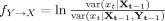 , which is the basis of the pGCM method.
The above time domain definition is not easily implemented in practice as it involves fitting separate autoregressive models to X t and Z t and to X t, Y t, and Z t. Estimation error and uncertainty in model parameters can arise in this process for finite data that may lead to uninterpretable results [Chen et al.,2006]. Here we consider a spectral domain procedure where a single autoregressive model is fit to X t, Y t, and Z t. [Chen et al.,2008] and the conditional causality spectrum is derived by combining Geweke's theory with spectral matrix factorization [Dhamala et al.,2008]. Time domain conditional Granger causality defined in Eq. (1) is obtained by integrating the spectrum over frequency.
The multivariate data W t = [w 1t, w 2t, …, w nt]T is modeled as a stationary VAR process:
 |
(2) |
where, A ijk is the AR coefficient between channels i and j at lag k and constitutes the ijth element of the AR coefficient matrix A k, where εt is a white noise residual with zero mean and covariance matrix Σ, and m is the order of the model, which can be determined by criteria, such as Akaike Information Criterion or Bayesian Information Criterion [Ding et al.,2006]. After Fourier transforming the above equations and suitable ensemble averaging, one gets the overall spectral matrix according to
| (3) |
where,  is the transfer function.
Geweke's spectral formulation of Granger causality (both pairwise and conditional) is based on the quantities in Eq. (3). Details are omitted but can be found in Geweke (1982, 1984), Chen et al. (2006, 2008), and Ding et al. (2006). For conditional causality estimation, the essence is the comparison between the model of two vector time series [numerator in Eq. (1)] and that of a three vector time series [denominator in Eq. (1)]. To avoid fitting AR models twice, thereby eliminating the problems associated with such repeated fitting, we choose suitable entries from the spectral matrix in Eq. (3) to form a new spectral matrix that corresponds to X t and Z t. Mathematically, it has been proven that this new spectral matrix can be factorized into a transfer function and the covariance matrix of the corresponding noise terms [Wilson,1972]. The two sets of spectral matrices and their associated H and Σ are then used to compute the spectral representation of Granger causality from Y t to X t conditioned on Z t. Integrating the spectrum over frequency yields the time domain counter, which is used throughout this work.
Significance Testing
A permutation procedure was used for the test of statistical significance of the computed cGCM [Brovelli et al.,2004; Nichols and Holmes,2001]. Specifically, 500 synthetic datasets were created by random rearrangement of the realization (subject/task) order independently for all vectors. Conditional Granger causality was computed for each permutation. A distribution of Granger causality values in time domain was obtained. For a given P‐value, a threshold was found from the distribution. The Granger causality values under the thresholds were considered not significant.
PCA‐cGCM Algorithm
For convenience, we summarize the general procedure for computing multivariate conditional Granger causality analysis as follows:
-
1
Obtain the statistical brain activation map from the fMRI data, using Brain Voyager QX (or other tools).
-
2
Select the reference ROI and perform PCA to yield a new vector time series of PCs, which account for most of the variance.
-
3
Select a target voxel in an activated brain region and treat the remaining voxels as a single block.
-
4
Extract a set of principle components from the block.
-
5
Calculate the conditional Granger causality from the reference ROI to the above selected voxel conditioned on the remainder block.
-
6
Repeat Steps (3)–(5) for all voxels in the activated brain regions.
SIMULATION
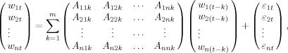
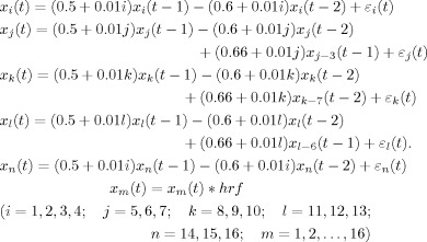
A 6 × 6 grid of voxels (Fig. 1a) was used to emulate a brain slice. Five different ROIs in the slice were denoted P, Q, S, R, and O. As shown in Figure 1b, region P was considered a primary area directly responding to the sequence of stimuli, which drove region Q after a 1 unit (3 s) of time delay and region S after 2 units of delay. Q, in turn, drove R after 1 unit of time delay. To simulate a likely functional situation, the 16 voxels/channels belonging to the activated regions were individually filtered by the convolution between the stimuli evolution and a linear model of the hemodynamic response function based on a gamma function. The tau parameter in the model was set to 0.5 corresponding to short stimulus durations. Then this simulation system contains two typical subsystems, which are a sequential driving model [P(t), Q(t), R(t)] and a distinct delayed driving model [P(t), Q(t), S(t)]. The voxel time series in each ROI come from one of the following coupled autoregressive processes:
 |
(4) |
where, εm(t), (m = 1, 2, …, 16), are independent Gaussian white noise processes with zero means and variances σ(t), and each time step is assumed to be 3 s. The specific region of interest assignment was: P(t) = [x 1(t); x 2(t); x 3(t); x 4(t)], Q(t) = [x 5(t); x 6(t); x 7(t)], S(t) = [x 8(t); x 9(t); x 10(t)], R(t) = [x 11(t); x 12(t); x 13(t)], and O(t) = [x 14(t); x 15(t); x 16(t)]. A data set of 12 realizations each with 120 time points was generated. To mimic the typical sampling rate of fMRI data, every point of each simulated time series was taken, corresponding to a repetition time of RT = 3 s. All methods were implemented in a Matlab environment on a PC (Intel R Core 2, 1.67 GHz CPU, and 2 Gb RAM).
Figure 1.
(a) Synthetic fMRI 6 × 6 voxels slice used for the validation of the PCA‐cGCM method. The slice simulates four functionally activated regions (P, Q, R, and S) and one deterministic region (O) not associated with the presumed task. Region P, which is composed of four voxels, is considered as the primary area directly activated by the stimuli; and the other three functional regions (Q, R, and S) are causally related with the region P. All the other voxels not included in the above five regions are the background regions. (b) Schematic illustration of a four‐node network, including a simple delay driving system (P, Q, and S) and a simple sequential driving system (P, Q, and R). (c) Granger causality network identified by pGCM analysis.
Region P was chosen as the reference region and its causal influence on each of the remaining voxels was calculated by pGCM and PCA‐cGCM. Figure 2a shows the pGCM result. As can be seen, the connections P → S and P → Q were correctly identified. However, the P → R influence is clearly spurious, indicating that pGCM could not resolve the indirect causality mediated by Q. For the application of PCA‐cGCM, the causality from P to each voxel conditioned on the remaining voxels was shown in Figure 2b. Again P → S and P → Q were correctly identified. More importantly, the P → R influence was removed, demonstrating the recovery of the true network connectivity underlying the simulation model (Fig. 1b).
Figure 2.

Granger causality analysis results from the synthetic fMRI data of the single 6 × 6 slice. Region P is the reference area, which includes four voxels with time courses defined by the stimuli sequence, regions Q, R, and S are three target areas, including three voxels each. The color bar indicates the value of Granger causality and each voxel's color stands for the causality value from region P to each voxel. (a) Granger causality mapping result of synthetic data by the pGCM method. (b) Granger causality mapping result of synthetic data by the PCA‐cGCM method. For both methods, Granger causalities in target regions were found related to the reference region, but different maps show the decrease in influence values with the PCA‐cGCM method (b) compared with the pGCM method (a). Obviously no causality was found from region P to region R based on the cGCM method.
Next we analyzed the interaction between each distinct pair of ROIs with pGCM and PCA‐cGCM. Fitting a second order VAR model [Ding et al.,2000] to the simulated data set, the results are shown in Figure 3. For pGCM, the identified connectivity pattern is shown in Figure 1c. Specifically, non‐zero Granger causality values were found for P(t) → R(t) and Q(t) → S(t), which is clearly spurious when compared with the model network in Figure 1b, again demonstrating the inability of the pGCM method in revealing true system relations. In contrast, the PCA‐cGCM approach was shown to identify the correct model network configuration. Here for each pair of ROIs the Granger causality values were computed with the remaining vectors in the network conditioned out. Indirect causal influences were eliminated with the cGCM (as shown in Fig. 3) and the sequential driving pattern as well as differential delays driving pattern were all clearly resolved. We believe that the benefits offered by the PCA‐cGCM method will be substantial when real fMRI data are analyzed to characterize functional networks in the human brain.
Figure 3.
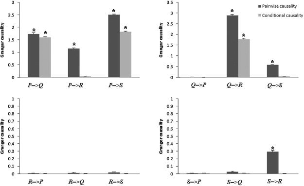
Time domain Granger causality results for four functional regions (P, Q, R, and S), using cGCM and pGCM methods. Charcoal grey bar is the pairwise causality results based on pGCM method and light grey bar is the conditional causality results based on cGCM method in each subgraph. *P < 0.05. Vertical bars indicate estimated standard errors.
Each ROI can be represented by its entire set of voxel time series, a single average time series or a set of PCs. The use of different representations can affect the quality of the result and the computation time. For a specific pair of ROIs P(t) and R(t), we compared pGCM and cGCM in the frequency domain, using each of the three aforementioned representations. In Figure 4a,b, a strong influence was found from P(t) to R(t) but little influence from R(t) to P(t) was detected, using the pGCM method based on original vector values, PC vector values and average values. As indicated earlier, this is a spurious result. The PCA gave a concise representation of each ROI. When combined with the cGCM method (PCA‐cGCM), correct network configuration was identified (Fig. 4c,d), namely, no direct causality was found between P(t) and R(t). Similar results were also found, by using the entire set of time series within each voxel (cGCM + Original). However, the use of average time series gave poor results (cGCM + AVG), indicating that average time series loses information and is not a good representation of ROI activity.
Figure 4.
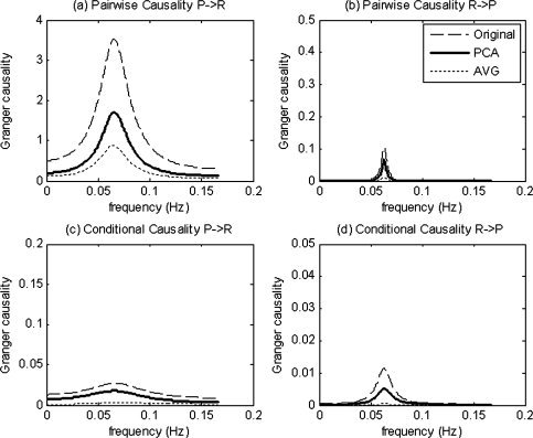
Frequency domain Granger causality results between region P and region R of the multivariate analysis; PCA‐cGCM and pGCM methods were applied to original vector values, principal components and average values. Dashed line indicates the result based on original vector values, bold solid line indicates the result based on principal components vectors, and the dotted line indicates the result based on average values.
The computation costs from the PCA‐cGCM and cGCM + AVG methods are much less than the computation costs, using the original voxel values (Table I). For real fMRI data, activated clusters always include a large number of voxels. It is thus difficult to apply the Granger causality method to the voxel time series directly. The proposed PCA‐cGCM method can solve this problem. Although the conditional method needs more time than the pairwise method, the benefit of distinguishing direct from outweighs this weakness. It is worth noting that these cost comparisons are only valid for the present example. More general claim can be made after a more thorough investigation.
Table I.
Causality recognition rate and time cost comparison using different strategies
| Methods | Recognition rate (%) | Computation time (s) |
|---|---|---|
| pGCM + AVG | 75% (9/12) | 2.130 |
| pGCM + Original | 75% (9/12) | 2.610 |
| pGCM + PCA | 75% (9/12) | 2.352 |
| cGCM + AVG | 83.3% (10/12) | 120.528 |
| cGCM + Original | 100% (12/12) | 715.386 |
| cGCM + PCA | 100% (12/12) | 287.052 |
ANALYSIS OF HUMAN fMRI DATA
Subjects
Twelve right‐handed volunteers with normal vision were recruited. The subjects did not report any neurological or psychiatric history and were not on psychoactive medications in the previous 6 months. The Granger analysis results from two subjects are reported here to illustrate our method. The analysis of data from all the subjects will be presented elsewhere. The research protocol for the human study was approved by the University of Florida's Institutional Review Board.
Task
The subjects performed a face matching task. Three conditions were used: (1) emotion condition, in which participants were asked to match faces by their expressed emotion (happiness, fear, or anger) from a target face to two probe faces positioned below the target face; (2) identity condition, in which participants were asked to match the identify of neutral faces; (3) control condition, in which the participant was asked to match pixilated patterns derived from neutral face pictures. The task was ordered in blocks of six 3‐s trials of the same condition, preceded by a 3‐s instruction screen. The block condition was presented in a fixed sequence that repeated four times. The entire run, lasting 369s, consisted of twelve 21‐s task blocks interspersed with thirteen 9‐s rest blocks [for detailed fMRI protocol see Wright and Liu,2006].
Imaging Protocol
The fMRI data was collected with a Siemens Allegra 3.0 Tesla MR scanner (Siemens, Munich, Germany) with a dome‐shaped standard head coil. Structure images were acquired using a T1 MPRAGE sequence in the sagittal plane at 1.0 mm3 resolution, TR = 1,780 ms, TE = 4.38 ms, flip angle = 8°. Functional images were acquired using a T2* weighted echo planar imaging BOLD sequence in the axial orientation (parallel to the AC‐PC line), covering the entire brain with 36 slices, 3.8 mm thick with no gap using TR = 3,000 ms, TE = 30 ms, flip angle = 90°, a 240 mm2 FOV and a 64 × 64 voxel matrix, resulting in a 3.75 mm in‐plane resolution. A total of 125 volumes were scanned during the matching task experiment and the first two volumes were discarded before analysis to allow for T1 equilibration.
Preprocessing and General Linear Model Analysis
Imaging data were analyzed using Brain Voyager QX (Brain Innovation, Maastricht, Netherlands). Anatomic and functional images were coregistered and normalized to Talairach space [Talairach and Tournoux,1988] for the subjects. Functional images underwent 3D motion correction, linear trend removal, and slice timing correction. Spatial smoothing was applied using a Gaussian filter of 6.00 mm full‐width half maximum and no temporal smoothing was applied to the functional data. Regional activations were estimated using a general linear model. Statistical maps based on group activation pattern with 12 subjects [Wright and Liu,2006] were created using random effects analysis. Individual voxel time series were regressed onto the model combined with these predictors, and clusters of voxels with significant differences between predictors had a statistical threshold of t(11) ≥ 4.0 (P < 0.002) and a minimum cluster size of 100 mm3. Two experimental conditions (Emotion and Identity) were contrasted with the control condition to identify activation within specific brain regions. The primary significant differences in modeled signal activations are summarized in Table II.
Table II.
Clusters of activation
| Region | Hemisphere | Brodmann area | Talairach coordinates | Size (mm3) | T score |
|---|---|---|---|---|---|
| Emotion > identity and control | |||||
| Inferior frontal sulcus | L | 9/44 | −44, 17, 30 | 208 | 5.1 |
| Precentral gyrus | R | 4 | 51, −3, 53 | 162 | 5.0 |
| Pregenual cingulated gyrus | L | 24/32 | −3, 38, 9 | 180 | −4.8 |
| Emotion and identity > control | |||||
| Amygdala | R | N/A | 23, −6, −9 | 510 | 6.2 |
| Subgenual cingulate gyrus | R | 32 | 4, 38, −7 | 120 | 5.3 |
| Fusiform gyrus | R | 37 | 40, −41, −18 | 248 | 5.1 |
| Inferior temporal sulcus | R | 37 | 49, −70, −3 | 293 | 6.2 |
| Middle temporal gyrus | R | 39 | 54, −58, 11 | 1,005 | 8.6 |
| Posterior cingulated gyrus | R | 23 | 2, −55, 25 | 1,770 | 6.0 |
Minimum cluster size: 100 mm3.
“Emotion > identity and control” was a conjunction of “Emotion > identity” and “Emotion > control.”
“Emotion and identity > control” was a conjunction of “Emotion > control” and “Identity > control.”
Granger Causality Analysis
To investigate the brain network underlying emotional processing, the BOLD signal from the region of the right amygdala activated during the emotion condition was used as a reference for calculating causality to all the other voxels in the brain imaging data. The PCA‐cGCM method treated all voxels except for those in the amygdala and the target voxel as a combined region to be conditioned out. PCA was used for dimensionality reduction for the reference region and the combined region. To assign significance levels to the computed measures a permutation procedure was applied [see Methods section]. The significance thresholds corresponded to P < 0.05.
The difference maps of conditional Granger causality were individually shown for the two subjects, respectively (Fig. 5 for Subject I and Fig. 6 for Subject II). The difference maps for each subject demonstrate two directions: (1) the amygdala → other activated voxels (Figs. 5a–c and 6a–c); and (2) other activated voxels → the amygdala (Figs. 5d–f and 6d–f). The difference maps from these two subjects are mostly consistent, which allows the determination of direct causal relations between the reference region, right amygdala, and other brain regions (or voxels) activated during the task. The pattern of such interactions shown in our results is in agreement with the findings in the previous studies using various approaches [Etkin et al.,2006; Johansen‐Berg et al.,2006; Mayberg,2003; Ochsner and Gross,2005; Vogt,2005]. It should be emphasized that the integrated PCA method is crucial in enabling a whole brain mapping at a reasonable computational cost.
Figure 5.
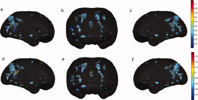
Mapping of the causal relationship during emotional processing for Subject I. The reference region is defined as the right amygdala. Causalities between the reference region and each voxel in activated regions, while conditioning out the remaining voxels in the brain were calculated. (a–c) Show the causalities from regions to the right amygdala. (d–f) Show the causalities from the right amygdale to other activated regions. The color bar indicates the value of causality.
Figure 6.

Mapping of the causal relationship during emotional processing for Subject II. The reference region is defined as the right amygdala. Causalities between the reference region and each voxel in activated regions, while conditioning out the remaining voxels in the brain were calculated. (a–c) Show the causalities from regions to the right amygdala. (d–f) Show the causalities from the right amygdale to other activated regions. The color bar indicates the value of causality.
DISCUSSION
Mapping functional neuroconnectivity is an essential step toward unraveling the brain mechanisms of cognition and emotion. Recently, effective connectivity with directional influences from on brain region to the other has been extracted from fMRI data based on the fMRI hemodynamic signals instead of neural activity signals [Goebel et al.,2003; Valdés‐Sosa et al.,2005]. However, the established pGCM method has two drawbacks: (1) it is not able to clearly distinguish direct from indirect causal relationships, and (2) it is computationally intensive. Efforts have been undertaken to address various aspects of this problem [Baccalá and Sameshima,2001; Eichler,2005; Valdés‐Sosa et al.,2005]. In this study, we have proposed a new approach combining PCA and cGCM. The method, referred to as PCA‐cGCM, was validated by using both simulation and in vivo fMRI data. Using simulated data, we showed that the PCA‐cGCM method can provide more detailed and accurate information than the traditional pGCM by distinguishing direct connectivity from indirect connectivity. Using fMRI data from human experiment, we were able to identify patterns of connectivity within a neural network implicated in emotional processing that were consistent with previous studies [Etkin et al.,2006; Johansen‐Berg et al.,2006].
Conditional Granger causality, by being able to differentiate direct from indirect causal influences, has been an essential method for linking network dynamics with network anatomy [Chen et al.,2006; Ding et al.,2006]. The incorporation of cGCM in functional connectivity imaging opens the possibility of better identifying the anatomical substrate that mediates cognitive and affective processing. A key issue in effective connectivity mapping is how to define ROIs and the assumable connections between them and how to represent the information in given ROIs in connectivity analysis. The classical pGCM method is often applied to single voxel time series or to ROI based average time series [Goebel et al.,2003; Roebroeck et al.,2005]. The former representation leads to high computational cost, while the latter representation is prone to information loss. The proposed approach performs a PCA analysis to extract components from a ROI based on the covariance structure of the data. These components account for most of the data variance but are much smaller in number when compared with that of the original voxel time series. Combining PCA with cGCM is shown to be effective in detecting network connectivity, while reducing the computational cost. Although these are preliminary observations, we are confident that the new method offers advantages over the classical methods.
In conclusion, our new analysis method based on PCA and conditional Granger causality has been shown to be useful in measuring complex effective connectivity with indirect influences from one brain region to the others. Most importantly, the use of PCA only leads to a minimum loss of information, which did not affect the connectivity analysis. The new method has a major strength in its ability to perform a direct connectivity mapping of the whole brain within a reasonable time frame. We thus suggest that the PCA‐cGCM technique is a potentially valuable tool to be used in the investigation of causality relations in brain connectivity studies.
REFERENCES
- Baccalá LA,Sameshima K( 2001): Partial directed coherence: A new concept in neural structure determination. Biol Cybern 84: 463–474. [DOI] [PubMed] [Google Scholar]
- Brovelli A,Ding M,Ledberg A,Chen Y,Nakamura R,Bressler SL ( 2004): Beta oscillations in a large‐scale sensorimotor cortical network: Directional influences revealed by Granger causality. Proc Natl Acad Sci USA 26: 9849–9854. [DOI] [PMC free article] [PubMed] [Google Scholar]
- Chen Y,Bressler SL,Ding M ( 2006): Frequency decomposition of conditional Granger causality and application to multivariate neural field potential data. J Neurosci Methods 150: 228–237. [DOI] [PubMed] [Google Scholar]
- Chen Y,Rangarajan G,Zhang Y,Ding M ( 2008): Assessing Neural Interactions with Granger Causality In: Tong S,Thakor N, editers. Quantitative EEG Analysis Methods and the Applications. Boston: Artech House. (in press) [Google Scholar]
- Dagher A,Owen AM,Boecker H,Brooks DJ ( 1999): Mapping the network for planning: A correlational PET activation study with the “Tower of London” task. Brain 122: 1973–1987. [DOI] [PubMed] [Google Scholar]
- Dhamala M,Rangarajan G,Ding M ( 2008): Analyzing information flow in brain networks with Nonparametric Granger Causality. NeuroImage 41: 354–362. [DOI] [PMC free article] [PubMed] [Google Scholar]
- Ding M,Bressler SL,Yang W,Liang H ( 2000): Short‐window spectral analysis of cortical event‐related potentials by adaptive multivariate autoregressive modeling: Data preprocessing, model validation, and variability assessment. Biol Cybern 83: 35–45. [DOI] [PubMed] [Google Scholar]
- Ding M,Chen Y,Bressler SL ( 2006): Granger Causality: Basic Theory and Applications to Neuroscience In: Schelter B,Winterhalder M, Timmer J, editors. Handbook of Time Series Analysis. Weinheim: Wiley‐VCH; pp. 437–460. [Google Scholar]
- Eichler M ( 2005): A graphical approach for evaluating effective connectivity in neural systems. Philos Trans R Soc Lond B Biol Sci 360: 953–967. [DOI] [PMC free article] [PubMed] [Google Scholar]
- Etkin A,Egner T,Peraza MD,Kandel RE,Hirsch J ( 2006): Resolving emotional conflict: A role for the rostral anterior cingulate cortex in modulating activity in the amygdala. Neuron 51: 871–882. [DOI] [PubMed] [Google Scholar]
- Friston K ( 2002): Beyond phrenology: What can neuroimaging tell us about distributed circuitry? Annu Rev Neurosci 25: 221–250. [DOI] [PubMed] [Google Scholar]
- Geweke J ( 1982): Measurement of linear dependence and feedback between multiple time series. J Am Stat Assoc 77: 304–313. [Google Scholar]
- Geweke J ( 1984): Measures of conditional linear dependence and feedback between time series. J Am Stat Assoc 79: 907–915. [Google Scholar]
- Goebel R,Roebroeck A,Kim D,Formisano E ( 2003): Investigating directed cortical interactions in time‐resolved fMRI data using vector autoregressive modeling and Granger causality mapping. Magn Reson Imag 21: 1251–1261. [DOI] [PubMed] [Google Scholar]
- Granger CWJ ( 1980): Testing for causality: A personal viewpoint. J Econ Dyn Control 2: 329–352. [Google Scholar]
- Johansen‐Berg H,Behrens TEJ,Matthews PM,Katz E,Metwalli N,Lozano A ( 2006): Connectivity of a subgenual cingulate target for treatment‐resistant depression In: 12th Annual Meeting of Human Brain Mapping, Florence, Italy. [Google Scholar]
- Jolliffe I ( 1986): Principal Component Analysis. New York: Springer Verlag. [Google Scholar]
- Lee L,Harrison LM,Mechelli A ( 2003): A report of the functional connectivity workshop, Dusseldorf 2002. NeuroImage 19: 457–465. [DOI] [PubMed] [Google Scholar]
- Liu Y,Gao J,Liotti M,Pu Y,Fox PT ( 1999): Temporal dissociation of parallel processing in the human subcortical outputs. Nature 400: 364–367. [DOI] [PubMed] [Google Scholar]
- Londei A,Ausilio AD,Basso D,Sestieri C,Gratta CD,Romani GL,Belardinelli MO ( 2007): Brain network for passive word listening as evaluated with ICA and Granger causality. Brain Res Bull 72: 284–292. [DOI] [PubMed] [Google Scholar]
- Mayberg HS ( 2003): Modulating dysfunctional limbic‐cortical circuits in depression: Towards development of brain‐based algorithms for diagnosis and optimized treatment. Br Med Bull 65: 193–207. [DOI] [PubMed] [Google Scholar]
- Nichols TE,Holmes AP ( 2001): Nonparametric permutation tests for functional neuroimaging: A primer with examples. Hum Brain Map 15: 1–25. [DOI] [PMC free article] [PubMed] [Google Scholar]
- Ochsner NK,Gross JJ ( 2005): The cognitive control of emotion. Trends Cogn Sci 5: 242–249. [DOI] [PubMed] [Google Scholar]
- Ogawa S,Lee TM ( 1990): Oxigenation‐sensitive contrast in magnetic resonance image of rodent brain at high magnetic fields. J Magn Reson Med 14: 68–78. [DOI] [PubMed] [Google Scholar]
- Owen AM,Doyon J,Petrides M,Evans AC ( 1996): Planning and spatial working memory: A positron emission tomography study in humans. Eur J Neurosci 8: 353–364. [DOI] [PubMed] [Google Scholar]
- Polat K,Günes S ( 2007): Automatic determination of diseases related to lymph system from lymphography data using principles component analysis (PCA), fuzzy weighting preprocessing and ANFIS. Expert Sys Appl 33: 636–641. [Google Scholar]
- Roebroeck A,Formisano E,Goebel R ( 2005): Mapping directed influence over the brain using Granger causality and fMRI. NeuroImage 25: 230–242. [DOI] [PubMed] [Google Scholar]
- Sato RJ,Junior AE,Takahashi YD,Felix MM,Brammer JM,Morettin AP ( 2006): A method to produce evolving functional connectivity maps during the course of an fMRI experiment using wavelet‐based time‐varying Granger causality. NeuroImage 31: 187–196. [DOI] [PubMed] [Google Scholar]
- Soares‐Filho W,Manoel de Seixas J,Pereira Caloba L ( 2001): Principal component analysis for classifying passive sonar signals. ISCAS 2001. IEEE Int Symp Circuits Sys 3: 592–595. [Google Scholar]
- Song W,Shao X ( 1997): Robust PCA based on neural networks. In: Proceedings of the 36th Conference on Decision and Control, San Diego, CA. pp. 503–508.
- Talairach J,Tournoux P ( 1988): Co‐planar Stereotaxic Atlas of the Human Brain: 3‐Dimensional Proportional System, an Approach to Cerebral Imaging. New York, NY: Thieme. [Google Scholar]
- Valdés‐Sosa PA,Snchez‐Bornot JM,Lage‐Castellanos A,Vega‐Hernndez M,Bosch‐Bayard J,Melie‐Garca L,Canales‐Rodrguez E ( 2005): Estimating brain functional connectivity with sparse multivariate autoregression. Philos Trans R Soc B 360: 969–981. [DOI] [PMC free article] [PubMed] [Google Scholar]
- Vogt BA ( 2005): Pain and emotion interactions in subregions of the cingulate gyrus. Neuroscience 6: 533–544. [DOI] [PMC free article] [PubMed] [Google Scholar]
- Wilson GT ( 1972): The factorization of matricial spectral densities. SIAM J Appl Math 23: 420–426. [Google Scholar]
- Wright P,Liu Y ( 2006): Neutral faces activate the amygdala during the identity matching. NeuroImage 29: 628–636. [DOI] [PubMed] [Google Scholar]