Analysis of functional image analysis contest (FIAC) data with brainvoyager QX: From single‐subject to cortically aligned group general linear model analysis and self‐organizing group independent component analysis

Abstract

The Functional Image Analysis Contest (FIAC) 2005 dataset was analyzed using BrainVoyager QX. First, we performed a standard analysis of the functional and anatomical data that includes preprocessing, spatial normalization into Talairach space, hypothesis‐driven statistics (one‐ and two‐factorial, single‐subject and group‐level random effects, General Linear Model [GLM]) of the block‐ and event‐related paradigms. Strong sentence and weak speaker group‐level effects were detected in temporal and frontal regions. Following this standard analysis, we performed single‐subject and group‐level (Talairach‐based) Independent Component Analysis (ICA) that highlights the presence of functionally connected clusters in temporal and frontal regions for sentence processing, besides revealing other networks related to auditory stimulation or to the default state of the brain. Finally, we applied a high‐resolution cortical alignment method to improve the spatial correspondence across brains and re‐run the random effects group GLM as well as the group‐level ICA in this space. Using spatially and temporally unsmoothed data, this cortex‐based analysis revealed comparable results but with a set of spatially more confined group clusters and more differential group region of interest time courses. Hum. Brain Mapp, 2006. © 2006 Wiley‐Liss, Inc.

INTRODUCTION

BrainVoyager QX (http://www.BrainVoyager.com) is a software package for the analysis and visualization of structural and functional MRI (fMRI) data. The program runs on all major computer platforms including Windows, Linux, and Mac OS X. BrainVoyager QX provides an easy‐to‐use, interactive graphical user interface (GUI) on all platforms and its functionality can be extended via C/C++ plugins and automated via scripts. In order to obtain maximum speed on each platform, BrainVoyager QX has been programmed in C++ with optimized and highly efficient statistical, numerical, and image‐processing routines. The software includes hypothesis‐driven (univariate) and data‐driven (multivariate) analyses of fMRI time series, several methods to correct for multiple comparisons, and tools to run multisubject volume and surface‐based region‐of‐interest (ROI) analyses. The software also contains tools and algorithms for the automatic segmentation of the brain and for the reconstruction, visualization, and morphing (inflation, flattening, sphering) of the cortical surface. An important feature of the software is that the analyses of functional and anatomical data are highly integrated. Not only can each type of statistical map be easily projected on the surface rendering of a cortical reconstruction, but also individual anatomical information (as provided, e.g., by labeled cortical voxels and individual cortical gyral and sulcal patterns) is actively used in the statistical analysis of single‐subject and group fMRI data, with the scope of enhancing sensitivity and improving the spatial correspondence across brains (see below). Other advanced analyses available in BrainVoyager QX were not performed due to space limitations, including BOLD latency mapping [Formisano et al., 2002b] and effective connectivity analysis (Granger causality mapping, Roebroeck et al. [ 2005]).

In the present article we describe some of the methods implemented in BrainVoyager QX (v. 1.6) in the context of analysis of the Functional Image Analysis Contest (FIAC) 2005 dataset. The details of the dataset and the experimental design are described in Dehaene‐Lambertz et al. [ 2006].

First, we illustrate a standard analysis of the functional and anatomical data, including preprocessing, spatial normalization into Talairach space, hypothesis‐driven statistics of the block‐ and event‐related paradigms for a single subject (Subject 3), and the group data. Following this standard hypothesis‐driven analysis, we apply single‐subject data‐driven cortex‐based Independent Component Analysis (ICA) [Formisano et al., 2004] and a recently developed group‐level ICA technique [Esposito et al., 2005]. We compare the results of this data‐driven analysis approach with the results obtained with univariate hypothesis‐driven methods. Finally, we apply a high‐resolution cortical alignment method [Goebel, 2004] to improve the spatial correspondence across brains and perform a random effects group General Linear Model (GLM) and group ICA analysis using the cortically aligned brains.

SUBJECTS AND METHODS

Subjects

The original FIAC 2005 dataset includes data from 16 subjects. In this article we report the results of analyses performed individually on Subject 3 (single‐subject analysis) and on a cohort of 12 subjects (group analysis). We excluded Subject 5 (no anatomical scan was available), Subject 7 (data from one functional run was missing), and Subjects 8 and 12 (excessive motion, as estimated during preprocessing).

Preprocessing of Functional Data

The functional data (ANALYZE format) was loaded and converted into BrainVoyager's internal “FMR” data format. The following standard sequence of preprocessing steps was performed for the data of each subject.

Slice scan time correction

Slice scan time correction was performed using sinc interpolation based on information about the TR (2500 msec) and the order of slice scanning (ascending, interleaved).

Head motion correction

3‐D motion correction was performed to detect and correct for small head movements by spatial alignment of all volumes of a subject to the first volume by rigid body transformations. Estimated translation and rotation parameters were inspected and never exceeded 3 mm or 2°, except in Subjects 8 and 12, who were excluded from the analysis.

Drift removal

Following a linear trend removal, low‐frequency nonlinear drifts of 3 or fewer cycles (0.0063 Hz) per time course for the block‐ and 7 cycles (0.015 Hz) for the event‐related design time series were removed by temporal highpass filtering. Since event‐related responses have more energy at higher frequencies, we could apply a higher cutoff, making the filtering of low‐frequency content (linear and nonlinear drifts) more effective. Conversely, the more sustained responses in the block design have more energy at lower frequency and this requires more attention in filtering the low‐frequency content since using a higher cutoff may, besides reducing drifts, also reduce the power of the functional responses. A lowpass Gaussian temporal filter with full‐width at half‐maximum (FWHM) of two data points was applied to the block‐design datasets as well to achieve modest temporal smoothing.

Spatial smoothing

Modest spatial smoothing using a Gaussian filter (FWHM = 5 mm) was applied for the volume‐based analysis. No spatial smoothing was used for the cortex‐based analysis.

Preprocessing of the Anatomical Data

Intensity inhomogeneity correction and spatial transformations

The anatomical data (ANALYZE format) of each subject was loaded and converted into BrainVoyager's internal “VMR” data format (Fig. 1A). Since the data exhibited spatial intensity inhomogeneities, a correction method [Vaughan et al., 2001] was applied, which estimates a bias field by analyzing the change of white matter intensities over space (Fig. 1B). The data were then resampled to 1‐mm resolution (Fig. 1C) and transformed into AC‐PC and Talairach standard space (Fig. 1D). The three spatial transformations were combined and applied backward in one step to avoid quality loss due to successive data sampling. The two affine transformations, iso‐voxel scaling and AC‐PC transformation, were concatenated to form a single 4 × 4 transformation matrix m. For each voxel coordinates in the target (Talairach) space a piecewise affine “Un‐Talairach” step was performed, followed by application of the inverted spatial transformation matrix, m ⁻¹. The computed coordinates were used to sample the data points in the original 3‐D space using sinc interpolation.

Figure 1.

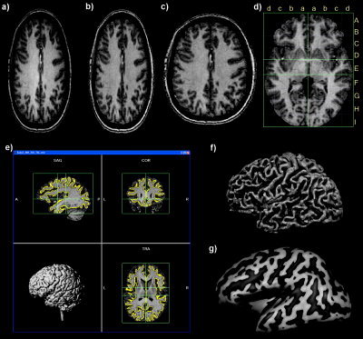
Anatomical preprocessing demonstrated with data from Subject 3. A: Selected slice of raw data as appearing in BrainVoyager QX after reading the raw anatomical 3‐D dataset. B: The same slice after inhomogeneity correction and removal of background noise. C: The same slice after application of a spatial transformation converting the voxels to isotropic 1‐mm voxels based on information in ANALYZE header. D: A slice through the AC‐PC plane after transformation of the dataset into Talairach space; the lines and letters represent the standard proportional grid system [Talairach and Tournoux, 1988]. For visualization purposes, head tissue has been automatically removed by running a brain segmentation tool (“brain peeling”). E: Result of cortex segmentation visualized in orthographic slices of the 3‐D data in Talairach space; the yellow lines indicate the segmented white/gray matter boundary of the two hemispheres. The lower left inset shows a volume rendering of the segmented brain. F: Visualization of the segmented cortex as a reconstructed mesh representation; convex curvature (reflecting mainly gyri) is colored in light gray, concave curvature (reflecting mainly sulci) is colored in darker gray. G: Visualization of an inflated representation of the cortex mesh.

Brain segmentation

For 3‐D visualization, the brain was segmented from surrounding head tissue using an automatic “brain peeling” tool. The tool analyzes the local intensity histogram in small volumes (20 × 20 × 20 voxels) to define thresholds for an adaptive region‐growing technique. This step results in the automatic labeling of voxels containing the white and gray matter of the brain, but also other high‐intensity head tissue. The next step consists of a sequence of morphological erosions to remove tissue at the border of the segmented data. By “shrinking” the segmented data, this step separates subparts, which are connected by relatively thin “bridges” with each other. By determining the largest connected component after the erosion step, the brain is finally separated from other head tissue since it constitutes the largest subpart. Finally, the sequence of erosions is reversed but restricted to voxels in the neighborhood of the largest connected component. This step re‐adds the tissue at the borders of the brain that was removed by the erosion step. Figure 1D shows a slice and Figure 1E a volume rendering of the brain after application of the brain segmentation tool.

Cortex segmentation

In order to perform a cortex‐based data analysis, the gray/white matter boundary was segmented using largely automatic segmentation routines [Kriegeskorte and Goebel, 2001]. Following the correction of inhomogeneities of signal intensity across space as described above, the white/gray matter border was segmented with a region‐growing method using an analysis of intensity histograms. Morphological operations were used to smooth the borders of the segmented data and to separate the left from the right hemisphere. If necessary, manual corrections were made to obtain correct segmentation results. This was necessary in the present data, especially in the upper part of the brains, due to a small white/gray matter contrast‐to‐noise ratio. More specifically, the segmented boundary in this region initially did not model the white/gray matter boundary but the outer (pial) boundary. Using optimized sequences [Howarth et al., 2006] and averaging two T1 scans of the same subject usually avoids this problem. Each segmented hemisphere was finally submitted to a “bridge removal” algorithm, which ensures the creation of topologically correct mesh representations [Kriegeskorte and Goebel, 2001]. The borders of the two resulting segmented subvolumes were tessellated to produce a surface reconstruction of the left and right hemisphere (Fig. 1F). With a fast, fully automatic 3D morphing algorithm [Goebel, 2000], the resulting meshes were transformed into inflated (Fig. 1G) and flattened (Fig. 2A) cortex representations. The original folded cortex meshes were used as the reference meshes for projecting functional data (maps and time courses) on inflated and flattened representations. A morphed surface always possesses a link to the folded reference mesh so that functional data can be shown at the correct location on folded, inflated, and flattened representations. This link was also used to keep geometric distortions to a minimum during inflation and flattening through inclusion of a morphing force that keeps the distances between vertices and the area of each triangle of the morphed surface as close as possible to the respective values of the folded reference mesh. For subsequent cortex‐based analysis, the folded cortex meshes were used to sample the functional data at each vertex (node), resulting in a mesh time course (“MTC”) dataset for each run of each subject.

Figure 2.

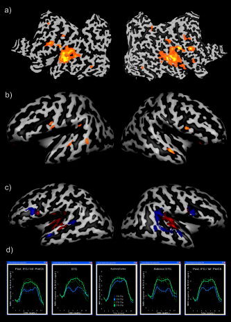
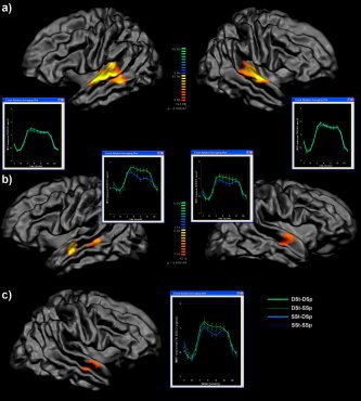
Hypothesis‐driven and data‐driven single‐subject analysis (Subject 3). A: Single‐subject, block design data, one‐factorial GLM analysis: main effects of auditory stimulation (F‐statistics, P = 0.05, Bonferroni corrected). B: Single‐subject, block design data, two‐factorial GLM analysis: t‐map (P = 0.01, α = 0.05) of sentence repetition effect. C: Single‐subject, block‐design data, cortex‐based ICA analysis: primary auditory component (red) and temporofrontal component (blue). D: Average time courses from selected ROIs of the block design data showing a strong stimulus‐related response in the auditory cortex (middle panel) and a strong speaker repetition effect in the superior temporal gyrus/sulcus and inferior frontal gyrus/sulcus (left and right panels). SSt = same sentence; DSt = different sentence; SSp = same speaker; DSp = different speaker.

Normalization of Functional Data

To transform the functional data into Talairach space, the functional time series data of each subject was first coregistered with the subject's 3‐D anatomical dataset, followed by the application of the same transformation steps as performed for the 3‐D anatomical dataset (see above). This step results in normalized 4‐D volume time course (“VTC”) data. In order to avoid quality loss due to successive data sampling, normalization was performed in a single step combining a functional‐anatomical affine transformation matrix, a rigid‐body AC‐PC transformation matrix, and a piecewise affine Talairach grid scaling step. As described for the anatomical normalization procedure, these steps were performed backward, starting with a voxel in Talairach space and sampling the corresponding data in the original functional space.

In the context of the functional‐anatomical alignment, some manual adjustment was necessary to reduce as much as possible the geometrical distortions of the echo‐planar images, which exhibited linear scaling in the phase‐encoding direction. The necessary scaling adjustment was done interactively using appropriate transformation and visualization tools of BrainVoyager QX.

Hypothesis‐Driven Analysis

Analysis steps

For each run of each subject's block and event‐related data, a BrainVoyager protocol file (PRT) was derived representing the onset and duration of the events for the different conditions. From the created protocols, one‐ and two‐factorial design matrices were defined automatically. In order to account for hemodynamic delay and dispersion, each of the predictors was derived by convolution of an appropriate box‐car waveform with a double‐gamma hemodynamic response function [Friston et al., 1998]. Using hypothesis‐driven, voxel‐wise standard analyses (GLM), we tested for overall task‐related effects to check general appropriateness of the analyses. This was followed by a GLM analysis of the 2 × 2 factorial design with three predictors testing for a sentence repetition main effect, a speaker repetition main effect, and a sentence × speaker interaction effect, respectively. One compact way to perform a 2‐factorial GLM analysis in BrainVoyager is to use the so‐called factorial design builder, which is based on the protocol definition and allows coding each single factor effect as well as each type of interaction effects as a separate predictor in the design matrix used in the GLM fit procedure.

We performed the GLM analysis in Subject 3 (Fig. 2A–B: block data) and in the group of 12 subjects after transformation in the conventional Talairach space (random effects results; Fig. 3A: block data; Fig. 3B–C: event‐related data). After fitting the GLM and accounting for the effects of temporal serial correlation (using AR(1) modeling; see Bullmore et al. [ 1996]), group or individual t‐maps of sentence repetition, speaker repetition, and sentence × speaker interaction were generated. For group‐level GLM analyses, we used a standard two‐level (hierarchical) ordinary least squares (OLS) fit procedure. Given the balanced design of the study and a sufficient number of trials, the OLS solution is expected to be very similar to a mixed‐effects solution. Thresholding of these maps with appropriate correction for multiple comparisons can be performed in various ways in BrainVoyager QX, including the false discovery rate (FDR) [Genovese et al., 2002] approach. Here we used a recently implemented approach based on a 3D extension of the randomization procedure described in Forman et al. [ 1995] for multiple comparison correction. First, a voxel‐level threshold was set at t = 3.1 (P = 0.01, uncorrected). Thresholded maps were then submitted to a whole‐brain correction criterion based on the estimate of the map's spatial smoothness and on an iterative procedure (Monte Carlo simulation) for estimating cluster‐level false‐positive rates. After 1,000 iterations, the minimum cluster size threshold that yielded a cluster‐level false‐positive rate (alpha) of 5% was applied to the statistical maps. The implemented method corrects for multiple cluster tests across space. For each simulated image, all “active” clusters in the imaged volume are considered and used to update a table reporting the counts of all the clusters above this threshold for each specific size. After a suitable number of iterations (e.g., 1,000), an alpha value is assigned to each cluster size based on its observed relative frequency. From this information the minimum cluster size threshold was specified in order to yield a cluster‐level false‐positive rate of α = 5%.

Figure 3.

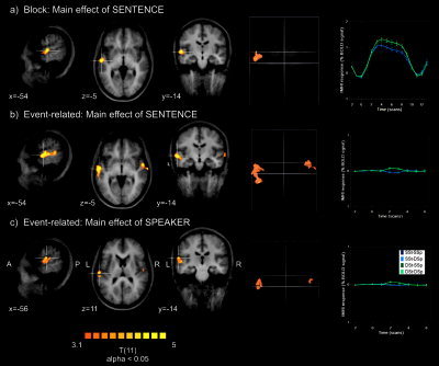
Two‐factorial GLM group‐level random effects analysis (12 subjects, Talairach space). A: Block design, sentence repetition effect. B: Event‐related design: sentence repetition effect. C: Event‐related design: speaker repetition effect. T‐maps (P = 0.01, α = 0.05, see text) are projected on the average of normalized individual brains (first three columns). Activated clusters are also shown in a glass‐brain view (fourth column). The fifth column shows the time course in active regions indicated by the white cross on the left.

RESULTS

Figures 2 and 3 and Table I summarize the main results of the hypothesis‐driven GLM analysis. Group analysis of “block” data showed a significant main effect of sentence repetition in the left anterior superior temporal sulcus and gyrus (STS/STG, Talairach coordinates of the peak: −56, −13, 1, Fig. 3A). A similar effect was also evident in the data of Subject 3, which was analyzed individually (Fig. 2B).

Table I.

Summary of GLM results in Talairach space

Area	Cluster size (mm3)	t(11) (peak)	Talairach coordinates x,y,z
Main effect of sentence repetition (block design)
Left anterior STS/STG	1701	7.11	−56, −13, 1
Speaker × sentence interaction effect (block design)
Left temporo–occipital cortex	904	4.64	−54, −46, −23
Right temporo–occipital cortex	603	4.87	39, −64, −27
Main effect of sentence repetition (event‐related design)
Left STS/STG	5119	7.31	54, −4, −5
Right STS/STG	2088	5.56	−58, −10, −2
Main effect of speaker repetition (event‐related design)
Left STS/STG	2006	6.82	49, −12, 11
Right STS/STG	239	4.12	−58, −19, 14

STG: superior temporal gyrus; STS: superior temporal sulcus.

In the group analysis of the block data, there was also a significant sentence‐by‐speaker interaction (map not shown) ventrally in the left and in the right temporal‐occipital cortex (−54, −46, −23, and 39, −64, −27). However, the amplitude of the average BOLD responses to each condition in these regions was much smaller than in STS/STG.

Group analysis of event‐related data showed a similar but more extended and bilateral main effect of sentence repetition in the left and right STS/STG (−58, −10, −2, and 54, −4, −5, Fig. 3B). In addition, there was also a main effect of speaker repetition located in the STG but more superiorly (−58, −19, 14, and 49, −12, 11, Fig. 3C).

Data‐Driven Analysis

Analysis steps

Single‐subject ICA [Formisano et al., 2002a, b, 2004] and Group ICA [Esposito et al., 2005] were applied to the first run of the block design experimental time‐series. The data of Subject 3 were used for the single‐subject cortex‐based ICA analysis and the whole sample of 12 subjects was used for the volume‐based and cortex‐based group‐level analysis in Talairach space and in the aligned cortical space (see below), respectively.

Individual and self‐organizing group‐level ICA were applied to the preprocessed functional time series using two C++ plugin extensions of BrainVoyager QX. The single‐subject ICA plugin implements methods described in Formisano et al. [ 2002a, b, 2004] and includes a C++ implementation of the fastICA algorithm [Hyvärinen and Oja, 2001; Esposito et al., 2002]. Prior to the ICA decomposition, the initial dimensions of the functional dataset were reduced from 191 (i.e., number of timepoints) to 40 using principal component analysis (PCA), which corresponded to more than 20% of the initial temporal dimensions and accounted in all subjects for more than 99.9% of the total variance‐covariance.

Individual ICA (Fig. 2C) detected two consistently task‐related components, one including bilaterally primary and secondary auditory cortex regions and one including a more distributed temporofrontal circuit, with clusters located along the superior temporal sulci and gyri (STS/STG) and in the inferior frontal gyri (IFG). The time courses of activity of both components were positively correlated with auditory stimulation in all four conditions, but only the temporofrontal component demonstrated a substantial adaptation effect during the sentence repetition and speaker repetition intervals. The amplitude of the component time course was higher during the blocks with different sentences and different speakers than during the blocks with the same sentences.

The ICA decompositions obtained from the datasets of each subject were submitted to the self‐organizing group ICA (sogICA) procedure, which has been implemented as a C++ plugin in BrainVoyager QX according to the methods and component clustering algorithm described in Esposito et al. [ 2005]. In this framework, the independent components from individual datasets are “clustered” at the group level. The clustering algorithm is based on components' mutual similarity measures implemented as linear spatial correlations in a common anatomical space. The common space may be either the voxels of a whole‐brain mask defined in the resampled Talairach volume or vertices from cortical surface meshes resampled on the standard sphere linked to each other by the cortex‐based alignment procedure (see below). In general, the sogICA framework allows the similarity matrix to be a combination of spatial and temporal measures. Using pure spatial similarity allows investigation of the consistency of independent components in a group of subjects despite the timing of experiments (e.g., differences in stimulus presentation across subjects). The similarity matrix is then transformed into a dissimilarity matrix, which is used as a “spatial distance” matrix within a hierarchical clustering algorithm [see also Himberg et al., 2004]. Cluster “group” components were calculated as random effects maps. The random effects statistic for each voxel was calculated as the mean ICA z‐value of that voxel across the individual maps divided by its standard error, resulting in a t‐statistic, which was converted to a z‐statistic. The resulting map of z‐values was visualized using a threshold of z = 2.2 (P = 0.0139, one‐sided). The cluster size in the subject component space was set to 12 components per subject. Thus, components with maximal spatial consistency across the whole sample of 12 analyzed subjects were extracted first and ranked high with respect to the mean intracluster similarity.

Results

Figure 4 shows the results of sogICA. Self‐organizing group‐level ICA identified a number of neurophysiologically meaningful group components, whose selection was facilitated by the ranking of the clusters given by the intracluster similarity measures. Among the first 10 clusters, we found the consistently task‐related component of early auditory processing, mainly focused in primary and secondary auditory regions (Fig. 4A, red component), and at least four other nontask‐related or negatively task‐related components, a parietofrontal component (Fig. 4A, cyan component), a parieto‐cingulate component (Fig. 4A, yellow component), an occipital component (Fig. 4A, green component), and a sensory‐motor component (Fig. 4A, purple component). These components reflect known circuits of functional connectivity and include the so‐called “default‐mode” network [Raichle et al., 2001; Grecious et al., 2004].

Figure 4.

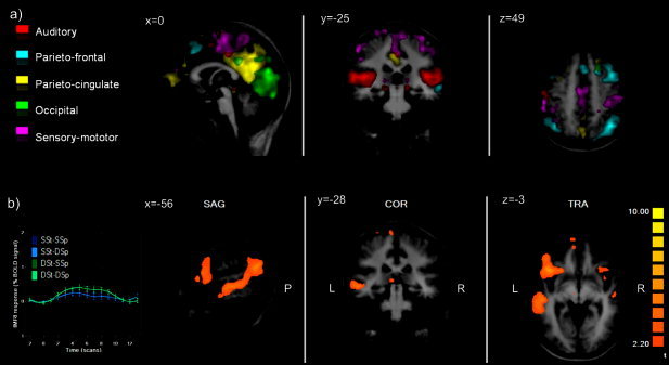
Self‐organizing group‐level ICA analysis (12 subjects, Talairach space). A: Auditory component (red), parietofrontal component (cyan), parieto‐cingulate component (yellow), occipital component (green), sensory‐motor component (purple) (t‐maps, P = 0.01). B: Temporofrontal component t‐map (P = 0.01) with group condition‐averaged time‐course showing a speaker repetition effect.

Most important for the repetition paradigm, we found a temporofrontal component (Fig. 4B) whose time course of activity was, again, positively and consistently correlated with auditory stimulation in all four conditions and exhibited the adaptation effect during the sentence repetition and speaker repetition intervals of stimulation. The spatial layout of this component was more lateralized in the left hemisphere and activated extended clusters along the STS/STG and the IFG.

Analysis in Aligned Cortical Space

A common cortical space potentially offers a more powerful group‐level functional data analysis due to a substantially improved anatomical alignment, which also improves the alignment of homologous functional regions (see below). Since gyri and sulci are not well aligned after standard Talairach or Montreal Neurological Institute (MNI) normalization procedures, suboptimal group results may be obtained since active voxels of some subjects will be averaged with nonactive voxels of other subjects due to pure alignment. In order to increase the overlap of activated brain areas across subjects, the functional data of each subject is extensively smoothed, typically with a Gaussian filter with an FWHM of 8–12 mm. While such an extensive spatial smoothing increases the overlap of active regions, it introduces other problems, including averaging of nonhomologous functional areas within and across subjects and the introduction of a bias for the statistical inference for clusters equal to or larger than the chosen Gaussian filter (matched filter theorem). The goal of cortex‐based alignment schemes is to explicitly align corresponding gyri and sulci across subjects in order to reduce these problems.

High‐resolution intersubject cortex alignment

While functional areas do not precisely follow cortical landmarks, it has been shown for areas V1 and motor cortex that a cortical alignment approach substantially improves statistical group results by reducing anatomical variability [Fischl et al., 1999]. In BrainVoyager QX, a high‐resolution, multiscale version of such a cortical mapping approach has been developed [Goebel et al., 2002, 2004], which automatically aligns brains using curvature information of the cortex. Since the curvature of the cortex reflects the gyral/sulcal folding pattern of the brain, this brain matching approach essentially aligns corresponding gyri and sulci across subject's brains. The implemented high‐resolution, multiscale cortex alignment procedure has been proven to substantially increase the statistical power and spatial specificity of group analyses [e.g., Van Atteveldt et al., 2004].

Cortex‐based alignment operates in several steps. The folded, topologically correct, cortex representation of each hemisphere (see Anatomical Preprocessing) constitute the input of the alignment procedure. In the first step, each folded cortex representation is morphed into a spherical representation (Fig. 5A), which provides a parameterizable surface well suited for across‐subject nonrigid alignment. Each vertex on the sphere (spherical coordinate system) corresponds to a vertex of the folded cortex (Cartesian coordinate system) and vice versa. The curvature information computed in the folded representation is preserved as a curvature map on the spherical representation. The curvature information (folding pattern) is smoothed along the surface to provide spatially extended gradient information driving intercortex alignment minimizing the mean squared differences between the curvature of a source and a target sphere. The essential step of the alignment is an iterative procedure following a coarse‐to‐fine matching strategy. Alignment starts with highly smoothed curvature maps and progresses to only slightly smoothed curvature representations. Starting with a coarse alignment as provided by AC‐PC or Talairach space, this method ensures that the smoothed curvature of the two cortices possess enough overlap for a locally operating gradient‐descent procedure to converge without user intervention [Goebel et al., 2002, 2004]. Visual inspection and a measure of the averaged mean squared curvature difference reveal that the alignment of major gyri and sulci can be achieved reliably by this method. Smaller structures, visible in the curvature maps with minimal smoothing, are aligned to a high degree but cannot be perfectly aligned due to anatomical differences between the subjects' brains.

Figure 5.

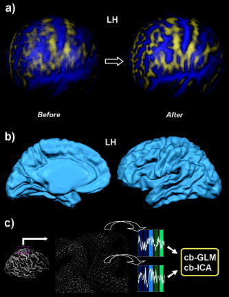
High‐resolution intersubject cortex alignment. A: Lateral view of left (LH) and right (RH) hemispheres before and after alignment of 12 subjects; for the cortical alignment, the 24 (2 × 12) cortices were morphed to a sphere. To visualize the correspondence between gyri and sulci, the curvature information of the cortices has been superimposed prior to and after alignment. B: Average cortex of left and right hemisphere of 12 subjects after cortex alignment; this representation is obtained by averaging 3‐D coordinates of vertices on the basis of the established correspondence mapping. C: Visualization of the creation of “mesh time courses,” which are used to run hypothesis‐driven (cg‐GLM) and data‐driven single and group analyses (cg‐ICA) directly in aligned cortex space.

The program offers two approaches to define a target brain for alignment. In the explicit target approach, one sphere is selected as a target to which all other spheres are subsequently aligned. The target sphere can be derived from one of the brains of the investigated group or from a special reference brain, such as the MNI template brain. Although tests have shown that achieved alignment results are very similar when using different target spheres, the selection of a specific target brain might lead to suboptimal results if the selected brain contains many regions with a nontypical folding pattern. In the moving target group averaging approach, the selection of a target sphere is not required. In this approach the goal function is specified as a “moving target” computed repeatedly during the alignment process as the average curvature across all hemispheres at a given alignment stage. The procedure starts with the coarsest curvature maps. Then the next finer curvature maps are used and averaged with the obtained alignment result of the previous level. Figure 5A shows the obtained result from the moving target alignment approach. The four spheres show the averaged curvature maps of the 12 cortices before and after alignment for the left and right hemispheres. Figure 5B shows a folded averaged cortex representation of the left and right hemisphere of 12 subjects after cortex alignment. This representation is obtained by averaging 3‐D coordinates of vertices of the folded meshes on the basis of the established correspondence mapping. This representation demonstrates the successful operation of the cortex‐based alignment approach, revealing an averaged cortex representation containing almost the same level of detail as each of the 12 individual brains.

The established correspondence mapping between vertices of the cortices is used to align the subjects' functional data. As described above, the functional time course data is attached to the vertices (nodes) of the cortex meshes by sampling the volume time courses (“VTCs”) at the vertex positions of the folded cortex meshes of each subject, resulting in a mesh time course (“MTC”) for each run of each subject's data (Fig. 5C). The fixed and random‐effects GLM and the group‐level ICA procedures work in the same way as in standard volumetric space but are modified to take as input the cortically aligned mesh time course data.

Hypothesis‐driven cortex‐based group analysis

The results of the cortex‐based random‐effects (RFX) group GLM analysis confirmed the volume‐based analyses in Talairach space. The results from the spatially unsmoothed block data is shown in Figure 6 superimposed on the average group cortex. The overall activation map (Fig. 6A) demonstrates the good alignment of the cortices of the 12 subjects by revealing activity confined within and around Heschl's gyrus (P < 0.01, corrected). A sentence repetition RFX effect (t(11) > 3.1, P < 0.01, uncorrected for multiple comparisons) was found bilaterally, with a more extensive region in the left STS than in the right STS. It can be seen from the averaged time course that the adaptation effect evolves over time, since the difference between the two different sentence (DSt) vs. the two same sentence (SSt) conditions is almost absent at the beginning but clearly visible towards the end of the block. This difference was also more pronounced in the clusters of the left STS than in the cluster of the right STS. While not significant, the largest trend for a speaker repetition effect was found in the right anterior STS (Fig. 6C).

Figure 6.

Hypothesis‐driven cortex‐based group‐level random effects analysis on spatially nonsmoothed mesh time courses (12 subjects, block data). A: Group map of overall stimulation vs. baseline superimposed on average group cortex mesh obtained from cortex‐based alignment procedure; time courses are drawn from regions around left and right Heschl's gyrus. B: Group map showing a strong sentence repetition effect in two clearly identifiable clusters in the superior temporal sulcus in the left hemisphere and a weaker sentence repetition effect in the anterior superior temporal sulcus and gyrus in the right hemisphere. C: Group map showing a weak speaker repetition effect (nonsignificant, see text) in the right anterior superior temporal sulcus and gyrus. The time course reveal that the small trend is more pronounced within the DSt (different sentence) conditions than the SSt (same sentence) conditions.

Data‐driven cortex‐based group analysis

Although unsmoothed functional data was used, the self‐organizing group‐level ICA in the spherically aligned cortex space produced highly consistent results with the volume‐based group ICA. Limiting our description to the two task‐related components, cortex‐based ICA provided a much more anatomically detailed picture of the same two‐component model at the group level than the Talairach space ICA. Figure 7 shows these components superimposed on the average cortex brain. The first task‐related component exhibited a consistently task‐related pattern of activation without a sentence or speaker repetition effect and encompassed the primary and secondary auditory regions (red overlay in Fig. 7); the second, frontotemporal, component (blue overlay in Fig. 7) exhibited again a substantial adaptation effect, but encompassed more precisely and more bilaterally the STS and the IFG than the volume‐based result.

Figure 7.

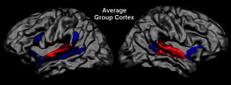
Data‐driven cortex‐based group‐level analysis. Results of the self‐organizing group‐level ICA. Auditory (red) and temporofrontal (blue) group components projected on the average group cortex mesh (t‐maps, P = 0.01).

CONCLUSIONS

The present study illustrates a range of processing methods and algorithms that are included in BrainVoyager QX and that can be used to analyze functional and anatomical MRI data. Our hypothesis‐driven analysis of the FIAC 2005 data in Talairach space revealed regions exhibiting a significant sentence repetition effect in the block data and significant sentence and speaker repetition effects in the event‐related data. The event‐related paradigm thus seems better suited to reveal a speaker effect than the blocked paradigm. It should be noted, however, that the strength of the sentence effect is substantially stronger than the speaker effect in both paradigms. We observed a trend toward a speaker effect. Without spatial smoothing of the functional data, the cortex‐based analysis confirmed the volume‐based analysis, providing, however, more focal clusters and more differential group ROI time courses, indicating an improved functional alignment. Group averaged time courses for the sentence repetition effect in the STS showed that this effect is almost absent at the beginning of a block and increases to reach its maximum roughly in the middle of the block.

The data‐driven ICA analysis complements the voxel‐wise statistical analysis by focusing on network‐related activity. The results of this analysis were surprisingly similar to the GLM results separating a main component in and around Heschl's gyri and a more widespread component in higher auditory cortices, insular, and frontal cortex. We think that the two‐component representation provided by the group ICA results reflects the functional role of each pattern in relation to early primary auditory processing of the sentences and higher‐level integration of sentence and voice‐related information processing. While consistent with the current models of language and voice processing [see, for instance, Belin et al., 2003, 2004], this representation provides a different and more distributed view of the neural processes elicited by the prolonged auditory stimulation. This functional connectivity model nicely complements the more localized and effect‐specific view of the studied effects provided by the conventional hypothesis‐driven statistical analysis of the same data.

REFERENCES

- Belin P, Zatorre RJ (2003): Adaptation to speaker's voice in right anterior temporal lobe. Neuroreport 14: 2105–2109. [DOI] [PubMed] [Google Scholar]
- Belin P, Fecteau S, Bedard C (2004): Thinking the voice: neural correlates of voice perception. Trends Cogn Sci 8: 129–135. [DOI] [PubMed] [Google Scholar]
- Bullmore E, Brammer M, Williams S, Rabe‐Hesketh S, Janot N, David A, Mellers J, Howard R, Sham P (1996): Statisticalmethods of estimation and inference for functional MR image analysis. Magn Reson Med 35: 261–277. [DOI] [PubMed] [Google Scholar]
- Dehaene‐Lambertz G, Dehaene S, Anton JL, Campagne A, Ciuciu P, Dehaene GP, Denghien I, Jobert A, LeBihan D, Sigman M, Pallier C, Poline JB (2006): Functional segregation of cortical language areas by sentence repetition. Hum Brain Mapp 27: 360–371. [DOI] [PMC free article] [PubMed] [Google Scholar]
- Esposito F, Formisano E, Seifritz E, Goebel R, Morrone R, Tedeschi G, Di Salle F (2002): Spatial independent component analysis of functional MRI time‐series: to what extent do results depend on the algorithm used? Hum Brain Mapp 16: 146–157. [DOI] [PMC free article] [PubMed] [Google Scholar]
- Esposito F, Scarabino T, Hyvarinen A, Himberg J, Formisano E, Comani S, Tedeschi G, Goebel R, Seifritz E, Di Salle F (2005): Independent component analysis of fMRI group studies by self‐organizing clustering. Neuroimage 25: 193–205. [DOI] [PubMed] [Google Scholar]
- Fischl B, Sereno MI, Tootell RBH, Dale AM (1999): High‐resolution inter‐subject averaging and a coordinate system for the cortical surface. Hum Brain Mapp 8: 272–284. [DOI] [PMC free article] [PubMed] [Google Scholar]
- Forman SD, Cohen JD, Fitzgerald M, Eddy WF, Mintun MA, Noll DC (1995): Improved assessment of significant activation in functional magnetic resonance imaging (fMRI): use of a cluster‐size threshold. Magn Reson Med 33: 636–647. [DOI] [PubMed] [Google Scholar]
- Formisano E, Esposito F, Kriegeskorte N, Tedeschi G, Di Salle F, Goebel R (2002a): Spatial independent component analysis of functional magnetic resonance imaging time‐series: characterization of the cortical components. Neurocomputing 49: 241–254. [Google Scholar]
- Formisano E, Linden DEJ, Di Salle F, Trojano L, Esposito F, Sack AT, Grossi D, Zanella FE, Goebel R (2002b): Tracking the mind's image in the brain. I. Time‐resolved fMRI during visuospatial mental imagery. Neuron 35: 185–194. [DOI] [PubMed] [Google Scholar]
- Formisano E, Esposito F, Di Salle F, Goebel R (2004): Cortex‐based independent component analysis of fMRI time‐series. Magn Reson Imaging 22: 1493–1504. [DOI] [PubMed] [Google Scholar]
- Friston KJ, Fletcher P, Josephs O, Holmes A, Rugg MD, Turner R (1998): Event‐related fMRI: characterizing differential responses. Neuroimage 7: 30–40. [DOI] [PubMed] [Google Scholar]
- Genovese CR, Lazar NA, Nichols T (2002): Thresholding of statistical maps in functional neuroimaging using the false discovery rate. Neuroimage 15: 870–878. [DOI] [PubMed] [Google Scholar]
- Goebel R (2000): A fast automated method for flattening cortical surfaces. Neuroimage 11: S680. [Google Scholar]
- Goebel R (2001): Cortex‐based alignment. Soc Neurosci Abstr.
- Goebel, R. , Singer, W (1999): Cortical surface‐based statistical analysis of functional magnetic resonance imaging data. Neuroimage Suppl [Google Scholar]
- Goebel R, Hasson U, Lefi I, Malach R (2004): Statistical analyses across aligned cortical hemispheres reveal high‐resolution population maps of human visual cortex. Neuroimage 22(Suppl 2) [Google Scholar]
- Himberg J, Hyvarinen A, Esposito F (2004): Validating the independent components of neuroimaging time series via clustering and visualization. Neuroimage 22: 1214–1222. [DOI] [PubMed] [Google Scholar]
- Howarth C, Hutton C, Deichmann R (2006): Improvement of the image quality of T1‐weighted anatomical brain scans. Neuroimage 29: 930–937. [DOI] [PubMed] [Google Scholar]
- Hyvärinen A, Oja E (2001): Independent component analysis. New York: John Wiley & Sons. [Google Scholar]
- Kriegeskorte N, Goebel R (eds.) (2001): An efficient algorithm for topologically correct segmentation of the cortical sheet in anatomical MR volumes. Neuroimage 14: 329–346. [DOI] [PubMed] [Google Scholar]
- Roebroeck A, Formisano E, Goebel R (2005): Mapping directed influence over the brain using Granger causality and fMRI. Neuroimage 25: 230–242. [DOI] [PubMed] [Google Scholar]
- Talairach J, Tournoux P (1988) Co‐planar stereotaxic atlas of the human brain. Stuttgart: G. Thieme. [Google Scholar]
- Van Atteveldt N, Formisano E, Goebel R, Blomert L (2004): Integration of letters and speech sounds in the human brain. Neuron 43: 271–282. [DOI] [PubMed] [Google Scholar]
- Vaughan JT, Garwood M, Collins CM, Liu W, DelaBarre L, Adrainy G, Andersen P, Merkle H, Goebel R, Smith MB, Ugurbil K (2001): 7T vs. 4T: RF power, homogeneity, and signal‐to‐noise comparison in head images. Magn Reson Med 46: 24–30. [DOI] [PubMed] [Google Scholar]