

Abstract
Memory encoding is a critical brain function subserved by the hippocampus (HP) and mesial temporal lobe (mTL) structures. Visualization of mTL memory activation with BOLD fMRI is complicated by the presence of static susceptibility gradients in this region. Arterial spin labeled (ASL) perfusion fMRI offers an alternative approach not dependent on susceptibility contrast that instead suffers from lower intrinsic signal‐to‐noise ratio. An improved ASL perfusion fMRI approach combining pseudo‐continuous ASL and a T2*‐insensitive sequence (GRASE) with background suppression was compared to BOLD fMRI at 3 T during a scene encoding task known to activate the HP. Overall, an approximate sixfold sensitivity increase of ASL fMRI was achieved, with improved coverage in the anterior mTL, while suppression of the static tissue enhanced the stability of the ASL series by a factor of 2.4. Perfusion fMRI using this approach with 4 mm isotropic resolution yielded better localized and stronger group activation maps than BOLD fMRI at a standard resolution of 3 mm isotropic voxels. Increasing the resolution for BOLD to 2.5 mm isotropic produced stronger mTL and hippocampal activation in the group and individual subjects than the ASL technique, due to superior temporal resolution and reduced partial volume effects. Future improvements in ASL spatial and temporal resolution would allow the benefits of both approaches to be combined to further enhance the sensitivity for detecting mTL activation during memory encoding. Hum Brain Mapp, 2007. © 2007 Wiley‐Liss, Inc.
Keywords: perfusion fMRI, arterial spin labeling, 3D GRASE, memory encoding, hippocampus
INTRODUCTION
Memory encoding is a critical brain function that is primarily subserved by the hippocampus (HP) and adjacent mesial temporal lobe (mTL) structures [Squire, 1992] and may be affected by a variety of brain disorders. The ability to localize and quantify memory encoding has several potential clinical applications, including presurgical assessment for temporal lobectomy performed for medically refractory temporal lobe epilepsy [Rabin et al., 2004] and for preclinical diagnosis of Alzheimer's disease [Bookheimer et al., 2000]. The most common approach for preclinical memory localization is the intracarotid amobarbital (Wada) test [Milner et al., 1962; Wada and Rasmussen, 1960], but this test has numerous shortcomings, most notably its invasiveness. Accordingly, the development of a noninvasive approach for assessment of memory encoding has been one of the major potential clinical applications of functional MRI (fMRI). However, although encoding tasks have successfully demonstrated functionally relevant activation of the mTL region [Brewer et al., 1998; Stern et al., 1996; Wagner et al., 1998], it has been much more difficult to reliably obtain activation in the HP proper. While some of this difficulty may be attributed to challenges in effectively modulating memory activity [Stark and Squire, 2001], much of the difficulty is thought to relate to challenges in obtaining good fMRI signal from this relatively small region in the presence of high static susceptibility gradients.
Several methods have been proposed to reduce signal loss due to susceptibility induced field gradients in gradient‐echo imaging sequences such as EPI, the most common sequence of choice for BOLD experiments. The simplest approach to implement is increasing voxel resolution, thereby reducing intravoxel dephasing [Young et al., 1988]. This approach has been shown to improve hippocampal activation at 1.5 T Fransson et al., 2001 and 3 T [Szaflarski et al., 2004]. Another method uses multiple refocusing gradients (z‐shim) to compensate for field inhomogeneities [Constable, 1995; Frahm et al., 1988; Ordidge et al., 1994]. High‐order field compensations can be achieved through specially tailored RF pulses [Cho and Ro, 1992]. Most of these approaches require pulse sequence modifications, which eliminate one advantage of BOLD, the easiness of implementation. In addition, some of these approaches reduce signal drop off in areas of high susceptibility contrast but decrease signal‐to‐noise ratio (SNR) in the regions of homogeneous field. Finally, some of these methods require multiple repetitions to obtain a uniform image, thus significantly increasing the acquisition time.
An alternative approach for fMRI in regions of high static susceptibility contrast is the use of arterial spin labeling (ASL) to directly measure changes in cerebral blood flow (CBF) during task activation. ASL does not depend on susceptibility contrast and offers several theoretical benefits for fMRI [Detre and Wang, 2002]. Although most ASL applications have still relied on echoplanar imaging, alternative approaches with reduced T2* sensitivity now also exist [Fernandez‐Seara et al., 2005]. While changes in CBF with task activation can be large, ASL techniques generally suffer from intrinsically low SNR when compared to the widely adopted BOLD contrast due to the small fraction of arterial blood to tissue in the human brain (1–2%) [Blinkov and Glezer, 1968]. Further, since the ASL signal change is typically less than 1% of the background signal intensity, physiological noise introduced by motion or other instabilities can have detrimental effects on the accuracy and precision of ASL measurements. High field strength has improved the SNR of ASL methods [Wang et al., 2002], but there is evidence suggesting that the physiological noise also increases, leading to no net gain in functional activation studies when compared to 1.5 T.
Suppression of the background (i.e. static tissue) signal can improve the sensitivity and reproducibility of the ASL signal, by reducing physiological noise at high field strengths [Duyn et al., 2001; Garcia et al., 2005b; Ye et al., 2000]. Background suppression (BS) is achieved by implementation of additional inversion pulses after the labeling of the arterial spins, during the postlabeling delay. The number of inversion pulses and their timing need to be optimized in order to achieve maximum suppression of the static signal with a minimal attenuation of the ASL signal. It has been recently shown that careful selection of the type of inversion pulses, their number, and their timing is crucial for efficient inversion in background suppressed ASL sequences [Garcia et al., 2005b]. After optimization, the efficiency of the inversion appears to be limited by a magnetization transfer process in blood, which causes the attenuation of the ASL signal. Although a slight decrease of the signal is expected, there is a net gain of stability and sensitivity in background suppressed ASL sequences.
Implementation of BS in 2D multi‐slice acquisitions is hampered by the different acquisition time of each slice. The use of a 3D single shot sequence for read‐out eliminates this problem, since the k‐space center is sampled simultaneously for the whole imaging volume. In addition, 3D sequences have intrinsically higher sensitivity than 2D multi‐slice sequences, since the signal from the whole volume is sampled for every excitation. We have previously shown [Gunther et al., 2005] that single shot 3D GRASE ASL images have higher spatial SNR than 2D EPI ASL. The multiple 180° RF refocusing pulses in GRASE maintain signal coherence for less signal decay and allow for a longer duration of signal readout, which gives several times as many signals in a longer echo train. Image reconstruction with this larger number of signals using 3D FT produces higher SNR than 2D FT EPI images. We have also demonstrated [Fernandez‐Seara et al., 2005] that a continuous ASL (CASL) sequence with a single shot 3D GRASE readout generates perfusion images that have less susceptibility artifact and signal drop out than those obtained with the 2D EPI readout, with better coverage in the orbito‐frontal cortex.
Continuous flow driven adiabatic inversion produces the largest ASL signal change [Wong et al., 1998], but the multi‐slice implementation of CASL with amplitude modulated control [Alsop and Detre, 1998] has an efficiency of approximately 70% due to imperfections of the control pulse. A more efficient pseudo‐continuous ASL (pCASL) approach for flow driven adiabatic inversion was recently described [Garcia et al., 2005a]. The pseudo‐continuous approach for flow driven adiabatic inversion has several advantages with respect to the amplitude modulated control technique. Since it is a pulsed approximation to CASL (i.e. it employs repeated RF pulses instead of continuous RF), it does not require continuous wave RF transmit capabilities. Thus, it permits the use of the body coil as transmitter and a phased‐array head coil as receiver, which increases the SNR of the raw images. Moreover, the pCASL approach increases the efficiency of the inversion for multi‐slice acquisitions, while controlling for magnetization transfer effects.
The goal of this study was to assess the performance of an optimized ASL perfusion fMRI sequence incorporating pCASL, BS, and single shot 3D GRASE and its utility for visualizing activation in the mTL and HP. The performance of the pCASL BS 3D GRASE sequence for detecting mTL activation was evaluated by comparison with BOLD fMRI during a well‐established memory encoding task, which we have previously used to activate mesial temporal structures [Detre et al., 1998] including the HP [Narayan et al., 2005]. For this comparison, BOLD fMRI was carried out at a “standard” resolution of 3 × 3 × 3 mm3 (3 mm isotropic) and at a “high” resolution of 2.5 × 2.5 × 2.5 mm3 (2.5 mm isotropic). The single shot 3D GRASE sequence used for imaging the effects of ASL provided a resolution of 4 × 4 × 4 mm3 (4 mm isotropic).
MATERIALS AND METHODS
All imaging studies were performed on a 3 T Trio whole‐body scanner (Siemens Medical Systems, Erlangen, Germany), with a maximum gradient strength of 40 mT/m and slew rate of 200 mT/(m msec), using the product 8‐channel head receiver array. Written informed consent was obtained prior to the human studies following an Institutional Review Board approved protocol. Thirteen healthy volunteers (mean age = 28 ± 10 [standard deviation], 7 females, 6 males) were scanned using both ASL and BOLD fMRI during the same session. An explicit memory encoding paradigm was administered as a blocked design consisting of task/control cycles of complex visual scenes or a scrambled scene control stimulus [Detre et al., 1998], presented on a back‐lit projection screen viewed through a mirror mounted on the head coil. Subjects were instructed to remember the task scenes but only attend to the control scrambled scene. Because the temporal resolution of our ASL sequence was approximately 7.5 s when compared to 3 s for BOLD, the experimental design was slightly different for the BOLD and ASL techniques in that a different block length was used. It has been previously shown that the noise characteristics of BOLD and perfusion data are different [Aguirre et al., 2002], and that ASL perfusion fMRI does not suffer from longer block durations [Kim et al., 2006; Wang et al., 2003]. Control and task blocks were interleaved starting with a control block, with each block lasting 135 s for ASL and 36 s for BOLD. The total duration was 9.25 min for both scans. The ASL scan was performed first, followed by the BOLD scan.
ASL was performed using a pCASL background‐suppressed single shot 3D GRASE sequence, shown in Figure 1. The imaging slab covered the temporal lobes. Imaging parameters were as follows: resolution = 4 mm isotropic, FOV = 250 × 204 × 48 mm3, 12 nominal partitions with 33% oversampling, 5/8 partial Fourier, measured partitions = 10, matrix size = 64 × 52, BW = 3,004 Hz/pixel, gradient‐echo spacing = 0.4 ms (with ramp sampling), spin‐echo spacing = 26 ms, total read‐out time = 270 m, effective TE = 52 ms, refocusing flip angle = 162°. A delay was introduced at the end of the GRASE readout so that TR was 3.75 s. The pCASL pulse [Garcia et al., 2005a] consisted of 1,280 selective RF pulses, played sequentially, at equal spacing, for a 1.2 s labeling duration. Each RF pulse was shaped as a modified Hanning window (peak/average B 1 = 53/18 mG, duration = 500 μs, and peak/average G = 0.6/0.23 G/cm). For the control pulse, the RF phase alternated from 0° to 180°. The inversion plane was offset 6 cm from the center of the FOV in the HF direction, so that it was located at the base of the cerebellum to achieve good labeling efficiency. The postlabeling delay was 400 ms. Two hyperbolic secant inversion pulses (15.35 ms duration and 220 mG RF amplitude) were added with inversion times of 1,590 and 380 ms, respectively, for BS (see the Appendix). The first pulse was applied selectively to the imaging slab while the second pulse was nonselective. The use of BS allowed an increase in receiver gain by a factor of 15, thus fully utilizing the dynamic range of the receiver. The pCASL pulse was placed in between the two BS pulses. Bipolar gradients (b = 5 sec/mm2) were added between the excitation and the first refocusing pulse of the GRASE readout to suppress intravascular signal. Seventy‐two perfusion images were obtained by pair‐wise subtraction of tag and control (after discarding four dummy scans).
Figure 1.

ASL pulse sequence diagram, showing the BS pulses (θ) with inversion times of 1,590 and 380 ms, respectively, and pCASL pulse of 1,200 ms duration, added to the single shot 3D GRASE readout. [Color figure can be viewed in the online issue, which is available at www.interscience.wiley.com.]
Prior to the perfusion fMRI scan, a short resting scan (five tag/control pairs) was performed with the same sequence parameters without BS. The acquired pairs were used to evaluate the performance of the BS pulses. This was done by comparing the spatial SNR of the control images and the temporal SNR (tSNR) of the perfusion images, with the spatial and tSNR of the first five pairs in the background suppressed series. The spatial SNR of the control images was computed as the signal mean measured in a region of interest (ROI) covering the whole imaging volume over the standard deviation of the signal in a ROI placed in the background. The degree of BS was calculated for every subject as the ratio of the spatial SNR of the suppressed to the unsuppressed mean control image. The tSNR of the perfusion images was calculated as the mean of the global perfusion signal (tag‐control) over the standard deviation of the time course.
The tSNR of the raw control GRASE image and the perfusion image time series was computed for the full series of 72 images, in a region covering the whole HP based on the Wake Forest Pickatlas utility [Maldjian et al., 2003], as well as in two hippocampal regions, anterior and posterior, which covered approximately the same percentage of the total hippocampal volume, 51.3 and 48.7% respectively. The tSNR was calculated as the mean of the signal in each region over its temporal standard deviation. The difference in tSNR between these two regions (anterior and posterior) was assessed using a paired t‐test.
The efficiency of the pCASL pulse was evaluated by comparison with the single slice version of the CASL technique [Williams et al., 1992]. Six healthy volunteers were scanned using a standard transmit‐received coil. Perfusion images were acquired in an axial slice with the single slice method, in which the label and control were applied proximal and distal to the imaging slice, respectively and with the pseudo‐continuous approach. The efficiency of the latter was estimated from the ratio of the mean perfusion signals in the two methods, assuming an efficiency for the single slice acquisition of 0.92, as estimated from simulations and reported in the literature [Maccotta et al., 1997].
BOLD data were acquired using a 2D GE‐EPI sequence. Two BOLD experiments were performed. The first one was run with the following imaging parameters: resolution = 3 mm isotropic, FOV = 192 × 192 mm2, matrix = 64 × 64, 40 axial slices, TR = 3 s, TE = 30 ms, BW = 2,605 Hz/pixel, flip angle = 90°. For the second one the resolution was increased to 2.5 mm isotropic, by decreasing the FOV to 160 × 160 mm2 and the slice thickness to 2.5 mm, thus reducing the voxel size by a factor of 1.728. The BOLD time series consisted of 168 images (after discarding four dummy scans). The tSNR of the raw EPI image time series was computed for the full series of 168 images, in a region covering the whole HP as well as in the two HP regions described earlier. The tSNR was calculated as the mean of the signal in each region over its temporal standard deviation. The difference in tSNR between these two regions was assessed using a paired t‐test.
The performance of the subjects was evaluated following each scan by testing their ability to discriminate between pictures shown as part of the task and new pictures. The difference in recognition scores between the ASL and BOLD runs was assessed using a repeated measures within subject ANOVA.
Anatomical images were also acquired with a MPRAGE sequence, using the following imaging parameters: resolution = 1 mm isotropic, FOV = 192 × 256 mm2, matrix = 192 × 256, 160 axial slices, TR/TE/TI = 1,620/3.87/950 ms, flip angle = 15°.
The preprocessing steps, performed using SPM2 (Wellcome Department of Cognitive Neuroscience, London, England), were the same for perfusion and BOLD data and included realignment, co‐registration to the anatomical image, normalization to the Montreal Neurological Institute standard template brain, and spatial smoothing using a 10 mm isotropic Gaussian kernel. Subsequently, voxel‐wise statistical analysis was performed for each individual subject followed by a group inference using the random effects model [Penny et al., 2003]. For BOLD data, the time series was low‐pass filtered and convolved with the hemodynamic response function. Perfusion data, however, do not have any substantial temporal autocorrelation [Aguirre et al., 2002], so the analysis of these data did not require temporal smoothing with a hemodynamic response function. Contrast maps of parameters (task‐control) and t‐statistics maps corresponding to this contrast were obtained. In addition, random‐effects group t‐maps were generated by applying the unpaired t‐test for the contrast parameter values of all the subjects at each voxel.
A ROI analysis was performed to determine the peak T value and the extent of the activation in the HP, measured as the percentage of the voxels within the HP that were activated. At the individual and group level, the strength of the activation was compared for both techniques by applying a false‐discovery‐rate corrected threshold of p FDR‐corr = 0.05 and cluster size of 30. The magnitude of the evoked hemodynamic response (effect size) in the HP was also calculated as the ratio of the HP activation signal amplitude over the HP signal at rest. Using the obtained value, the factor “effect size × tSNR per point × √N rep″, which is proportional to t statistics, was obtained.
RESULTS
ASL Optimization
The use of the 8‐channel phased‐array coil as receiver increased the SNR of the raw images by a factor of 2 as compared to the standard transmit‐receive volume coil. The ratio of the mean pCASL perfusion signal to the mean signal obtained with the single slice approach was 0.95 ± 0.1 (n = 6), which gives a pCASL labeling efficiency value of 0.87, an improvement of 30% with respect to the amplitude‐modulated control technique [Alsop and Detre, 1998; Wang et al., 2005].
The timing of the BS pulses was carefully adjusted to optimize tissue suppression while taking into account the following constraints: the labeling pulse duration should be sufficiently long to achieve adequate SNR of the ASL difference signal, which is proportional to the net amount of label delivered to the imaging volume [Chuang et al., 2004], and the postlabeling delay duration should be kept short to minimize the reduction due to T 1 relaxation in the magnitude of the perfusion functional activation [Gonzalez‐At et al., 2000]. Given these constraints, positioning the pulses before and after the pCASL pulse was the best solution. This scheme resulted in inversion times of 1,590 and 380 ms, respectively, which yielded a suppression of the whole brain signal of 86–94% (90.2% ± 2.9%) of the original signal, as measured in the experimental data. The suppression of gray and white matter was close to 95% while CSF was suppressed to 20% of the original signal. The degree of the BS achieved can be observed in Figure 2.
Figure 2.
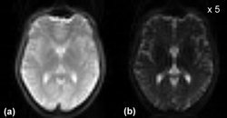
A slice of the 3D GRASE imaging volume acquired (a) without BS, (b) with BS. The intensity scale was increased by a factor of 5 for the background suppressed image.
As a result, the fractional global perfusion signal increased from 0.75 ± 0.19 (mean ± standard deviation for all subjects, expressed as percentage of the control signal) to 8.19 ± 3.14, where the increase in standard deviation is due to the within subjects variability in the degree of BS. A small reduction in perfusion signal of approximately 8% was observed with the use of BS. The BS increased the tSNR of the perfusion series by a factor of 2.4, from 3.3 ± 2.0 (mean ± standard deviation for all subjects) in the unsuppressed time series to 7.8 ± 3.2 in the background suppressed time series. Figure 3 depicts perfusion maps, showing high signal in the region of the HP. Absolute quantification of CBF values was not carried out for this study, since an accurate quantification would be precluded by the reduction in perfusion signal and the use of a short postlabeling delay.
Figure 3.
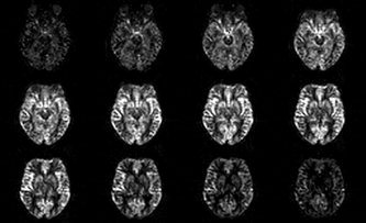
Perfusion (tag‐control) maps. Note the signal decrease in the edge slices because of the slab profile effect.
The tSNR of the control GRASE image signal and the perfusion signal in the anterior HP was not significantly different from the tSNR in the posterior region (P = 0.916 and 0.797, respectively), which indicates that the signal loss due to susceptibility artefacts is reduced by the use of the GRASE readout (see Fig. 4 and Table I). On the contrary, the tSNR of the raw EPI image signal in the anterior HP was significantly lower than the tSNR in the posterior region (for both the 3 and 2.5 mm BOLD data), which is due to signal loss caused by susceptibility effects in this area.
Figure 4.
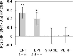
Difference in tSNR (posterior HP – anterior HP), measured in the raw EPI images (3 and 2.5 mm isotropic resolution), in the raw GRASE images, and in the perfusion images. The difference in tSNR for each subject was normalized to the mean tSNR of the whole HP. The tSNR in the posterior HP is significantly higher than the tSNR in the anterior HP in the EPI images (**P < 0.0001, *P = 0.0003).
Table I.
Signal tSNR measured in the posterior and anterior hippocampal regions, relative to the tSNR measured in the whole HP (n = 13)
| EPI (3 mm) | EPI (2.5 mm) | GRASE | PERFUSION | |
|---|---|---|---|---|
| Posterior HP tSNR | 1.075 | 1.044 | 0.981 | 0.963 |
| Anterior HP tSNR | 0.805 | 0.843 | 0.975 | 0.950 |
| Mean difference | 0.270 | 0.201 | 0.006 | 0.013 |
| Standard error | 0.035 | 0.040 | 0.050 | 0.050 |
| t‐score | 7.704 | 4.991 | 0.107 | 0.263 |
| Prob > |t| | <0.0001 | 0.0003 | 0.916 | 0.797 |
Memory Encoding Task
There was no difference in recognition scores for memory encoding during ASL and BOLD scans (F(2,24) = 0.175, P = 0.84, MS = 0.033), indicating that the order and timing of the scans did not produce any systematic effect in subjects' memory performance.
The average evoked response in the HP was higher for perfusion than BOLD (see Table II). Conversely, the tSNR per time point in this region was higher in the BOLD than in the perfusion time series. As a result, the estimated factor “effect size × tSNR per point” was similar for both techniques. However, when the number of data points in each time series was taken into account, the factor “effect size × tSNR per point × √N rep″, which is proportional to t statistics, was higher for BOLD than perfusion.
Table II.
Parameters of BOLD and perfusion signal in the HP during activation, expressed as mean ± standard deviation (n = 13)
| BOLD (3 mm) | BOLD (2.5 mm) | PERFUSION | |
|---|---|---|---|
| Effect size (%) | 0.21 ± 0.14 | 0.20 ± 0.08 | 5.87 ± 5.79 |
| HP tSNR per point | 18.3 ± 7.8 | 18.1 ± 5.7 | 0.80 ± 0.19 |
| N rep | 168 | 168 | 72 |
| Effect size × tSNR per point | 3.8 | 3.6 | 4.7 |
| Effect size × tSNR per point × √N rep | 49.8 | 46.7 | 39.8 |
The effect size was calculated as the ratio of HP activation signal amplitude to HP signal at rest. The tSNR per point was computed as the HP signal mean over the standard deviation of the time series divided by the square root of the number of time points (N rep).
At the individual level, 6 of the 13 subjects' perfusion activation maps showed significant activity in the HP (peak T values: 4.26–7.21; extent of the activation: 6.3–93.4% of the hippocampal volume). Similarly, 6 of the 13 subjects BOLD activation maps, obtained with the 3 mm BOLD data, showed significant activity in the HP with higher peak T values ranging from 5.64 to 10.67 and larger number of activated voxels, from 57.5 to 99.5% of the total voxels in the HP. The 2.5 mm BOLD data yielded activation maps with significant activity in the HP in 12 of the 13 subjects (peak Ts: 4.28–11.33; activation extent: 26.7–95%). When the BOLD time series data was truncated to match the number of points of the ASL time series, the 3 mm BOLD data showed hippocampal activation in only 4 of the 13 subjects (peak Ts: 4.68–6.49; activation extent: 19.1–92.3%) while the 2.5 mm BOLD data showed significant activity in the HP in 7 of the 13 subjects (peak T values: 4.23–6.99; extent of the activation: 5.6–93.2%) (Table III, FDR‐corrected P < 0.05, cluster > 30).
Table III.
BOLD and ASL HP activation, using a memory encoding task (FDR‐corrected P < 0.05, cluster > 30)
| BOLD (3 mm; N rep = 168) | BOLD (3 mm; N rep = 72) | BOLD(2.5 mm; N rep = 168) | BOLD (2.5 mm; N rep = 72) | ASL (4 mm; N rep = 72) | |
|---|---|---|---|---|---|
| Number of subjects with HP activation | 6 | 4 | 12 | 7 | 6 |
| Peak T range | 5.64–10.67 | 4.68–6.49 | 4.28–11.33 | 4.23–6.99 | 4.26–7.21 |
| Activation extent (% HP volume) | 57.5–99.5 | 19.1–92.3 | 26.7–95.0 | 5.6–93.2 | 6.3–93.4 |
| Group Tpeak | 4.66 | — | 7.96 | 6.19 | 6.77 |
| Group activation extent (% HP vol.) | 87.3 | — | 96.2 | 86.3 | 59.8 |
For reduced N low resolution BOLD, the activation was not significant at the group level.
When directly comparing individual t‐statistic maps (by means of a one‐way within‐subjects ANOVA), significant differences (FDR‐corrected P < 0.05, cluster size (k) > 30) were found across the groups in the HP (right HP: Fpeak = 14.49, P FDR‐corr = 0.010, k = 38; left HP: Fpeak = 13.90, P FDR‐corr = 0.010, k = 65). T‐Contrasts between conditions revealed that the BOLD high resolution activation was significantly higher than the ASL activation (right HP, Tpeak = 5.20, k = 181; left HP, Tpeak = 5.20, k = 156; FDR‐corrected P < 0.05, cluster > 30) and the BOLD low resolution activation (right HP, Tpeak = 2.22, k = 26; left HP, Tpeak = 2.18, k = 87; uncorrected P < 0.05), while no significant differences were found between the low resolution BOLD and ASL.
BOLD (Fig. 5a,b) and ASL (Fig. 5c) group maps showed activation in visual association cortex and extending forward to the HP. The ASL activation appears to be slightly more localized than the BOLD activation, which is possibly due to the different physiological parameter measured: perfusion in brain parenchyma instead of the less localized venous response, which predominantly contributes to the BOLD activation.
Figure 5.
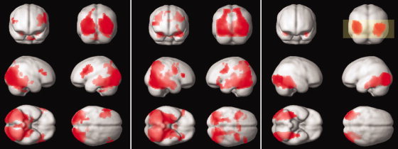
(a) BOLD 3 mm, (b) BOLD 2.5 mm, (c) perfusion activation (whole brain FDR‐corrected P < 0.05, cluster >30). The yellow box shows the coverage of the perfusion sequence.
Hippocampal activation was stronger in the group map obtained from the high‐resolution BOLD data, followed by the ASL activation and less strong for the low resolution BOLD data (Table III). The extent of the group activation in the HP was larger for the BOLD data (high and low resolution) than for the perfusion data, which activated 96.2, 87.3, and 59.8% of the HP, respectively.
DISCUSSION
Optimization of the ASL technique for perfusion‐based fMRI at high field strength yielded a sixfold increase in sensitivity with respect to previous implementations [Fernandez‐Seara et al., 2005; Wang et al., 2005]. This was achieved by improving the performance of the CASL 3D GRASE sequence with a more efficient pCASL pulse and by adding inversion pulses to suppress signal from stationary spins.
The pCASL pulse permitted the use of the body coil as transmitter and an 8‐channel phased‐array head coil as receiver, which increased the SNR of the raw images by a factor of 2. This novel labeling strategy was initially introduced by Garcia et al. [ 2005a] and implemented for this work in the Siemens platform with a slight modification of the parameters, required by the limitations in duty cycle of the body coil. Our initial experience with this pulse yielded an increase of the labeling efficiency when compared to the amplitude‐modulated control approach of 30%. Further optimization of the parameters is likely to improve this value.
The two BS pulses inversion times were chosen by taking into account sequence timing constraints and achieved a considerable degree of suppression, which resulted in increased tSNR of the perfusion series by a factor of 2.4. The second inversion time was slightly longer than the value for optimal suppression (as determined by simulations, not shown) in order to avoid uncertainty related to the polarity of the background signal. This was necessary because magnitude reconstruction of the data was performed. Alternatively, complex subtraction of tag and control raw data could be employed, which would allow maximizing the degree of suppression.
BS increased the inter‐subject variability of the fractional perfusion signal (when expressed as percentage of the control signal); however, this has no effect on the fMRI analysis of the individual subjects. Our experimental measurements also showed a small decrease in the magnitude of the perfusion signal. This is expected since, while ideal inversion pulses should not attenuate the perfusion signal, realistic pulses will slightly attenuate the signal due to pulse imperfections [Duyn et al., 2001; Garcia et al., 2005b; Ye et al., 2000]. The attenuation of the ASL signal was minimized by making one of the pulses selective to the imaging slab. This pulse, placed before the ASL pulse, should not affect the ASL signal. Thus, the attenuation of the signal is due only to the nonselective inversion pulse being used.
The optimization of the timing of the BS pulses yielded a postlabeling delay of 400 ms. While this short postlabeling delay would not be adequate if an accurate quantification of CBF was required, due to the confounding effects of transit time, it has been previously shown [Gonzalez‐At et al., 2000] that a short postlabeling delay is preferable for ASL activation imaging, since it permits to capture task‐correlated signal increases due to the increase in perfusion and the decrease in arterial transit time to the activated region. Gonzalez‐At et al. also showed that the use of a short postlabeling delay did not affect the spatial distribution of the activation. Approximate quantification of CBF would still be possible using the reference scans acquired without BS as the control signal intensity and taking into account the attenuation of the perfusion signal due to the BS pulses measured empirically.
The increase in perfusion sensitivity achieved with these modifications facilitated the use of perfusion fMRI for cognitive testing and allowed a comparison with BOLD fMRI that was performed using an established cognitive task. In spite of the ASL improvement, BOLD fMRI still yielded better within‐subject sensitivity for hippocampal activation than ASL in this study, particularly when performed using an optimized high resolution BOLD sequence. As suggested by the calculated values of effect size and tSNR obtained with both techniques, this is partly due to the increased temporal resolution of BOLD with respect to ASL, a consequence of the fact that perfusion volumes are obtained as subtraction of image pairs, which reduces the final number of data points to half the acquired raw data. Using a truncated BOLD time series, to match the number of points in the ASL time series, reduced the sensitivity of the optimized BOLD experiment to that of ASL. Approaches to speed up the ASL image acquisition have been previously reported. Turbo ASL [Wong et al., 2000] is a modification of pulsed ASL that allows the use of reduced TR by performing the control acquisition immediately after the application of the labeling pulse. Implementation of this technique for CASL is complicated due to the long duration of the labeling pulse, during which labeled blood may already enter the imaging volume. A CASL version of turbo ASL [Hernandez‐Garcia et al., 2004] has been realized by shortening the duration of the labeling pulse and TR, which allows acquisition of a larger number of time points during the same scanning period but suffers from a CNR reduction with respect to standard CASL. On the other hand, acquisition of only labeled images [Duyn et al., 2001] results in twofold improvement in temporal resolution, which would improve the sensitivity by a factor of 1.4. Although this approach may alter the special noise characteristics of perfusion fMRI conferred by the pair‐wise image subtraction, it has the potential of increasing the sensitivity of ASL to the level of BOLD.
The significant improvement in performance provided by the high resolution BOLD sequence when compared to the standard resolution BOLD sequence is partly attributable to a decrease in the effects of susceptibility induced background gradients on the BOLD signal, as demonstrated by the decrease in gradient between the tSNR of the anterior and posterior regions of the HP. However, this effect alone could not explain the improvement in sensitivity of this sequence also found in the posterior region of the HP and the visual cortex. Another likely factor contributing to the improvement in sensitivity with improved resolution is a reduction in partial volume effects that occur when nonactivating white matter present in the voxel attenuates the activation signal from the gray matter. These effects have also been observed previously in brain regions such as primary visual cortex where static susceptibility gradients are not problematic [Jesmanowicz et al., 1998]. Partial volume effects are also likely to contribute to reduced sensitivity for ASL in this study despite the lack of susceptibility artifact, considering the comparatively low spatial resolution of 4 mm isotropic for the ASL sequence used here.
At the group level, perfusion and BOLD data showed activation in visual association cortex and extending forward to the HP. The ASL activation was slightly stronger in HP than the standard resolution BOLD. This finding supports the notion that perfusion fMRI provides reduced intersubject variability than BOLD during a cognitive task, as was previously shown for sensorimotor tasks [Aguirre et al., 2002; Wang et al., 2003]. However, this advantage was no longer present when ASL group activation was compared to high resolution BOLD. The activation obtained with ASL appeared more localized than with BOLD; however, when the group activation maps were arbitrarily thresholded to produce equivalent activation volumes (data not shown), these differences were markedly reduced, suggesting that much of the observed difference is attributable to differences in sensitivity between these contrast mechanisms. Using these thresholds and considering activations within the hippocampal head, ASL yielded predominantly left lateralized activation, low resolution BOLD yielded minimal observable activation, and high resolution BOLD yielded bilaterally symmetrical activation. These findings suggest the possibility of hemispheric differences in the sensitivity of ASL and BOLD for detecting hippocampal activation during memory encoding, though the basis for these differences will need to be explored further in future work.
Two potential confounds in our experimental design cannot be addressed by our data. First, ASL and BOLD data were acquired using somewhat different block durations that were empirically chosen to match the frequency sensitivity and temporal resolution of each approach [Aguirre et al., 2002]. However, although our prior work suggests that a blocked design produces stronger activation than an event‐related design matched either for time or number of stimuli [Narayan et al., 2005], it remains conceivable that shorter task blocks somehow increase task activation when compared to longer blocks. Second, our imaging protocol used a fixed scanning order for ASL and BOLD, so a contribution of scan order effects cannot be excluded.
The results of this study offer two strategies to improve sensitivity in studies of hippocampal activation: perfusion contrast and high resolution BOLD fMRI. The ASL technique provides a reduction of signal loss and distortion due to susceptibility artifacts. These are exacerbated in the anterior HP due to its proximity to the temporal sinuses and cause significant signal loss in the BOLD images acquired using the GE‐based EPI sequence. The GRASE images have better coverage in this region, which increased the tSNR of the measurements and resulted in improved sensitivity for detecting activation. However, the ASL sequence still suffered from comparatively poor temporal and spatial resolution. The use of smaller voxels in the optimized BOLD sequence also reduced susceptibility artifacts and distortion in the hippocampal region, as well as partial volume effects, which significantly improved its performance. At present, high resolution BOLD fMRI at 3 T provides a simple approach to maximizing activation in the HP and mTL. However, improving the spatial and temporal resolution of ASL perfusion fMRI by means of higher field strength and parallel imaging techniques should allow the benefits of both approaches to be combined to produce even better sensitivity for detecting mTL activation during memory encoding.
Acknowledgements
The authors are grateful to Dr. David C. Alsop for his assistance with the implementation of the pseudo‐continuous ASL pulse.
The timing of the BS pulses was chosen after analyzing their effect on the static tissue, using a strategy similar to that proposed by [Duyn et al., 2001].
The effect of the BS pulses on the brain tissue (gray matter, white matter and CSF) was calculated as:
| (A1) |
where M z is the z component of the magnetization at the time of the imaging pulse, M 0 is the equilibrium magnetization, Ti1 is the time between the first and the second inversion pulses, Ti2 is the time between the second inversion pulse and the excitation pulse (imaging pulse), TD is the delay time, TD = TR − (Ti1 + Ti2), TR is the repetition time.
TR was set to 3.75 s due to SAR limitations. The sum of Ti1 and Ti2 was fixed as 1.6 s in order to allow for the duration of the labeling pulse and postlabeling delay. In simulations, Ti1 was varied between 1 and 1.4 s. Ti2 was then set as 1.6 − Ti1. M z was computed using Eq. (1) for CSF, gray, and white matter, assuming T1s of 4.5, 1.3, and 0.8 s, respectively.
According to this calculations, optimum suppression would be achieved for Ti1 = 1.250 s and Ti2 = 0.350 s. The final values implemented in the pulse sequence were 1.210 and 0.380 s respectively, which made the second inversion time slightly longer than the value for optimal suppression. This was necessary in order to avoid uncertainty related to the polarity of the background signal, because magnitude reconstruction of the data was performed. The suppression effect achieved in the experiments was very close to that predicted by the simulations.
REFERENCES
- Aguirre GK, Detre JA, Zarahn E, Alsop DC ( 2002): Experimental design and the relative sensitivity of BOLD and perfusion fMRI. Neuroimage 15: 488–500. [DOI] [PubMed] [Google Scholar]
- Alsop DC, Detre JA ( 1998): Multisection cerebral blood flow MR imaging with continuous arterial spin labeling. Radiology 208: 410–416. [DOI] [PubMed] [Google Scholar]
- Blinkov SM, Glezer II ( 1968): The Human Brain in Figures and Tables. A Quantitative Handbook. New York: Plenum. [Google Scholar]
- Bookheimer SY, Strojwas MH, Cohen MS, Saunders AM, Pericak‐Vance MA, Mazziotta JC, Small GW ( 2000): Patterns of brain activation in people at risk for Alzheimer's disease. N Engl J Med 343: 450–456. [DOI] [PMC free article] [PubMed] [Google Scholar]
- Brewer JB, Zhao Z, Desmond JE, Glover GH, Gabrieli JD ( 1998): Making memories: Brain activity that predicts how well visual experience will be remembered. Science 281: 1185–1187. [DOI] [PubMed] [Google Scholar]
- Cho ZH, Ro YM ( 1992): Reduction of susceptibility artifact in gradient‐echo imaging. Magn Reson Med 23: 193–200. [DOI] [PubMed] [Google Scholar]
- Chuang K‐H, Chesnick S, Koretsky AP, Talagala SL ( 2004): Optimization of the labeling time for continuous arterial spin labeling MRI. In: Proceedings of ISMRM 2004, Kyoto, Japan. p 1364.
- Constable RT ( 1995): Functional MR imaging using gradient‐echo echo‐planar imaging in the presence of large static field inhomogeneities. J Magn Reson Imaging 5: 746–752. [DOI] [PubMed] [Google Scholar]
- Detre JA, Maccotta L, King D, Alsop DC, Glosser G, D'Esposito M, Zarahn E, Aguirre GK, French JA ( 1998): Functional MRI lateralization of memory in temporal lobe epilepsy. Neurology 50: 926–932. [DOI] [PubMed] [Google Scholar]
- Detre JA, Wang J ( 2002): Technical aspects and utility of fMRI using BOLD and ASL. Clin Neurophysiol 113: 621–634. [DOI] [PubMed] [Google Scholar]
- Duyn JH, Tan CX, van Gelderen P, Yongbi MN ( 2001): High‐sensitivity single‐shot perfusion‐weighted fMRI. Magn Reson Med 46: 88–94. [DOI] [PubMed] [Google Scholar]
- Fernández‐Seara MA, Wang Z, Wang J, Rao H, Guenther M, Feinberg DA, Detre JA ( 2005): Continuous arterial spin labeling perfusion measurements using single shot 3D GRASE at 3T. Magn Reson Med 54: 1241–1247. [DOI] [PubMed] [Google Scholar]
- Frahm J, Merboldt KD, Hanicke W ( 1988): Direct FLASH MR imaging of magnetic field inhomogeneities by gradient compensation. Magn Reson Med 6: 474–480. [DOI] [PubMed] [Google Scholar]
- Fransson P, Merboldt KD, Ingvar M, Petersson KM, Frahm J ( 2001): Functional MRI with reduced susceptibility artifact: High‐resolution mapping of episodic memory encoding. Neuroreport 12: 1415–1420. [DOI] [PubMed] [Google Scholar]
- Garcia DM, de Bazelaire C, Alsop DC ( 2005a): Pseudo‐continuous flow driven adiabatic inversion for arterial spin labeling. In: Proceedings of ISMRM 2005, Miami, FL. p 37.
- Garcia DM, Duhamel G, Alsop DC ( 2005b): Efficiency of inversion pulses for background suppressed arterial spin labeling. Magn Reson Med 54: 366–372. [DOI] [PubMed] [Google Scholar]
- Gonzalez‐At JB, Alsop DC, Detre JA ( 2000): Cerebral perfusion and arterial transit time changes during task activation determined with continuous arterial spin labeling. Magn Reson Med 43: 739–746. [DOI] [PubMed] [Google Scholar]
- Gunther M, Oshio K, Feinberg DA ( 2005): Single‐shot 3D imaging techniques improve arterial spin labeling perfusion measurements. Magn Reson Med 54: 491–498. [DOI] [PubMed] [Google Scholar]
- Hernandez‐Garcia L, Lee GR, Vazquez AL, Noll DC ( 2004): Fast, pseudo‐continuous arterial spin labeling for functional imaging using a two‐coil system. Magn Reson Med 51: 577–585. [DOI] [PubMed] [Google Scholar]
- Jesmanowicz A, Bandettini PA, Hyde JS ( 1998): Single‐shot half k‐space high‐resolution gradient‐recalled EPI for fMRI at 3 Tesla. Magn Reson Med 40: 754–762. [DOI] [PubMed] [Google Scholar]
- Kim J, Whyte J, Wang J, Rao H, Tang KZ, Detre JA ( 2006): Continuous ASL perfusion fMRI investigation of higher cognition: Quantification of tonic CBF changes during sustained attention and working memory tasks. Neuroimage 31: 376–385. [DOI] [PMC free article] [PubMed] [Google Scholar]
- Maccotta L, Detre JA, Alsop DC ( 1997): The efficiency of adiabatic inversion for perfusion imaging by arterial spin labeling. [see comment]. NMR in Biomedicine 10: 216–221. [DOI] [PubMed] [Google Scholar]
- Maldjian JA, Laurienti PJ, Kraft RA, Burdette JH ( 2003): An automated method for neuroanatomic and cytoarchitectonic atlas‐based interrogation of fMRI data sets. Neuroimage 19: 1233–1239. [DOI] [PubMed] [Google Scholar]
- Milner B, Branch C, Rasmussen T ( 1962): Study of short‐term memory after intracarotid injection of sodium amytal. Trans Am Neurol Assoc 87: 224–226. [Google Scholar]
- Narayan VM, Kimberg DY, Tang KZ, Detre JA ( 2005): Experimental design for functional MRI of scene memory encoding. Epilepsy Behav 6: 242–249. [DOI] [PubMed] [Google Scholar]
- Ordidge RJ, Gorell JM, Deniau JC, Knight RA, Helpern JA ( 1994): Assessment of relative brain iron concentrations using T2‐weighted and T2*weighted MRI at 3 Tesla. Magn Reson Med 32: 335–341. [DOI] [PubMed] [Google Scholar]
- Penny WD, Holmes AP, Friston KJ ( 2003). Random effects analysis In: Frackowiak RSJ, Friston KJ, Frith C, Dolan R, Price CJ, Zeki S, Ashburner J, Penny WD, editors. Human Brain Function, 2nd ed. New York: Academic Press. [Google Scholar]
- Rabin ML, Narayan VM, Kimberg DY, Casasanto DJ, Glosser G, Tracy JI, French JA, Sperling MR, Detre JA ( 2004): Functional MRI predicts post‐surgical memory following temporal lobectomy. Brain 127(Pt 10): 2286–2298. [DOI] [PubMed] [Google Scholar]
- Squire LR ( 1992): Memory and the hippocampus: A synthesis from findings with rats, monkeys, and humans. Psychol Rev 99: 195–231. [DOI] [PubMed] [Google Scholar]
- Stark CE, Squire LR ( 2001): When zero is not zero: The problem of ambiguous baseline conditions in fMRI. Proc Natl Acad Sci USA 98: 12760–12766. [DOI] [PMC free article] [PubMed] [Google Scholar]
- Stern CE, Corkin S, Gonzalez RG, Guimaraes AR, Baker JR, Jennings PJ, Carr CA, Sugiura RM, Vedantham V, Rosen BR ( 1996): The hippocampal formation participates in novel picture encoding: Evidence from functional magnetic resonance imaging. Proc Natl Acad Sci USA 93: 8660–8665. [DOI] [PMC free article] [PubMed] [Google Scholar]
- Szaflarski JP, Holland SK, Schmithorst VJ, Dunn RS, Privitera MD ( 2004): High‐resolution functional MRI at 3T in healthy and epilepsy subjects: Hippocampal activation with picture encoding task. Epilepsy Behav 5: 244–252. [DOI] [PubMed] [Google Scholar]
- Wada J, Rasmussen T ( 1960): Intracarotid injection of sodium amytal for the lateralization of cerebral speech dominance: Experience and clinical observations. J Neurosurg 17: 266–282. [DOI] [PubMed] [Google Scholar]
- Wagner AD, Schacter DL, Rotte M, Koutstaal W, Maril A, Dale AM, Rosen BR, Buckner RL ( 1998): Building memories: Remembering and forgetting of verbal experiences as predicted by brain activity. Science 281: 1188–1191. [DOI] [PubMed] [Google Scholar]
- Wang J, Aguirre GK, Kimberg DY, Roc AC, Li L, Detre JA ( 2003): Arterial spin labeling perfusion fMRI with very low task frequency. Magn Reson Med 49: 796–802. [DOI] [PubMed] [Google Scholar]
- Wang J, Alsop DC, Li L, Listerud J, Gonzalez‐At JB, Schnall MD, Detre JA ( 2002): Comparison of quantitative perfusion imaging using arterial spin labeling at 1.5 and 4.0 Tesla. Magn Reson Med 48: 242–254. [DOI] [PubMed] [Google Scholar]
- Wang J, Zhang Y, Wolf RL, Roc AC, Alsop DC, Detre JA ( 2005): Amplitude modulated continuous arterial spin labeling perfusion MR with single coil at 3.0 Tesla. Radiology 235: 218–228. [DOI] [PubMed] [Google Scholar]
- Williams DS, Detre JA, Leigh JS, Koretsky AP ( 1992): Magnetic resonance imaging of perfusion using spin inversion of arterial water. Proc Natl Acad Sci USA 89: 212–216. [erratum appears in Proc Natl Acad Sci USA 1992;89:4220]. [DOI] [PMC free article] [PubMed] [Google Scholar]
- Wong EC, Buxton RB, Frank LR ( 1998): A theoretical and experimental comparison of continuous and pulsed arterial spin labeling techniques for quantitative perfusion imaging. Magn Reson Med 40: 348–355. [DOI] [PubMed] [Google Scholar]
- Wong EC, Luh WM, Liu TT ( 2000): Turbo ASL: Arterial spin labeling with higher SNR and temporal resolution. Magn Reson Med 44: 511–515. [DOI] [PubMed] [Google Scholar]
- Ye FQ, Frank JA, Weinberger DR, McLaughlin AC ( 2000): Noise reduction in 3D perfusion imaging by attenuating the static signal in arterial spin tagging (ASSIST). Magn Reson Med 44: 92–100. [DOI] [PubMed] [Google Scholar]
- Young IR, Cox IJ, Bryant DJ, Bydder GM ( 1988): The benefits of increasing spatial resolution as a means of reducing artifacts due to field inhomogeneities. Magn Reson Imaging 6: 585–590. [DOI] [PubMed] [Google Scholar]