Dealing with the shortcomings of spatial normalization: Multi‐subject parcellation of fMRI datasets

Abstract

The analysis of functional magnetic resonance imaging (fMRI) data recorded on several subjects resorts to the so‐called spatial normalization in a common reference space. This normalization is usually carried out on a voxel‐by‐voxel basis, assuming that after coregistration of the functional images with an anatomical template image in the Talairach reference system, a correct voxel‐based inference can be carried out across subjects. Shortcomings of such approaches are often dealt with by spatially smoothing the data to increase the overlap between subject‐specific activated regions. This procedure, however, cannot adapt to each anatomo‐functional subject configuration. We introduce a novel technique for intra‐subject parcellation based on spectral clustering that delineates homogeneous and connected regions. We also propose a hierarchical method to derive group parcels that are spatially coherent across subjects and functionally homogeneous. We show that we can obtain groups (or cliques) of parcels that well summarize inter‐subject activations. We also show that the spatial relaxation embedded in our procedure improves the sensitivity of random‐effect analysis. Hum Brain Mapp, 2005. © 2005 Wiley‐Liss, Inc.

INTRODUCTION

The use of brain imaging to probe for the relation between function and structure in the human brain relies on our ability to study groups of subjects. One of the fundamental difficulties in the process of extracting knowledge across subjects lies in the inter‐individual variability. The most common solution to this problem, which has been very useful, has been to spatially normalize the anatomical and functional data in a common reference space. Usually, this space is chosen to approximately match the Talairach space [Talairach and Tournoux,1988], and results are reported in the Talairach coordinate system (x, y, and z, in mm). The actual resolution of the resulting group analysis is clearly not at the voxel level, however, due to the normalization procedure shortcomings and further spatial filtering. It therefore turns out that the same Talairach coordinates may correspond to different brain structures across individuals. In addition, data queries usually refer to regions of interest (e.g., “Is the Broca area activated?”) and not to specific x‐, y‐, and z‐coordinates. In this respect, the stereotactic normalization procedure is not optimal. Here, we develop the rationale leading to a new approach.

Some Limitations of Spatial Stereotactic Normalization

Neuroimaging studies often comprise 10–20 subjects who undergo the same experimental paradigm. For each subject, both anatomical and functional images are recorded, coregistered, and assumed to be in the same space. The anatomical images are then normalized to a standard template and the computed transformations are then applied to normalize functional datasets. Statistical analysis can then be carried out on a voxel‐by‐voxel basis. Fixed or random‐effects analyses are used to assess the presence of an effect within the group, taking second‐level (i.e., inter‐subject) variability into account or not. Although computationally efficient, this procedure relies on the estimation of a geometric transformation between each dataset and a template image (normalization; see Ashburner and Friston [1999] for a typical method), and a correct registration between anatomical and functional volumes. The results of this spatial normalization are not easy to validate for complex 3‐D objects such as brain structures, and more generally raise the following questions or remarks.

Does any perfect correspondence exist between a given anatomical image and a template? Studies of anatomical variability across subjects such as sulcogyral [Rivière et al.,2002] and cytoarchitectonic [Roland et al.,1997] suggest a negative answer in general.

Even if such a correspondence does exist, how do we validate the procedure and measure the accuracy of the transformation estimate? When measured approximately, the residual variability is of the order of several millimeters [Collins et al.,1998; Hellier et al.,2003].

Assuming that the anatomy is perfectly registered with the template, how accurate is the correspondence with functional data? Given the coarse precision and the distortions of echo‐planar imaging (EPI), a precision of less than one or two voxels (5–10 mm) is difficult to guarantee. The correspondence is also blurred by partial volume effects.

Assuming that the anatomy is coregistered with functional data, how much functional variability exists between subjects due to genetic or epigenetic factors? Although this variability is difficult to formally evaluate, it is likely to be again of the order of centimeters [e.g., see Wei et al.,2004] or even more in situations where the functional organization differs across subjects.

These issues, illustrated for example in Nieto‐Castanon et al. [2003] and Brett et al. [2002], have long been known, and a classic approach to address them has been to sacrifice the spatial resolution of fMRI datasets to gain robustness against misregistrations. In image‐processing terms, this can be viewed as spatial low‐pass filtering (smoothing) and undersampling (reduction of the number of spatial degrees of freedom). It thus is not unusual to apply 10 mm (full‐width half‐maximum [FWHM]) or more spatial smoothing of functional magnetic resonance imaging (fMRI) datasets before carrying out group analyses. This usual isotropic Gaussian smoothing is not optimal for neuroscientific inference, because it does not necessarily fit the underlying anatomical or functional brain structure. Moreover, this technique assumes that all spatial differences across subjects are irrelevant, although some of them may reflect intrinsic anatomo‐functional differences. Below, we propose to adapt the resolution of functional images inter‐subject analysis.

Parcellation: An Adapted Reduction of the Image Resolution

A possible way to overcome the shortcomings of spatial normalization is to introduce prior anatomical information in the undersampling of the data. For instance, smoothing can be carried out along the cortex [Andrade et al.,2001; Dale and Sereno,1993; Fischl et al.,1999; Sereno et al.,1994] to account for the structure of the gray–white matter interface. Another approach developed by Kiebel et al. [2000] uses anatomical basis functions to group voxels. Both these works are limited when dealing with multiple subjects.

Recently, Flandin et al. [2003] proposed to group voxels into anatomically and functionally homogeneous parcels across subjects. This latter approach is appealing for several reasons (1) the voxels, which are the spatial units of functional images, define an arbitrary spatial resolution, and small regions modeled as groups of voxels may better reflect true regions of activity as they can be characterized in fMRI; (2) this makes the analysis less sensitive to artifactual or intrinsic misregistrations in multi‐subject studies; (3) technically, this undersampling of the brain volume or surface reduces the well‐known problem of multiple comparisons, allowing for less conservative Bonferroni corrections; and (4) in general, it may also better take into account the true between‐subject anatomical variability such as cytoarchitectonic [Roland et al.,1997] or sulcogyral [Rivière et al.,2002] structure of the cortex. The work proposed here follows this parcellation idea.

Previous Work Related to Parcellation

Although the idea of constructing automatically anatomo‐functional parcels is relatively recent in neuroimaging, some works are clearly related to this line of thought and we briefly review some of those attempts.

First, brain parcellations have been proposed in a purely anatomical context. Existing methods are based either on prior knowledge of anatomy and connectivity [Meyer et al.,1999], on sulcal geometry [Lohmann and von Cramon,2000; Mangin et al.,1995; Tao et al.,2001; Thompson et al.,1996], on sulcal identification [Cachia et al.,2003], or on probabilistic atlases [Fischl et al.,2004; Sandor and Leahy,1997]. These parcellations can be used in a functional context, after coregistration of anatomical and functional images. This may be done semiautomatically [Nieto‐Castanon et al.,2003] or using atlases [Tzourio‐Mazoyer et al.,2002]. This procedure might suffer from poor anatomo‐functional correspondence related to EPI distortions; more generally the functional homogeneity of the resulting parcels should be checked for inference purposes. By contrast, parcellation based on functional information is a relatively novel approach, with specific challenges.

Clustering of similar time series yields homogeneous functional regions [Simon et al.,2004], but purely functional clusters are well defined only locally [Grill‐Spector et al.,2004] and specific methods have to be designed for the parcellation of the entire brain. For instance, Penny and Friston [2003] have proposed an expectation maximization (EM) algorithm to jointly model the spatial location of activation, together with the activation amplitude at each cluster. This joint modeling is reminiscent of Flandin et al. [2002b]. This model is rather adapted to encode sparse activation patterns, however, whereas we aim at a parcellation of the entire brain volume or large brain regions consistently across subjects.

Flandin et al. [2002a,b,2003] launched fMRI‐tailored parcellation approaches; they have proposed a clustering approach based on Gaussian mixture models (GMMs) that group voxels from multiple datasets according to a spatio‐functional criterion and blindly to the subject. This is a very effective approach, because it is based on quick algorithms. In this framework, the anatomy of the subject can be introduced adequately in the core algorithms and the technique naturally yields results such that inter‐subject analysis assumptions are naturally enforced. To our knowledge, this is a first approach to deal with anatomical and functional variability for multi‐subject analysis; however, it has a few limitations. First, it does not guarantee the spatial connectivity of the parcels. Second, it does not necessarily produce multi‐subject parcels (or cliques) in which each subject of the group is present, which should be a desirable feature. 1 This may or may not be a limitation depending on whether subjects are functionally homogeneous or not, but some applications may require that corresponding parcels can be found in all or most of the subjects. Last, the definition of a spatio‐temporal criterion may be cumbersome, because it contains nonhomogeneous terms and the relative weighting of the functional and the spatial information remains an open question.

Desired Characteristics of Brain Anatomo‐Functional Parcellation

In this section, we briefly describe the desired parcel characteristics.

First, on an intra‐subject basis, parcels should be spatially connected so that they can represent homogeneous anatomo/functional regions of individual subjects.

Second, still on an intra‐subject basis, parcels should be functionally homogeneous. This could be achieved, for instance, by requiring that voxels belonging to a common parcel have similar time courses or that they have homogeneous activity summarized by model parameters.

Third, on an inter‐subject basis, it seems reasonable to require that the voxels of a given parcel should be close in Talairach space. For instance, they should lie less than 10 mm apart from each other. Moreover, the warp implied by parcel correspondences should be smooth, i.e., neighboring parcels of one subject should be associated with neighboring parcels of another subject.

Fourth, inter‐subject cliques should also be homogeneous in the functional domain. However, it would clearly not be reasonable to require that their time courses be similar to each other because of physiological activity or condition timing that may not be necessarily reproducible from subject to subject. We therefore require that subject parcels have similar effects for a contrast of conditions or a group of contrasts of interest.

We propose a parcellation method that addresses all the aforementioned issues. More specifically, we first solve the intra‐subject parcellation problem by introducing a method that enhances the functional homogeneity of the parcels while keeping them connected. As the inter‐subject problem is more complex, we solve it in a hierarchical fashion: we first find clique prototypes that summarize the essential characteristics of the multi‐subject dataset, then we derive subject‐specific instances of the clique prototypes. With this step, we guarantee that each clique will be represented by at least one voxel in each subject (onto property) and make sure that the spatial structure of the parcellation is the same across subjects (spatial regularity). These correspondences are also constrained in Talairach space. We then proceed with the parcellation in each subject, which preserves the prototype topological structure.

Intra‐ and Inter‐Subject Parcellation Techniques

We here propose an alternative to the original approach by Flandin et al. [2003]. This alternative is based on two contributions. First, we consider the problem of parcelling each subject's dataset, in which we optimize functional homogeneity of the parcels while preserving the spatial connectivity structure. For this issue, we derive a spectral clustering algorithm for fMRI data. Second, we introduce a method that carries out inter‐subject parcellation by searching analogous regions across subjects; analogous regions are defined from their functional activity and their global topographic structure. The key point here is that these constraints are first enforced on a set of anchor points (the prototypes) and propagated to all of the dataset using the intra‐subject procedure. In the following, parcel denotes the intra‐subject set of voxels whereas clique makes reference to an inter‐subject group of parcels.

The method is tested on an experimental protocol carried out on 31 normal subjects. The experimental data was acquired while subjects were presented various stimuli and involved in several different tasks (10 experimental conditions). With this paradigm, functional homogeneity of the parcels can be characterized from many contrasts of experimental conditions.

We first describe our two‐step parcellation procedure and the dataset that is used in our experiments. We then turn to our main application, which is parcel‐based random‐effect (PRFX) analysis, and we describe the parcels and cliques obtained with our dataset. We also compare the PRFX maps with those obtained with standard random‐effects (RFX) analysis. Last, we discuss the techniques used in the present work as well as the underlying model of fMRI datasets, and the limitations of our parcellation approach. The algorithmic and implementation details of our method are detailed in the Appendix.

MATERIALS AND METHODS

We used an event‐related experimental paradigm consisting of 10 conditions. Subjects underwent a series of stimuli or were engaged in tasks such as passive viewing of horizontal or a vertical checkerboards, left or right click after audio or video instruction, computation (subtraction) after video or audio instruction, and sentence presentation from audio or visual modality.

Events occurred randomly in time (mean interstimulus interval of 3 s), with 10 occurrences per event type (except motor button clicks for which there were only 5 trials per session).

Thirty‐one right‐handed subjects participated in the study. The subjects gave informed consent and the protocol was approved by local ethics committee. Functional images were acquired on a 3T Bruker (Germany) scanner using an EPI sequence (repetition time [TR] = 2,400 ms, echo time [TE] = 60 ms, matrix size = 64 × 64, and field of view [FOV] = 24 cm × 24 cm). Each volume consisted of n _a 4‐mm‐thick axial slices without gap, where n _a varied from 26 to 40 according to the session. A session comprised 130 scans. The first four functional scans were discarded to allow the MR signal to reach steady state. Anatomical T1 images were acquired on the same scanner, with a spatial resolution of 1 × 1 × 1.2 mm³.

Functional MRI data processing consisted of: (1) phase map distortion correction (when available, on seven subjects); (2) temporal Fourier interpolation to correct for between‐slice timing; (3) motion estimation (for all subjects, motion estimates were smaller than 1 mm and 1 degree so that no correction was carried out on the datasets); and 4) spatial normalization of the functional images and re‐interpolation to 3 × 3 × 3 mm³. This preprocessing was carried out with the SPM2 software [e.g., see Ashburner et al.,2004].

Datasets were also analyzed using the SPM2 software, using standard high‐pass filtering and autoregressive (AR)(1) whitening. For further analysis, only the effect (or general linear model [GLM] parameters) magnitude of each voxel for each condition was retained. We determined a global brain mask for the group by considering the voxels within at least half of the individual brain masks defined with SPM2. It comprises approximately 55,000 voxels.

Intra‐Subject Parcellation

Let us assume that we want to reduce spatial resolution of the data from V voxels to Q parcels (e.g., Q = 1,000) for a given subject. We carry out a parcellation procedure that attempts to group voxels that have close functional profiles with the constraint that the resulting parcels contain connected voxels only. To achieve this, we model the set of voxels as a graph whose vertices are the voxels and whose edges link neighboring voxels such that the topology of the graph codes the spatial structure of the dataset. Next, each edge next is given a length that reflects the difference of the functional information carried by the voxel‐based time courses. Let

(1)

be a GLM of one dataset, where Y is the (T × V) data matrix, X the T × d design matrix, β is the d × V matrix of the model parameters, and η the residual noise T × V matrix. The parameters characterize the functional properties of the voxels. The covariance matrix of the parameter estimates Λ is computed according to the specification of the design matrix, taking into account the particular temporal preprocessing used for estimating the parameters [Ashburner et al.,2004]. If v and w are neighboring voxels, with parameters β(v) and β(w), the value associated with the edge (vw) will be

(2)

The lengths of the graph edges thus code functional dissimilarity between neighboring voxels.

The local distances between neighboring vertices can then be integrated along paths of the graph G to yield global distances. This is typically done using Dijkstra's [1959] algorithm. These global distances δ_G(v,w) reflect both the functional and spatial structure, i.e., the topology of the dataset. Δ_G =(δ_G(v, w))_v,w∈V×V is a huge (V × V) matrix. But, using geometrical arguments, one can show that it can be reduced to an N × k, k << N matrix E without discarding much information. E can be thought of as a data‐tailored coordinate system and should minimize the following distortion function:

(3)

where the sum is computed over all the pairs of vertices of the graph. The minimization of 𝒟 can be obtained exactly given the distance matrix Δ_G. This minimization yields a multidimensional scaling (MDS) representation of the dataset; it is an arbitrary coordinate system that captures most of the information of interest Δ_G. The dimension k of the embedding (coordinate system) E is k = 3, because Δ_G essentially models a 3D graph (see Appendix A for more details and interpretation). Last, intra‐subject parcels can be derived by a simple C‐means clustering of E. For inter‐subject parcellation, however, it is more interesting to build the final clusters in a way that is consistent across subjects. The global setting that includes computation of the distances on the graph G and MDS is known in the literature as the Isomap algorithm [Tenenbaum et al.,2000]. The association of Isomap and clustering is known as spectral clustering. An illustration is given on a toy example in Figure 1.

Figure 1.

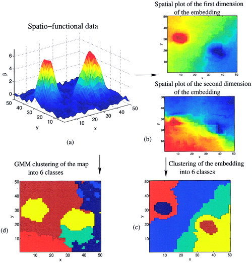
Spectral clustering procedure. a: Input dataset that consists of pixels on a (x, y) grid, endowed with a functional information β. b: Through Isomap, an embedding E = (e ₁, e ₂) of the dataset is derived; the components e ₁, e ₂ can be represented and color‐coded as spatial maps. c: A simple C‐means clustering is then applied to the dataset. This clustering separates the two peaks, and partitions the (x, y) grid into connected and homogeneous regions. It mainly reflects the relative position of the pixels with respect to the two peaks. By contrast, direct Gaussian mixture model (GMM) clustering of the (x, y, β) coordinates (d) yields unconnected clusters; in particular, it gathers the two peaks in a single component.

We show in Appendix B that such a procedure produces parcels that are functionally more homogeneous in average than parcels defined in the Talairach coordinate system. Moreover, the resulting parcels are spatially connected.

Inter‐Subject Parcel Building

The embeddings defined in equation (3) are extremely useful for intra‐subject parcellation, but they cannot be extended simply across subjects. To fulfill the criteria defined above, our strategy consists of the following: (1) finding clique prototypes defined at the population level, where a prototype is characterized by Talairach coordinates and a functional profile; (2) identifying subject‐based instances of these prototypes, where the instances should be close to the clique prototypes in Talairach space, functionally similar, and have a globally similar spatial layout; and (3) defining intra‐subject parcels given the prototypes of the given subject. This issue is solved using our intra‐subject parcellation scheme, which is designed to maximize the functional similarity while preserving the topology of the prototypes. This hierarchical strategy readily results in a three‐step method.

First, clique prototypes are derived by a C‐means clustering algorithm of the functional profile β(.) of the voxels of the pooled (multi‐subject) datasets. More specifically, this clustering procedure is spatially constrained: voxels can only be assigned to prototypes that are less than a predefined distance d _τ apart in Talairach space, so that each prototype represents the functional activity locally. The exact algorithm is described in Appendix C. After convergence, the voxels‐to‐prototypes assignments are discarded, because they do not meet the spatial regularity/onto property constraints defined above. Only the clique prototypes, i.e., Talairach coordinates τ(c) and functional profile β(c) for each clique c are kept.

Second, in each subject s ∈ [1 … S], and for each clique c, a prototype p(c,s) is derived. It is a voxel in dataset s that best corresponds to the clique prototype. As mentioned previously, the prototype with functional profile β(p) and Talairach coordinates τ(p)− should minimize functional dissimilarity while being close in Talairach space. Moreover, the warp w_s: τ(c) → τ(p(c, s)) should be regular ∀s ∈ [1 … S]; hence we require the Jacobian of w _s to be positive everywhere. The details of this step discussed in Appendix D.

Third, in each subject s ∈ [1 … S], the voxels can now be assigned to parcels. This is simply carried out by considering the embedding E defined in equation (3) and assigning each voxel to the nearest prototype p in the E space. As detailed in Appendix B, this procedure enhances the intra‐parcel homogeneity while preserving the topology of the subject‐based prototypes, which, given the second step, respects the topology of the clique prototypes.

This procedure is summarized in Figure 2. We have observed a reduction of the average intra‐clique functional variance by 6% using this functional parcellation technique with respect to a procedure that does not take functional information into account.

Figure 2.

Inter‐subject hierarchical parcellation procedure. The definition of inter‐subject parcels consists of three steps: (1) definition of the clique prototypes, based on functional data clustering and constrained by Talairach coordinates; (2) definition of subject‐based instances of the clique prototypes, such that the corresponding warp is spatially regular; and (3) intra‐subject assignment of the voxels‐to‐subject defined parcels by nearest‐prototype assignment in the E coordinate system (see equation [3]).

Using Parcellation to Carry Out RFX Analyses

Once the final assignment from voxels to parcels is computed, one can handle parcels within a clique as voxels at the same coordinate position in a standard multi‐subject analysis. Given a contrast of interest c and a clique q, the average contrast values are given by e(s,q) = c ^T (s,q), where (s, q) denotes the average value of the estimated effects of all the voxels that belong to clique q, for a given subject s ∈ 1. S.

The standard RFX test then reads:

(4)

Under the null hypothesis, T(q) has a Student distribution with (S − 1) degrees of freedom, as in standard random effect tests.

One can notice that this test is valid only if there is actually one parcel of each subject in each clique, which is why the onto property is required in the inter‐subject parcellation, and the resulting T(q) maps are defined on Q cliques, with Q being mostly smaller than the number of voxels in any dataset. This means that the multiple comparison problem in the statistical assessment is alleviated with respect to traditional voxel‐based analyses.

One might expect that under the null hypothesis, the value given by equation (4) does not conform itself to the Student distribution. To check the false positive control (type I risk of error) of the parcel‐based RFX (PRFX) test, we carried out simulations on noise‐only data: We drew voxel‐based parameter β(v) map from a multivariate centered normal distribution and computed an associated inter‐subject parcellation based on the 10 parameters defined at each voxel. PRFX tests were then been carried out on the same contrasts as for the real data. The empirical distribution of the P‐values derived from the assumed Student distribution can be compared to their distribution under the null hypothesis, which should be uniform on the [0,1] interval. This comparison, presented as a probability plot, illustrates and quantifies the deviation from the null hypothesis of the t statistics in noise‐only data.

We next repeated the same experiment, but the parcellation was computed using a contrast of the voxel‐based estimated parameter c ^T (v), and the same contrast was tested in the PRFX analysis.

To check that the proposed method indeed controls for the type I error rate, we generated non‐parametrically null distributions of the statistic in equation (4) by sign swap of all the global functional information randomly across subjects, and recomputed the parcellation and derivation of the PRFX test. This time‐consuming procedure enables to have an unbiased control on the false positive rate on real data.

RESULTS

The parcellation analysis was carried out on the 31‐subject group. As detailed above, Q = 10³ inter‐subject cliques were derived. The cut‐off distance for voxel‐to‐prototype (step 1) or clique prototype‐to‐parcel prototype (step 2) was chosen as d _τ = 10 mm.

Preliminary Study of Spatial Variability

To illustrate the behavior of the parcellation algorithm, we first present the spatial organization of the parcels in the clique that was most sensitive to the (left click‐right click) contrast. Figure 3 (top) shows a coronal view in radiological convention of the image that represents the empirical frequency of this clique across subjects overlaid on an anatomical template. The same frequency overlaid on a standard model of the gray–white matter interface is depicted in Figure 3 (bottom). No voxel was included more than 25 times in the clique across subjects, although the clique was actually represented in all 31 subjects. The average distance between any two centers was 6 mm.

Figure 3.

Empirical frequency across subjects of the clique that responds most to the left click‐right click contrast. Top: A coronal view, superimposed on an anatomical template. Bottom: In 3D, superimposed on a standard gray–white matter interface. The color bar codes the actual frequency of the clique at the given voxel, the maximal frequency being 25 subjects (over 31).

RFX Maps: Sensitivity

Activation maps obtained at the clique level were compared to those maps obtained from a voxel‐based analysis carried out on the same dataset. The voxel‐based maps were derived after a 5‐ or 12‐mm smoothing on the functional data. All maps were z‐transformed and thresholded either at the P‐value of 10⁻³, uncorrected for multiple comparisons (z = 3.09), or at the P‐value of 0.05, corrected for multiple comparisons. The multiple correction procedure is the standard Bonferroni. The thresholds resulting from the Gaussian random field theory are as severe as Bonferroni thresholds are, even on the smoothed data. All the images are displayed on the group‐average T1 image. The spatial localization of the cliques is defined as follows: in the template space, the group‐average centers of the cliques are computed and a Voronoi parcellation is carried out, i.e., each voxel in the template space is assigned to the closest clique center.

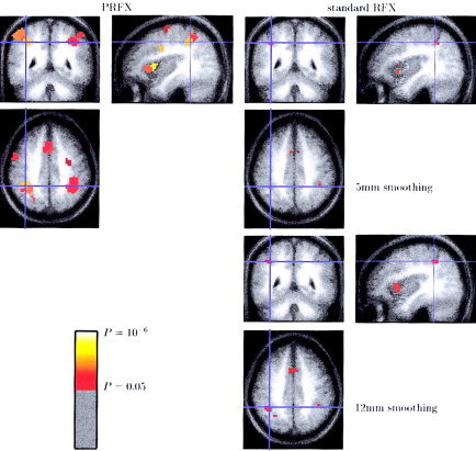
In Figure 4, we present maps of the PRFX and RFX tests for the (left click‐right click) contrast, corrected and uncorrected for multiple comparisons.

Figure 4.

Random‐effects maps for the left click‐right click contrast. Top left: On the parcelled dataset, without correction for multiple comparisons. Top right: On the original dataset (5‐mm smoothing), without correction for multiple comparisons. Bottom left: On the parcelled dataset, after correction for multiple comparisons. Bottom right: On the original dataset (5‐mm smoothing), without correction for multiple comparisons. We use radiological conventions; the color scale is the same on the left and right sides.

Figure 4 illustrates the results of the PRFX compared to the results of the standard RFX analyses. It can be observed that the PRFX results show in general a greater sensitivity than the RFX results did after 5‐mm smoothing. The locations of the activation foci are mostly comparable. When correcting for multiple comparisons, the sensitivity of the PRFX procedure becomes much greater than that of the standard analysis. The same behavior has been found for the other contrasts that we studied (right click‐left click, video sentences–audio sentences, audio sentences–video sentences, and computation–reading).

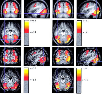
In Figure 5, we present maps for the PRFX and RFX after 5‐mm smoothing, and RFX after 12‐mm smoothing tests for the computation‐reading contrast, at the corrected P‐level.

Figure 5.

Random‐effects maps for the computation‐listening/reading sentences contrast. Top left: On the parcelled dataset. Top right: On the original dataset, after 5‐mm smoothing. Bottom right: On the original dataset, after 12‐mm smoothing. The thresholds are chosen at the Bonferroni corrected level (on the smoothed data, we tried with thresholds inspired from the Gaussian random field theory, but they were at least as severe).

Figure 5 shows that after stronger smoothing (12‐mm FWHM instead of 5‐mm), the sensitivity is partly recovered in the standard RFX map but remains less than that in the PRFX. The thresholds resulting from the Gaussian random field theory are as severe as Bonferroni thresholds are, even on the smoothed data.

PRFX Maps: Localization

An important feature of the parcellation‐based analysis is that the results can be presented in the anatomical referential of any of the subjects. We illustrate this in Figure 6 that shows the spatial map of the video sentences‐audio sentences contrast at both the group and subject level. More precisely, we show for this contrast the smoothed (12‐mm) RFX map, the PRFX map represented in the average group coordinates, the PRFX map represented in the anatomical space of Subject 2, and the intra‐subject z‐map for the same contrast and same subject.

Figure 6.

Spatial map of the video sentences‐audio sentences contrast at the group/subject level. Top left: Smoothed (12‐mm) random‐effects map for the contrast. Top right: Parcel‐based random‐effect map for the contrast, represented in the average group coordinates. Bottom right: Parcel‐based random effect map for the contrast, represented in the anatomical space of one subject. Bottom left: Intra‐subject z‐map for the same contrast, same subject. The random‐effects maps are thresholded at the P = 10⁻³ uncorrected level; the intra subject z‐map is thresholded at a lower level (P = 10⁻²) to ease the comparison. The parcel‐based random‐effect model yields intermediate representations between coarse group activations and subject‐specific activations.

Although the smoothed RFX map and the intra‐subject activation map show quite different local maxima positions, group and individual PRFX maps are more consistent: The PRFX map in the group referential shows activations that are clearly more posterior than those in the smoothed RFX map, and the PRFX map in the subject referential clearly warps the group activation parcels toward the more focal subject activations. This effect is quite large: the distance between the local maxima of the smoothed RFX map and the intra‐subject maximum is more than 20 mm, and the subject has no activation at the coordinates of the local maximum of the smooth RFX map. Parcellation‐based analysis facilitates the comparison between the individual and the group maps. In the present case, it can disambiguate the identification of word‐sensitive regions from other specialized regions of the ventral visual cortex.

PRFX Maps: Specificity

Using the intra‐subject parcellation of the actual dataset, we generated null datasets by drawing random effects β(v) for each voxel in a normal distribution. The inter‐subject hierarchical parcellation procedure was then carried out using the simulated values of β for the 10 conditions. The PRFX test was finally carried out on the ensuing cliques. In doing so, we checked that carrying out the parcellation and RFX test on the same data did not increase the risk of false positive in the resulting statistic. For each contrast tested in our experiment, 10⁵ simulated datasets were generated and tested. Deviation of the distribution of these samples from the null hypothesis was assessed by plotting the P‐values obtained through the theoretical Student distribution model against their rank (probability plot). The case probability plot for the left click‐right click contrast is given in Figure 7. It demonstrates that there is a slight deviation from the null hypothesis, but the analytical probability is higher than is the empirical rank. This means that the Student test is rather conservative and can be used safely. Note that the same behavior can be seen when using other contrasts. This experiment was carried out on 10 subjects.

Figure 7.

Probability plot of the statistical results obtained from null dataset. This Figure compares the empirical P‐value obtained from the data with the theoretical P‐value. If there was no bias in the distribution, all the points should lie on the diagonal. The probability plot is above the diagonal, showing a measured statistic that is lower than the expected one.

Our second kind of simulation consisted of parcelling and testing using the same contrast. In the second case, we obtained no bias in the distribution (data not shown).

Moreover, we carried out a data‐tailored estimation of the P = 0.05 corrected threshold using nonparametric group analysis [Nichols and Holmes,2002]: we generated a null distribution of the effects by random sign swap of the subject parameters. The inter‐subject parcels were then recomputed for each dataset and the PRFX statistic was derived. The maximum of the map was kept for each of the aforementioned contrasts, with the experiment being carried out 10³ times. This yielded an empirical distribution of the maximum PRFX statistic under the hypothesis that the mean effect was null across subjects. We then used this empirical distribution to carry out corrected tests. In Table I, we compare the theoretical and the empirical thresholds, as well as the number of supra‐threshold parcels, for all aforementioned contrasts.

Table I.

Comparison of the empirical z threshold derived empirically by sign swap of the functional information, parcellation, and PRFX test, with the analytical theoretical threshold

Contrast	L–R click	R–L click	Video–audio	Audio–video	Computation–sentences
Theoretical threshold	3.89	3.89	3.89	3.89	3.89
Suprathreshold parcels	11	8	88	77	40
Empirical threshold	3.59	3.84	4.17	4.14	3.79
Suprathreshold parcels	14	10	78	67	47

In each case, we also give the number of suprathreshold parcels. Note that the sensitivity is equivalent. L, left; R, right.

Clearly, the specificity of the nonparametric test is very similar to the specificity of the parametric test, and the effect of the method on the number of supra‐threshold parcels is mild.

Implementation issues and CPU Time

The algorithms presented have been implemented partly in MATLAB (The MathWorks, Natick, MA) and partly in C, using C‐MEX binding, for the sake of computation speed. On a 3 GHz P4 PC, the computation of each intra‐subject parcel took a couple of minutes, and the inter‐subject parcel grouping after precomputation of the intra‐subject embedding‐ took 10 min; these times scale linearly with the number of subjects and parcels. The design of the method allows addressing the issue of dealing with large databases of subjects. If a large collection of parcelled brains is already available, it is possible to simply increment it using existing clique prototypes and steps 2 and 3 defined above. Altogether, the procedure lasts 65 min for a 31‐subject dataset and 10³ cliques. This is more time than that required with standard multi‐subject analysis, but it can still be acheived fairly easily.

DISCUSSION

On the Parcellation Methods

Whereas standard group analysis implicitly require a voxel‐by‐voxel match between subjects, we suggest here an alternative framework allowing for a more flexible treatment of the spatial aspects of inter‐subject averaging. We presented a multi‐subject parcellation technique inspired by previous work by Flandin et al. [2003]. With respect to this previous work, we chose to carry out the clustering on the functional data such that parcels would necessarily be spatially connected clusters of voxels. Moreover, the inter‐subject parcel‐matching algorithm was designed to enforce the constraint that all subjects are represented in a clique (an inter‐subject group of parcels) with consistent across‐subject topographies. A potential alternative to our intra‐subject parcellation procedure is the use of agglomerative clustering, as proposed in Almeida and Ledberg [2001]. Our experience on this matter, however, is that agglomerative clustering algorithms do not perform well for irregularly sampled data such that some regions would tend to be oversegmented whereas others may be unnecessarily merged. Moreover, these algorithms are known to be sensitive to noise and outliers [Stanberry et al.,2003]. By contrast, the spectral clustering algorithm used here (detailed in Appendix A) allows for a more regular sampling of the brain volume.

Our algorithm is not quantitatively directly comparable to voxel‐based spatial normalization techniques [e.g., see Ashburner and Friston,1999; Collins and Evans,1997; Woods et al.,1998], or to more sophisticated landmark‐based and surface‐based coregistration techniques [Fischl et al.,1999; Liu et al.,2004]. It is assumed here that a first normalization step has been applied to the input data, and the method is designed to deal with residual spatial variability that is not easily dealt with and can be of a different nature than anatomical variability, i.e., functional variability. Moreover, obtaining better correspondences across subjects is not equivalent to improving normalization, which assumes a generic template.

Importantly, parcel‐based analysis of an fMRI dataset is fully compatible with a systematic reporting of individual and group activations in Talairach space, the constitution of large databases, and meta‐analysis in Talairach space.

Results of Parcellation and the PRFX Procedure

By relaxing the spatial constraint of current random‐effects analysis, we have shown that a large increase of sensitivity can be obtained in inter‐subject studies. This was not at the expense of a greater risk of false positive. The procedure should also provide a better estimate of the activity location than voxel‐based methods, because the results have a subject‐per‐subject representation that probably yields a better anatomo‐functional correspondence. We discuss below some of the results. One should first notice that this procedure is always feasible, however, and that it systematically provides an inter‐subject parcellation that meets all the criteria that we have detailed previously.

Spatial Variability of Parcels Within a Clique

Figure 3 shows the variability of the parcels of a given clique in Talairach space. The proposed algorithms simply impose that parcel centers of mass should lie within a 10‐mm ball around the clique center in Talairach space. Although 10 mm may seem a large distance, it may well reflect the overall spatial uncertainty due to factors such as registration of individual anatomy with a Talairach template, the non‐affine deformations between EPI sequences and anatomical images, and simply anatomo‐functional variability. Nevertheless, it may well be that some cliques contain parcels located in different brain structures. As discussed below, this could be avoided, for example, by using high‐level anatomical information from the macroscopic anatomical brain structure (gyri, basal ganglia, etc.).

For a clique of interest, the variability of the parcel centers has been estimated to 6 mm; however, the spatial regularization imposed in the inter‐subject parceling procedure may have artificially reduced this variability. Moreover, we found that the voxels of the corresponding parcels did not overlap completely: at most, we found an overlap between 25 subjects among 31 that had a parcel in the clique (see Fig. 3). Despite the mild variability of the parcel centers, the intersection of the 31 parcels is therefore empty. This explains why small spatial relaxation should benefit to sensitivity.

Random‐Effects Maps

The maps presented in Figure 4 show that the PRFX maps have supra‐threshold locations comparable to those obtained with conventional RFX analyses. The sensitivity is improved, however, resulting in higher statistics in activated areas and thus sharper contrast in the z‐maps, which results in lower P‐values. Furthermore, the effect is even stronger when considering statistical thresholds corrected for multiple comparisons, because parcellation reduces the effect of Bonferroni correction.

As shown in Figure 5, using smoother (12‐mm FWHM instead of 5‐mm) maps in RFX analysis, one can partly recover the sensitivity of the RFX test, but the peak activation significance remains lower than that for the PRFX for all the contrasts that we studied, especially after correction for multiple comparisons. The choice of a 5‐mm smoothing may seem unfavorable to the traditional RFX maps; however, this corresponds to a number of resolution elements (RESELS) per subject close to the number Q of parcels. For comparison, 8‐mm smoothing reduces the number of RESELS down to approximately 270. Our parcels, however, were comparable in size to balls with a 6‐mm radius. The question of the comparison of the number of parcels and the number of RESELS has been discussed more thoroughly in Flandin et al. [2002a]. Whatever the precise correspondence between smoothing width and parcel number, one may consider that intensive smoothing undermines the interpretation of the spatial extent of activations, worsens partial volume effects, and may in some configurations decrease sensitivity.

We next emphasize that group studies should not be limited to reporting group activation maxima after a wide smoothing of the individual maps. This is clear from Figure 6, where the smooth RFX map differs considerably from the activation map of one of the subjects, this subject being neither an outlier nor an exception. By contrast, the PRFX map gives at the group level a possibly more realistic picture of the activation topography and provides a build‐in warp of this topography into the referential of each subject. This simple observation could be the starting point for a novel approach to group studies.

Importantly, there do not seem to be spuriously activated regions for the contrasts studied. Indeed, one could have thought that grouping regions with similar functional profile may have inflated the number of false positives. This is seemingly not the case here. This point is discussed more thoroughly below.

Potential Bias in RFX Statistics?

The control of false positive activation is an important concern in any inferential method, and therefore for the PRFX as well. An entirely safe approach is to carry out the parcellation on a first dataset and then test those on a different dataset. Many studies, however, are performed on a simple group of subsets.

In this work, we have carried out the parcellation and the random‐effects test on the same data. At first sight, this should bias the resulting statistics. Our simulations on random data, one of which is presented in Figure 7, show that there is indeed a deviation, which is however in the opposite direction: the P‐values obtained are higher than the null P‐values are. This means that the test is conservative but valid. One possible reason for that is that the parcel‐averaged signals are estimated with different numbers of voxels across subjects, adding some unmodeled heterogeneity in the PRFX test.

The absence of bias may be explained by the numerous constraints embedded in our approach that are sufficient to control the risk of error. For instance, the spatial constraints prevent absurd situations where, for example, all the maxima of all maps would be gathered in the same clique, blindly to their position. The functional similarity constraint of the parcels is based on the many (10 in the present work) experimental conditions, so that the grouping reflects a group consensus on the functional profile of the parcels rather than a single functional feature that would drive the grouping, with possible bias on the following test. Our second simulation, however, suggests that even in the latter case, the analytical test remains valid.

Moreover, the control for false positives may be obtained by sign swap of the parameter images and repetition of the inter‐subject grouping and PRFX tests. This kind of procedure yields unbiased P‐values under the null hypothesis of a symmetric distribution of the effects [Nichols and Holmes,2002]. As shown in Table I, this yields corrected thresholds that are close to the nominal thresholds; however, this procedure is time‐consuming.

Last, let us point out that in fMRI data analysis, RFX analyses are generally considered overconservative (some even consider fixed effect to better control for type II error rate). A possible reason for this conservativeness might be the intrinsic inter‐subject mismatch of activated areas. As soon as this mismatch is at least partially solved for by spatial relaxation, random‐effect scores may be much higher than one could expect.

The Underlying Model

As mentioned above, grouping parcels defined independently from different subjects amounts to assuming that there exists indeed a matching from one functional dataset to another. The procedure is therefore a heuristic that allows for a spatially relaxed group analysis. Spatial variability of the functional signal in a group of subjects may result from several origins: it may be caused by intrinsic anatomo‐functional variability, but also by artifactual variability, i.e., differences that arise from data acquisition and processing, that do not reflect intrinsic differences. Although we hope that spatial relaxation solves for both issues, there remains the question of the study of the intrinsic group variability. An important issue is whether the group of subjects should be split into subgroups with different anatomo‐functional patterns [e.g., see Kherif et al.,2004].

More generally, random‐effect tests do not convey all the information of interest about a group of subjects. One might also use functional parcellation in the inter‐ [e.g., Simon et al.,2004] or intra‐subject case, simply for the sake of reducing the number of spatial degrees of freedom. This might be particularly useful in functional connectivity studies, in which it is impossible to consider all possible voxel‐based interactions.

The concept of spatial relaxation implies a spatial warping of functional images, so that the increase of functional similarity implies spatial deformations. In practice, it is important to control both aspects, and this is why our algorithm takes into account the necessity of small deviations in Talairach space, regular warps, and presence of all cliques in each subject. Although intuitively appealing and relatively efficient, this solution is a heuristic rather than a formal procedure; the important question being whether there exists a particular type of inter‐subject functional brain deformation (elastic, diffeomorphic, homeomorphic, and surface‐ or volume‐based). As far as we know, however, the relative position of different activation areas is not necessarily invariant from subject to subject.

An important parameter of the technique is the number of parcels. Here, it has been chosen to Q = 10³ for all subjects. This choice is clearly arbitrary, but reflects a trade‐off between data reduction (here, by a factor of around 50 in each subject), and the necessity to retain some specificity in the spatial model, given that putative areas of interest may be relatively small. Reducing or increasing this number slightly should have little impact on the random‐effects maps. The question of an optimal resolution/number of parcels could be addressed in ongoing research.

CONCLUSIONS AND FUTURE WORK

In the present work, the anatomical information used is reduced to the Talairach coordinates. This is clearly suboptimal, and future work should involve the use of more precise individual anatomical information. For instance, one might work on parcelled gray matter instead of dealing with the whole brain. This assumes however the absence of residual geometric distortions between anatomical and EPI data. If such distortions can be handled properly, it is preferable to rely on higher level anatomical features (sulco‐gyral anatomy) to characterize anatomical position of the voxels and parcels [e.g., see Cachia et al.,2003; Rivière et al.,2002]. This should yield much better anatomical constraints for the parcel definition, and help for the identification of the parcels.

We have presented a method to relax a fundamental assumption of standard univariate group analyses, namely that the functional information at fixed Talairach coordinates corresponds to the same structure across subjects. Because this may not be necessarily the case, spatial relaxation is in general required to improve the group coherence. We have proposed a parcellation technique as an adaptive spatial undersampling procedure. It is based on two novel techniques for intra‐subject parcellation and a hierarchical strategy for inter‐subject parcellation. Our solution enforces functional homogeneity and spatial connectivity for the definition of intra‐subject parcels. The definition of inter‐subject cliques is then based on representativeness of all subjects, functional similarity, and spatial coherence. The procedure improves greatly the sensitivity of group analyses, functional activity representation, and suggests a new framework for inter‐subject neuroimaging.

APPENDIX A.

Intra‐Subject Parcellation Through Spectral Clustering

We consider the problem of parcelling the dataset of one subject. We assume that a GLM analysis has been carried out on the dataset, and that a brain or cortex mask has been generated. Let V be the number of voxels.

The principle of our algorithm can be summarized as follows:

• 1Compute the graph that represents spatial neighboring relationships, e.g., 6, 18, or 26 nearest neighbors (here 6). Keep only the greatest connected component of the graph.
• 2Give all the edges (vw) of the graph a distance δ(v,w) that represents functional discrepancy between voxels, e.g., δ(v, w) = ∥ (v) − (w)∥, if these estimates are available (see equation [1]). Otherwise, a simpler Euclidean metric between time courses might be used. In the framework of the GLM, ∥β(v) − β(w)∥_Λ = , where Λ is the covariance matrix of the parameter estimates.
• 3Integrate these distances along the graph paths using, e.g., Dijkstra's [1959] algorithm.2 This yields a complete distance matrix Δ_G with nonzero entries for all pairs of distinct voxels in the image. More precisely, Δ_G will denote the matrix of squared distances between any two entries after Dijkstra's algorithm.
• 4
  Compute a MDS representation E of the data from Δ_G. E is an appropriate coordinate system that retains information from Δ_G; we call it an embedding of the data. This representation minimizes the criterion 𝒟 defined in equation (3). Let

  (5)

  be the centered squared distance matrix, where I _V is the V × V identity matrix, and U is the V × V matrix with one at each entry. The singular value decomposition (SVD) of Δ_G writes:

  (6)

  This particular SVD structure is due to the fact that Δ _G is symmetric negative. The singular values Σ₁, … , Σ_k give the amount of variance that is modeled by the k corresponding eigenvectors. For all voxels v, the mapping v → E(v) = (Σ₁ W ₁(v), … , Σ_k W _k(v)) yields a k‐dimensional embedding of the data.
• 5Given Σ₁, … , Σ_k it is necessary to select the correct value for k. Here the structure defined in steps (1) and (2) is essentially 3D,3 so that we choose naturally k = 3. This is confirmed by inspection of the singular values Σ₁, … , Σ_k (see Fig. 8). The embedding E is thus simply E : v → (Σ₁ W ₁(v), Σ₂ W ₂(v), Σ₃ W ₃(v)).
• 6In an intra‐subject framework, one carries out a C‐means clustering on the E = (Σ₁W₁, Σ₂W₂, Σ₃W₃) vector set. This naturally divides the data graph into small pieces that are spatially connected (due to the spatial continuity of the mapping E), and functionally homogeneous, because the ∥E(v) − E(w)∥ distances reflect geodesically‐extended functional distances. In the inter‐subject framework (see Fig. 2), the cluster centroids will be defined across subjects, and the embedding E is used to associate the voxel with closest centroid/prototype.

Figure 8.

Spectrum that results from the Isomapping of the data graph defined in Appendix A, steps 1–4. One naturally obtains a 3‐D structure that represents the 3‐D data manifold.

An example of intra‐subject parcellation is given in Figure 9.

Figure 9.

Example of intra‐subject parcellations (Q = 300). a: Parcellation of the subject cortex, after gray matter segmentation. b: Parcellation of the subject brain, using the standard statistical parametric mapping mask of the brain. Both parcellations are based on the algorithm described in Appendix A.

Steps 3–5 of the above algorithm are known as Isomap [Tenenbaum et al.,2000; Tenenbaum and de Silva,2003]. Isomap is a recent method for nonlinear dimension reduction (see also e.g., Thirion and Faugeras [2004] for other methods of nonlinear dimension reduction). The association of nonlinear embedding, like Isomap with clustering, is usually termed spectral clustering [Ng et al.,2001]. Similar techniques have also been used on anatomical data to flatten the cortical surface [Fischl et al.,1999]. However, the association of this method with a mixed spatial–functional model given by steps (1) and (2) has not, to the best of our knowledge, been described so far.

Last, for the sake of computation time and memory saving, we do not compute the full matrix Δ_G. Rather, because only a rank 3 approximation of Δ_G will be used at the end, we compute only a sub‐matrix Δ_g of Δ_G: Δ_g has the size V × r where 3 << r << V, e.g., r = 300. For doing so, we randomly select r vertices among V and compute the geodesic distances of all the other vertices to these r seed vertices using Dijkstra's [1959] algorithm. Provided that 3 << r, this has a minimal impact on the embedding E.

APPENDIX B.

Intra‐Subject Parcellation Procedure Enhances the Functional Homogeneity of the Parcels

We show that our intra‐subject parcellation algorithm, detailed in Appendix A, indeed reduces the intra‐parcel variability.

For a given subject, assume that a parcellation has been carried out. For any parcel p, we can define parcel‐average functional information β(p), which is the average functional feature of the voxels that belong to p. We simply defined the intra‐parcel functional variance as ∑_v∈p ∥β(v) − β(p)∥${}_{\text{Λ}}^{\text{2}}$. Summing over the parcels, we obtain a global dissimilarity measure, which is directly comparable across parcellations. Here, we compare the parcellation procedure described in Appendix A with a simple C‐means in Talairach space. This procedure does not take functional information into account, but both yield connected parcels. The average functional variance is given in both cases for the population of subjects in Figure 10. The initialization of the cluster centers is the same for both parcellation schemes.

Figure 10.

Average intra‐parcel functional variance across the population of subjects, based on two types of parcellation: simple C‐means in Talairach space (black) and our intra‐subject parcellation method (gray). Our method yields a variance reduction from 5% to 25%, according to the subject.

As we can see, our procedure systematically outperforms the C‐means algorithm, i.e., it produces functionally more homogeneous parcels. The variance reduction is between 5% and 25%, and this result is consistent across initializations.

APPENDIX C.

A Constrained C‐Means Algorithm for the Definition of Inter‐Subject Clique Prototypes

We indicate an algorithm that yields a set of Q prototypes from the pooled voxels of different subject datasets. Assume that each voxel v has a functional profile β(v) and Talairach coordinates τ(v). The procedure relies on a C‐means algorithm on the β(.) features, constrained by a hard threshold d _τ in Talairach space.

At a given step of the method, each clique prototype c is associated with functional β(c) and spatial τ(c) coordinates. The algorithm basically iterates hard assignment and estimation steps.

Hard assignment: For each voxel v ∈ [1 · · V], the preferred prototype c*(v) is defined as:4

(7)

where d _τ is a predefined threshold and ∥·∥_Λ is defined as in Appendix A. If a voxel v has no prototype in its d _τ neighborhood, then it is assigned to the (Talairach) nearest prototype.

Estimation: for each prototype c ∈ [1 · · Q], τ(c)and β(c) are estimated by averaging:

(8)

(9)

The initialization is carried out through clustering in Talairach space. We are only interested in the definition of (τ(c), β(c))_{c=1· ·Q}. Thus, for the sake of computation speed and memory requirement, we can use only a random sub‐sample of the voxels. Last, we have noticed that stopping the constrained C‐means after 10 iterations did not change the final outcome of the procedure. We thus stop the iterative procedure after 10 iterations.

Note also that it is consistent to adapt the number Q of desired cliques to the distance d _τ(Q ∝ d ${}_{\text{τ}}^{\text{−3}}$).

APPENDIX D.

Derivation of Subject‐Based Instances of Each Clique Prototype

In this section we indicate how instances of each clique prototype are derived in each subject. We consider a set of clique prototypes c = 1 · · Q, defined by spatial (τ(c)) and functional (β(c)) coordinates. Given a subject s ∈ [1 · · S], we define instances p(c,s) of these prototypes, an instance being one voxel of the dataset. As this is carried out independently in each subject, we omit thereafter the reference to the subject in the notations, and denote p*(c) as the voxel that is chosen as instance of prototype c. As in the prototype definition, we could simply use a constrained assignment:

(10)

But the warp w(c) = τ(p*(c)) − τ(c), when considered as a function of τ(c), would not necessarily be regular. We thus impose further that the Jacobian J _w of w should be positive everywhere. To ensure that, we introduce a smooth warp sw, defined as:

(11)

Where 𝒩(c) denotes a spatial neighborhood of c, except c, with cardinal N _c. We potentially iterate the smoothing operation until the Jacobian of sw is positive everywhere. The constrained assignment becomes

(12)

Further, λ is initialized to balance both criteria and doubled at each iteration until the Jacobian of w is positive everywhere; sw is re‐estimated using equation (11) at each iteration. Less than four iterations are necessary in all our datasets.

REFERENCES

- Almeida R, Ledberg A (2001): A spatially constrained clustering algorithm with no prior knowledge of the number of clusters. Neuroimage 6: 61. [Google Scholar]
- Andrade A, Kherif F, Mangin JF, Worsley KJ, Paradis AL, Simon O, Dehaene S, Le Bihan D, Poline JB (2001): Detection of fMRI activation using cortical surface mapping. Hum Brain Mapp 12: 79–93. [DOI] [PMC free article] [PubMed] [Google Scholar]
- Ashburner J, Friston K (1999): Nonlinear spatial normalization using basis functions. Hum Brain Mapp 7: 254–266. [DOI] [PMC free article] [PubMed] [Google Scholar]
- Ashburner J, Friston K, Penny W, editors (2004): Human brain function (2nd ed.). London: Academic Press. [Google Scholar]
- Brett M, Johnsrude IS, Owen AM (2002): The problem of functional localization in the human brain. Nat Rev Neurosci 3: 243–249. [DOI] [PubMed] [Google Scholar]
- Cachia A, Mangin JF, Rivière D, Papadopoulos‐Orfanos D, Kherif F, Bloch I, Régis J (2003): A generic framework for parcellation of the cortical surface into gyri using geodesic Voronoi diagrams. Med Image Anal 7: 403–416. [DOI] [PubMed] [Google Scholar]
- Collins DL, Evans AC (1997): Animal: validation and applications of non‐linear registration‐based segmentation. Intern J Pattern Recognit Artif Intell 11: 1271–1294. [Google Scholar]
- Collins DL, LeGoualher G, Evans AC (1998): Non‐linear cerebral registration with sulcal constraints. In: First International Conference on Medical Image Computing and Computer‐Assisted Intervention (MICCAI'98, LNCS‐1496), Cambridge, MA. p 974–984.
- Dale AM, Sereno MI (1993): Improved localization of cortical activity by combining EEG and MEG with MRI cortical surface reconstruction: a linear approach. J Cogn Neurosci 5: 162–176. [DOI] [PubMed] [Google Scholar]
- Dijkstra E (1959): A note on two problems in connection with graphs. Numerische Math 1: 269–271. [Google Scholar]
- Fischl B, Sereno MI, Dale AM (1999): Cortical surface‐based analysis. II: Inflation, flattening and a surface‐based coordinate system. Neuroimage 9: 195–207. [DOI] [PubMed] [Google Scholar]
- Fischl B, van der Kouwe A, Destrieux C, Halgren E, Segonne F, Salat DH, Busa E, Seidman LJ, Goldstein J, Kennedy D, Caviness V, Makris N, Rosen B, Dale AM. (2004): Automatically parcellating the human cerebral cortex. Cereb Cortex 14: 11–22. [DOI] [PubMed] [Google Scholar]
- Flandin G, Kherif F, Pennec X, Malandain G, Ayache N, Poline JB (2002a): Improved detection sensitivity of functional MRI data using a brain parcellation technique. In: Proceedings 5th International Conference on Medical Image Computing and Computer Assisted Intervention, LNCS 2488 (Part I). Tokyo, Japan: Springer Verlag. p 467–474.
- Flandin G, Kherif F, Pennec X, Rivière D, Ayache N, Poline JB (2002b): Parcellation of brain images with anatomical and functional constraints for fMRI data analysis. In: Proceedings 1st International Symposium on Biomedical Imaging, Washington, DC. p 907–910.
- Flandin G, Penny W, Pennec X, Ayache N, Poline JB (2003): A multisubject anatomo‐functional parcellation of the brain. Neuroimage 19: 1600. [Google Scholar]
- Grill‐Spector K, Knouf N, Kanwisher N (2004): The fusiform face area subserves face perception, not generic within‐category identification. Nat Neurosci 7: 555–562. [DOI] [PubMed] [Google Scholar]
- Hellier P, Barillot C, Corouge I, Gibaud B, Le Goualher G, Collins DL, Evans A, Malandain G, Ayache N, Christensen GE, Johnson HJ (2003): Retrospective evaluation of intersubject brain registration. IEEE Trans Med Imaging 22: 1120–1130. [DOI] [PubMed] [Google Scholar]
- Kherif F, Poline JB, Mériaux S, Benali H, Flandin G, Brett M (2004): Group analysis in functional neuroimaging: selecting subjects using similarity measures. Neuroimage 20: 2197–2208. [DOI] [PubMed] [Google Scholar]
- Kiebel SJ, Goebel R, Friston KJ (2000): Anatomically informed basis functions. Neuroimage 11: 656–667. [DOI] [PubMed] [Google Scholar]
- Liu T, Shen D, Davatzikos C (2004): Deformable registration of cortical structures via hybrid volumetric and surface warping. Neuroimage 22: 1790–1801. [DOI] [PubMed] [Google Scholar]
- Lohmann G, von Cramon DY (2000). Automatic labelling of the human cortical surface using sulcal basins. Med Image Anal 4: 179–188. [DOI] [PubMed] [Google Scholar]
- Mangin JF, Frouin V, Bloch I, Régis J, López‐Krahe J (1995): From 3D magnetic resonance images to structural representations of the cortex topography using topology preserving deformations. J Math Imaging Vis 5: 297–318. [Google Scholar]
- Meyer JW, Makris N, Bates JF, Caviness VS, Kennedy DN (1999): MRI‐based topographic parcellation of human brain cerebral white matter. Neuroimage 9: 1–17. [DOI] [PubMed] [Google Scholar]
- Ng A, Jordan M, Weiss Y (2001): On spectral clustering: analysis and an algorithm In: Becker S, Thrun S, Obermayer K, editors. Proceedings of the 2001 Neural Information Processing Systems (NIPS) Conference. Advances in Neural Information Processing Systems 14 Cambridge MA: MIT Press. [Google Scholar]
- Nichols T, Holmes A (2002): Nonparametric permutation tests for functional neuroimaging: a primer with examples. Hum Brain Mapp 15: 1–25. [DOI] [PMC free article] [PubMed] [Google Scholar]
- Nieto‐Castanon A, Ghosh S, Tourville J, Guenther F (2003): Region of interest based analysis of functional imaging data. Neuroimage 19: 1303–1316. [DOI] [PubMed] [Google Scholar]
- Penny W, Friston K (2003): Mixtures of general linear models for functional neuroimaging. IEEE Trans Med Imaging 22: 504–514. [DOI] [PubMed] [Google Scholar]
- Rivière D, Mangin JF, Papadopoulos‐Orfanos D, Martinez JM, Frouin V, Régis J (2002). Automatic recognition of cortical sulci of the human brain using a congregation of neural networks. Med Image Anal 6: 77–92. [DOI] [PubMed] [Google Scholar]
- Rivière D, Papadopoulos‐Orfanos D, Poupon C, Poupon F, Coulon O, Poline JB, Frouin V, Régis J, Mangin JF (2000): A structural browser for human brain mapping. In: Proc 6th HBM, San Antonio, TX. p 912.
- Roland PE, Geyer S, Amunts K, Schormann T, Schleicher A, Malikovic A, Zilles K (1997): Cytoarchitectural maps of the human brain in standard anatomical space. Hum Brain Mapp 5: 222–227. [DOI] [PubMed] [Google Scholar]
- Sandor S, Leahy R (1997): Surface‐based labeling of cortical anatomy using a deformable atlas. IEEE Trans Med Imaging 16: 41–54. [DOI] [PubMed] [Google Scholar]
- Sereno M, McDonald C, Allman J (1994): Analysis of retinotopic maps in extrastriate cortex. Cereb Cortex 4: 601–620. [DOI] [PubMed] [Google Scholar]
- Simon O, Kherif F, Flandin G, Poline JB, Riviere D, Mangin JF, Le Bihan D, Dehaene S (2004): Automatized clustering and functional geometry of human parietofrontal networks for language, space, and number. Neuroimage 23: 1192–1202. [DOI] [PubMed] [Google Scholar]
- Stanberry L, Nandy R, Cordes D (2003): Cluster analysis of fMRI data using dendrogram sharpening. Hum Brain Mapp 20: 201–219. [DOI] [PMC free article] [PubMed] [Google Scholar]
- Talairach J, Tournoux P (1988): Co‐planar stereotaxic atlas of the human brain. 3‐dimensional proportional system: an approach to cerebral imaging. Stuttgart: Thieme Medical Publishers, Inc. [Google Scholar]
- Tao X, Han X, Rettmann ME, Prince JL, Davatzikos C (2001): Statistical study on cortical sulci of human brains. In: Proceedings of Information Processing in Medical Imaging, 17th International Conference, IPMI 2001, Davis, CA, June 18–22. p 475–487.
- Tenenbaum J, de Silva V (2003): Global versus local methods in nonlinear dimensionality reduction In: Becker S, Thrun S, Obermayer K, editors. Proceedings of the 2002 Neural Information Processing Systems (NIPS) Conference. Advances in Neural Information Processing Systems 14,. Cambridge MA: MIT Press: p 705–712. [Google Scholar]
- Tenenbaum J, de Silva V, Langford JC (2000): A global geometric framework for nonlinear dimensionality reduction. Science 290: 2319–2323. [DOI] [PubMed] [Google Scholar]
- Thirion B, Faugeras O (2004): Nonlinear dimension reduction of fMRI data: the Laplacian embedding approach. In: Proceedings of the 2004 IEEE International Symposium on Biomedical Imaging: From Nano to Macro, Arlington, VA, April 15–18, 2004. p 372–375.
- Thompson P, Schwartz C, Toga A (1996): High‐resolution random mesh algorithms for creating a probabilistic 3D surface atlas of the human brain. Neuroimage 3: 19–34. [DOI] [PubMed] [Google Scholar]
- Tzourio‐Mazoyer N, Landeau B, Papathanassiou D, Crivello F, Etard O, Delcroix N, Mazoyer B, Joliot M (2002): Automated anatomical labeling of activations in SPM using a macroscopic anatomical parcellation of the MNI MRI single‐subject brain. Neuroimage 15: 273–289. [DOI] [PubMed] [Google Scholar]
- Wei X, Yoo SS, Dickey CC, Zou KH, Guttmann CR, Panych LP (2004): Functional MRI of auditory verbal working memory: long‐term reproducibility analysis. Neuroimage 21: 1000–1008. [DOI] [PubMed] [Google Scholar]
- Woods R, Grafton S, Watson J, Sicotte N, Mazziotta J (1998): Automated image registration: II. Intersubject validation of linear and nonlinear models. J Comput Assist Tomogr 22: 153–165. [DOI] [PubMed] [Google Scholar]