

Abstract
The intensity dependence of the local and remote effects of transcranial magnetic stimulation (TMS) on human motor cortex was characterized using positron‐emission tomography (PET) measurements of regional blood flow (BF) and concurrent electromyographic (EMG) measurements of the motor‐evoked potential (MEP). Twelve normal volunteers were studied by applying 3 Hz TMS to the hand region of primary motor cortex (M1hand). Three stimulation intensities were used: 75%, 100%, and 125% of the motor threshold (MT). MEP amplitude increased nonlinearly with increasing stimulus intensity. The rate of rise in MEP amplitude was greater above MT than below. The hemodynamic response in M1hand was an increase in BF. Hemodynamic variables quantified for M1hand included value‐normalized counts (VNC), intensity (z‐score), and extent (mm3). All three hemodynamic response variables increased nonlinearly with stimulus intensity, closely mirroring the MEP intensity‐response function. VNC was the hemodynamic response variable which showed the most significant effect of TMS intensity. VNC correlated strongly with MEP amplitude, both within and between subjects. Remote regions showed varying patterns of intensity response, which we interpret as reflecting varying levels of neuronal excitability and/or functional coupling in the conditions studied. Hum Brain Mapp, 2005. © 2005 Wiley‐Liss, Inc.
Keywords: transcranial magnetic stimulation, positron emission tomography, blood flow, primary motor cortex, TMS, PET, EMG, MEP, BF, M1
INTRODUCTION
Transcranial magnetic stimulation (TMS) provides an experimental technique suitable for characterizing the electrophysiological properties of discrete regions and of interconnected neural systems within the human brain. Applied through the intact scalp, a rapidly changing electromagnetic field induces a voltage gradient, and thus current flow, which can cause neuronal firing. TMS‐induced neuronal activations and their transsynaptic propagations can be observed behaviorally, e.g., as involuntary muscle contractions or speech arrest, but are more readily quantified using a variety of noninvasive electrophysiological and brain‐imaging methods. For example, TMS has been used extensively in combination with motor evoked potential (MEP) to study cortical motor systems. As quantified by MEP, the magnitude of a TMS‐induced response is a well‐behaved function of stimulus intensity, which can be quantified as a stimulus‐response profile (input–output function) [Capaday, 1997; Devanne et al., 1997]. Stimulus‐response profiles differ for different muscle groups and are reliably changed by voluntary coactivation of the stimulated region of motor cortex [Devanne et al., 1997]. As cortical excitability can be altered by a wide range of phenomena (e.g., development, normal aging, brain disorders, pharmacotherapies, drugs of abuse, etc.), the stimulus‐response profile could be a useful tool for quantifying such alterations. Capaday and colleague's implementation of this potentially general strategy has been limited to assessing the task‐dependent involvement of primary motor cortex. Extension of this stimulus‐response profile strategy to other brain regions, therefore, requires its implementation using a less restrictive technique for measuring neuronal activation.
TMS‐induced neuronal activation can be detected using a variety of noninvasive imaging methods. Local and remote effects of TMS have been reported using PET [Fox et al., 1997; Paus et al., 1997], functional MRI (fMRI) [Bohning et al., 1997], and event‐related electrical potentials (ERP) [Ilmoniemi et al., 1997]. Komssi et al. [2004] combined intensity‐graded TMS with ERP to generate an electrophysiological stimulus‐response profile for M1hand, demonstrating the feasibility of applying Capaday's strategy to ERPs. In the study reported here, we combined intensity‐graded TMS with H2 15O PET, extending Capaday's stimulus‐response strategy to hemodynamic variables. MEP was performed concurrently with PET to allow within‐subject comparison of the hemodynamic and electrophysiological responses. Hemodynamic response profiles were assessed both at the stimulated site (M1hand) and in four, strongly connected remote regions.
SUBJECTS AND METHODS
Subjects
Twelve, right‐handed, normal volunteers (6 men, 6 women; mean age 35 years; range 22–43 years) participated in the study. All subjects were healthy (no medical, neurological, or psychiatric illness) and taking no medications. For each subject the normality of brain anatomy was confirmed by anatomical MRI. Informed consent was obtained from all subjects in accordance with the Declaration of Helsinki and with approval from the Institutional Review Board and Radiation Safety Committee of the University of Texas Health Science Center at San Antonio. The use of TMS at 3 Hz was approved by the United States Food and Drug Administration (IDE K905059D held by Peter Fox). The datasets acquired in these 12 subjects were used in a prior publication describing the cortical location of the M1hand response to TMS [Fox et al., 2004].
TMS Procedures
TMS was delivered to M1hand representation of the left hemisphere. More specifically, TMS was delivered at a scalp site that elicited low‐threshold responses in the first dorsal inter‐osseous muscle (FDI). Motor thresholds were determined prior to imaging, defined as the intensity that elicited barely palpable contractions of the FDI on half the trials when stimulating at ≤0.3 Hz. During imaging TMS was delivered at 3 Hz. While establishing motor threshold TMS was hand‐held. During imaging the TMS coil was held rigidly in place by a robotic arm [Lancaster et al., 2004]. TMS was delivered with a water‐cooled, B‐shaped coil (Cadwell, Kennewick, WA). The coil was powered by a Cadwell HSMS unit, which delivers a tri‐phasic electric pulse, with a total duration of 240 μs and a peak E‐field of 435 volts/meter at the coil surface at 100% of machine output. Prior to collection of imaging data the system was tested for linearity and found to be linear above 25% of machine output (Fig. 1). For all imaging, all stimulus intensities used were within the linear operating range of the stimulation system. Both true and sham TMS conditions were used. Sham TMS was delivered with a second TMS coil mounted to the final limb of the robotic arm, parallel to and ∼12 inches behind the coil abutting the scalp; that is, the sham coil was 12 inches away from the scalp and could not affect the brain. For sham TMS the percent output of the Cadwell HSMS was adjusted until the sound level measured at the external auditory meatus was the same in each ear and the same as the average of the three TMS conditions.
Figure 1.
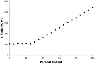
TMS stimulator calibration. The calibration curve for TMS power supply (Cadwell HSMS) is illustrated. X‐axis units are percentage of maximal output, as read from an analog meter on the stimulator. For percent output values greater than 25% the relationship is linear (r2 = 0.9526). TMS intensities used in this study ranged from 30–100% of machine output, well within this linear range.
Imaging Conditions
Each subject underwent two trials of TMS at each of three intensities: two trials of finger tapping (to confirm the location of M1hand), and two trials of sham TMS. The three TMS intensities used were: 75% MT, 100% MT, 125% MT. The different TMS intensities were delivered in pseudo‐randomized order. For the true TMS conditions, TMS was applied at the location previously determined to be the FDI representation within left M1hand. TMS was started 120 s prior to tracer injection and continued through the first 40 s of a 90‐s image acquisition.
Image Acquisition
PET image acquisition procedures are described here briefly, but have been described in detail previously [Fox et al., 2004]. Subjects were scanned using a General Electric (Milwaukee, WI) 4096 whole‐body camera. Mu metal shielding was not employed, as this has been shown unnecessary and lowers image signal‐to‐noise ratio [Fox et al., 1997; Lee et al., 2003; Speer et al., 2003a, b]. Brain blood flow (BF) was measured using 15O‐water, administered as an intravenous bolus. Ninety seconds of data were acquired, triggered by the tracer entering the brain. Throughout the PET session the subjects' heads were immobilized with an individually fitted, thermoplastic facial mask [Fox et al., 1984]. To minimize auditory activation due to the sound emitted by the TMS, foam earplugs were worn throughout the imaging study. Anatomical MRI was acquired in each subject and used to optimize spatial normalization. MR imaging was performed on a 1.9 T, G.E./Elscint Prestige (Haifa, Israel) at a voxel size of 1 mm3.
EMG Acquisition and Processing
Motor evoked potentials were obtained from the FDI contralateral to TMS stimulation. The MEP was obtained from EMG recordings made with a Synamp 1.0 ERP recording system and processed with the Scan 4.0 software (Neuroscan, El Paso, TX). EMG was monitored throughout the period of TMS delivery to ensure effective stimulus delivery. For MEP analysis the first 25 trials obtained during the 40‐s imaging interval were used. For each scan the trials were averaged and quantified as peak‐to‐peak amplitude.
Image Preprocessing
Images were reconstructed into 60 slices, each 2 mm thickness, with an image matrix size of 60 × 128 × 128, using a 5 mm Hann filter resulting in images with a spatial resolution of ∼7 mm (full‐width at half‐maximum (FWHM)). PET images were value normalized to a whole‐brain mean of 1,000. PET and MRI data were coregistered using the Convex Hull algorithm [Lancaster et al., 1999]. MRI data were spatially normalized using the SN [Lancaster et al., 1995] and OSN algorithms [Kochunov et al., 1999] in series. The SN algorithm performed “global” (nine‐parameter) spatial normalization, which registered each subject to the target shape provided by the Talairach and Tournoux [1988] atlas. The OSN algorithm performed “local” spatial normalization, in which each subject's brain was anatomically deformed to match the median of the group in a high‐resolution (1 mm3), fully 3D (each image voxel provides three deformation vectors) manner. OSN processing was used to optimize registration of anatomical features (and thereby functional areas) across subjects. OSN‐derived deformation fields were applied to the PET data prior to computation of statistical parametric images (SPIs).
Image Analysis
Images were analyzed using a combination of voxel‐wise statistical parametric images (SPIs) and volumes‐of‐interest (VOIs). SPIs were computed both per‐subject and for the group. Per‐subject Z‐score images (SPI{z}) contrasting maximal TMS stimulation (125% MT) with the unstimulated control state were used to specify the location of cubic VOIs (1 cm3), which were used to probe the hemodynamic responses at the stimulation site. VOIs were placed at the center‐of‐mass of the left M1hand response, as specified by an automated, local‐maximum search [Mintun et al., 1989]. Three PET‐derived variables were assessed: value normalized counts (VNC), Z‐score, and activation extent. VNC were “raw” PET counts, after normalization of each image to a whole‐brain mean of 1,000. SPI{z} were computed as the contrast of each condition to the sham‐TMS control using an image‐wise standard deviation. The z‐values analyzed were the peak values within the M1hand VOI for each subject in each condition. Extent was computed as the volume (mm3) of response in each SPI{z} above a Z‐value of 1.96 within the M1hand region. In addition, an image of covariance (SPI{r}) was computed group‐wise as the voxel‐wise covariance between ΔVNC and MEP amplitude to illustrate the location and extent of the covariance between hemodynamics and electrophysiology.
Image‐Data Quality Control
Image data from one subject was excluded from analysis due to uncorrectable head movement. MEP data from this subject are included in the 12‐subject group analysis. Four subjects showed no detectable hemodynamic responses to TMS in the M1hand region, even at maximum stimulus intensity, as described in Fox et al. [2004]. Lacking an M1hand response, VOI‐based PET‐data analyses could not be performed on these subjects. Analysis of MEP data was performed in the 12‐subject group and separately in the 7‐subject and 4‐subject groups, as defined by PET response.
Statistical Analysis
The effect of TMS intensity gradations on the four response variables was assessed by repeated‐measures multivariate analysis of variance (MANOVA). For MANOVA and for graphing the two trials obtained per condition per subject were averaged into a single value per condition per subject. For computation of per‐subject correlations and regressions the two trials were kept separate to maximize degrees of freedom. Between‐subject correlations and regressions (e.g., between VNC and MEP) were performed after averaging across stimulus conditions within subject. Statistical analyses were performed using SPSS 11.0 (SPSS, Chicago, IL) and Microsoft Excel X for Mac (Microsoft, Seattle, WA). Graphs were generated with Microsoft Excel X for Mac.
RESULTS
MEP
Recognizable TMS‐driven waveforms were present in 3% of recorded trials (18 of 600) at 75% MT, in 59% of trials (352 of 600) at 100% MT, and in 97% of trials (581 of 600) at 125% MT. In every subject (12/12), MEP amplitude was positively modulated by TMS stimulation intensity. MEP amplitude was low at 75% MT (8.9 μv ± 14.76; mean, ± 1 SEM), slightly stronger at 100% MT (53.2 μv ± 87.89), and much stronger at 125% MT (231.1 μv ± 244.24). Response patterns were similar for PET responders (n = 7; Fig. 2A) and PET nonresponders (n = 4; Fig. 2B). The mean MEP magnitudes (pooling across conditions) for PET responders and PET nonresponders were not significantly different by unpaired t‐test (t = −0.8, P = 0.47).
Figure 2.
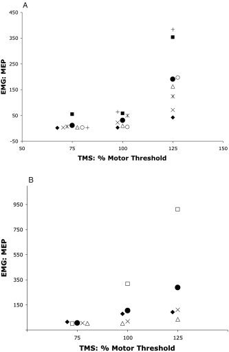
MEP as a function TMS intensity. MEP responses at each stimulation intensity for PET responders (n = 7) are illustrated in A. MEP responses for PET nonresponders (n = 4) are illustrated in B. Filled circles are mean values for each group by condition. Other symbols are for individual subjects. Symbols used for the PET responders (A) are consistent with those used in Figure 3 (below); i.e., the same symbol indicates the same subject. MEP was quantified as peak‐to‐peak amplitude in μV.
The MEP response to intensity modulation was statistically significant both for the 12‐subject pool (F = 7.37, P < 0.005) and for the 7‐subject pool of PET responders (F = 14.9, P < 0.005, Table I). For the 12‐subject and the 7‐subject groups the mean response at 125% MT significantly exceeded the 100% MT response (P < 0.005) and the 100% MT response exceeded the 75% MT response (P < 0.05), by paired t‐test. For the 12‐subject group, regression coefficients for the MEP response to TMS intensity modulation, computed per subject, were all positive and ranged from 0.63 to 0.95, with a mean of 0.79. For these, the P value for the regression was < 0.05 in 6/12, < 0.1 in 9/12, and < 0.2 in 12/12, despite the low degrees of freedom (total df = 5) in this test. The mean regression coefficients for PET responders (0.77 ± 0.04) and nonresponders (0.82 ± 0.06), and were not significantly different by unpaired t‐test (t = 0.7, P = 0.50).
Table I.
Effect of TMS intensity
| Variable | Stimulus Intensity | |||
|---|---|---|---|---|
| 75% MT | 100% MT | 125% MT | F | |
| EMG: MEP | 11 ± 7.3 | 30 ± 9.8 | 190 ± 50.0 | 14.9b |
| PET: ΔVNC | 82 ± 25 | 118 ± 37 | 263 ± 39 | 32.4a |
| PET: Peak Z‐score | 3.81 ± 0.30 | 3.95 ± 0.48 | 5.25 ± 0.51 | 7.4c |
| PET: Extent (mm3) | 778 ± 253 | 2,226 ± 1,255 | 3,556 ± 1,317 | 6.0c |
Values reported are ± 1 SEM. For all variables, n = 7.
F‐statistics are for within‐subject contrasts:
P < 0.0005;
P < 0.005;
P < 0.05.
The magnitude of the effect on M1hand cortex of TMS intensity modulation varied across measurement variables. The strongest effects were on VNC and MEP. Effect significance was determined by repeated‐measured MANOVA with TMS intensity as the within‐subject factor.
Stimulation‐Site PET Responses
Three‐Hertz TMS increased BF at the stimulated site (left M1hand representation) in seven subjects. All three of the PET‐measured variables showed statistically significant effects of TMS stimulation (Table I). The most robust effect was in VNC (F = 32.4, Table I). Less robust but significant effects were observed in peak Z‐score and response extent (Table I). For VNC, the mean response at 125% MT significantly exceeded the 100% MT response (t = 6.4, P < 0.0005); however, the 100% MT response did not significantly exceed the 75% MT response (t = 0.1, P > 0.1) by paired t‐test.
The trend of the intensity‐response functions for VNC (Fig. 3) was the same as for the MEP intensity‐response function (Fig. 2). As with MEP, 75% MT and 100% MT stimulation induced relatively weak responses, while 125% MT stimulation produced very robust responses. Correlation coefficients expressing covariance between VNC and TMS intensity computed per subject were all positive and ranged from 0.58–0.96, with a mean of 0.75. Of these, the P value (of the regression) was < 0.05 in 5/7 subjects and < 0.15 in 7/7, despite the low degrees of freedom (total df = 7) in this test.
Figure 3.
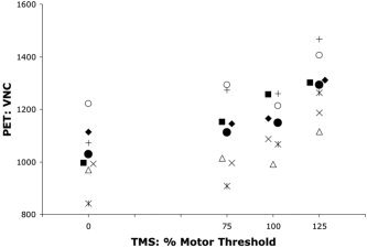
PET blood flow (BF) responses. PET BF responses (VNC) at the stimulated site (M1hand) for each stimulation intensity are illustrated for the seven PET responders. Filled circles are mean values for the group by condition. Other symbols indicate individual subjects. Symbols used are consistent with those used in Figure 2A; i.e., the same symbol indicates the same subject.
PET:EMG Covariation
Significant covariance was observed between the PET‐measured hemodynamic responses and the EMG‐measured electrophysiological response, both within and between subjects (Fig. 4). In all seven subjects the per‐subject correlations between VNC and MEP computed per subject were positive and ranged from 0.33–0.88, with a mean of 0.66. Of these, the P value (of the regression) was < 0.05 in 2/7 and < 0.2 in 6/7, despite the low degrees of freedom (total df = 5). The between‐subjects correlation coefficient was 0.76, which achieved statistical significance (F = 6.8, P < 0.05, total df = 6). The correlation coefficient computed pooling between‐ and within‐subjects effects was highly significant (r = 0.60, F = 22.9, P < 0.00005, total df = 41). The group SPI{r} computed as the voxel‐wise correlation between MEP and VNC (Fig. 5) illustrates that the covariance between hemodynamics and electrophysiology was localized to the stimulated region. The maximum r value in the M1hand region of the SPI{r} was 0.61 at an x‐y‐z address of −32, −30, 48 [Talairach and Tournoux, 1988].
Figure 4.
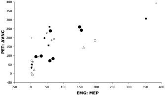
Scatterplot of hemodynamic and electrophysiological responses. The relation between PET blood‐flow responses at the stimulated site (M1hand) and MEP is illustrated for the seven PET responders. Filled circles are mean responses for each subject, pooling across conditions to illustrate the between‐subjects correlation of PET (ΔVNC) and EMG (MEP). Other symbols indicate individual subjects, illustrating the within‐subject effect of TMS intensity on both hemodynamics and electrophysiology. PET responses were quantified as the change in value normalized counts (ΔVNC) from the unstimulated baseline state. MEP was quantified as peak‐to‐peak amplitude in μV.
Figure 5.
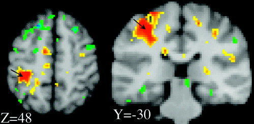
PET blood flow (BF) response. Images shown are sections from an SPI{r} computed as voxel‐wise covariance with per‐subject MEP (peak‐to‐peak amplitude) as the pattern vector. At the stimulation site (arrows), hemodynamic and electrophysiological response functions were highly correlated. Maximum positive covariance was at the stimulated site and was r = 0.61 (peak voxel), at an x‐y‐z address of −32, −30, 48. Orange and red hues indicate positive covariances; blue and green hues indicate negative covariances. Scale ranges are: 0.30 < r < 0.60; and −0.30 > r > −0.60.
Remote Stimulus‐Response Functions
Significant covariation with the M1hand hemodynamic stimulus‐response function was observed in numerous regions. Stimulus‐response profiles for the four regions in which BF changes correlated most strongly (either positively or negatively) with BF responses in M1hand are illustrated (Fig. 6). These were: left cingulate gyrus; left supplementary motor area (SMA); right cerebellum (CBM); and right M1hand. Two basic response patterns were seen: a ramp function and a step function. The cingulate response was a rising ramp function, closely resembling the M1hand MEP (Fig. 2) and PET (Fig. 4) responses. The cerebellar response was a ramp function with a negative slope, effectively the inverse of the M1hand and cingulate responses. The SMA response was a positive step function; the right M1hand was a negative step function.
Figure 6.
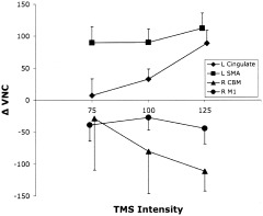
Remote responses: VOI data. PET VOI data are plotted for the four regions in which blood‐flow changes correlated most strongly (either positively or negatively) with blood‐flow responses in M1hand: left cingulate gyrus; left SMA; right cerebellum; right M1hand. PET responses were quantified as the change in value normalized counts (ΔVNC) from the unstimulated baseline state. All plotted values are means (n = 7). Error bars are ± 1 SEM.
DISCUSSION
Stimulus‐response functions for PET‐measured hemodynamic variables and MEP amplitude were similar. For all response variables response functions were nonlinear, with a more rapid rate of rise above motor threshold than below. VNC was the hemodynamic response variable showing the most significant modulation by stimulus intensity. VNC and MEP were significantly correlated both between and within subjects, indicating that VNC is a reasonable surrogate for electrophysiology for stimulus‐response profile characterization. In the four remote regions assessed, stimulus‐response profiles varied both in slope sign (+ or −) and in shape, reflecting variations not only in the valence of the neural projection (excitatory vs. inhibitory) but also in the stimulus‐response profile of the connected regions.
Electrophysiological Intensity‐Response Functions
MEP results obtained here are reasonably consistent with those of Capaday and colleagues [Devanne et al., 1997; Capaday, 1997; Capaday, 2004]. Using MEP recordings, Capaday demonstrated that the primary motor cortex (M1) stimulus‐response profile to intensity‐graded TMS is a sigmoid function, with a ceiling level at which the response saturates and a floor below which there is no measurable effect. Acquiring single‐motor‐unit recordings under similar conditions, Capaday further demonstrated that the probability of firing of individual motor units is a linear function of TMS intensity. From these observations it was suggested that the stimulus‐response curve reflected population‐level variables related to the recruitment of cortical and spinal neurons. The present results are consistent with Capaday's results in finding a nonlinear response with a slowly rising “floor” region at lower intensities and a more steeply rising segment at higher stimulation intensities. However, the present results fail to demonstrate a clear ceiling effect. The absence of a ceiling effect in our results is most likely explained by three factors. First, the maximum stimulus intensity used here was less than that used by Capaday. Capaday's subjects were stimulated at 100% of machine output (MO) and at 10% decrements therefrom (90% MO, 80% MO, etc.). Our subjects were stimulated at a maximum value of 125% MT, which was variable relative to percent MO, reflecting individual variations in motor threshold. In our subjects, 125% MT averaged 86.5% MO (range 68.8–100%). Second, our subjects were studied only at rest; they made no voluntary muscle contractions during TMS stimulation. Capaday demonstrated that the steepness of the intensity response function and the prominence of the ceiling effect were functions of the degree of preloading of the muscle (i.e., the force of voluntary contraction during stimulation). In the resting state, Capaday's ceiling value for FDI was ∼90% MO, indicating that we fell just short of achieving ceiling. Third, we applied only a single stimulation intensity near the ceiling value, although we applied two intensities near the floor value. If we had obtained two values near ceiling, our proximity to ceiling could have been demonstrated. Because of the lack of a ceiling effect and the small number (3) of stimulus‐intensity values sampled, we could not apply Capaday's model to the present dataset. However, we have replicated Capaday's MEP results in a small subject sample (n = 5) and are in the process of acquiring a TMS‐PET dataset with broader sampling by intensity.
As indicated above, Capaday and colleagues proposed that the excitability of cortical neural populations can be characterized by the TMS stimulus‐response profile and that the stimulus‐response profile can be related to the resting‐state distribution of excitability in the neuronal population recruited by the TMS pulse. In this construct, Capaday used a mathematical model derived from the Boltzman equations, relating firing probability to shift in excitability. Komssi et al. [2004] extended this modeling construct by making the explicit argument that the effect of TMS can be modeled as shifting the membrane potential relative to the depolarization threshold. The graded stimulus‐response profile reflects the bell‐shaped, resting‐state distribution of neuronal membrane potentials relative to the depolarization threshold [Komssi et al., 2004, fig. 1]. Thus, the sigmoid function is the cumulative population recruitment, while its bell‐shaped first derivative reflects the membrane‐potential distribution. In the same publication, Komssi et al. extended Capaday's stimulus‐response modeling construct to ERP, stimulating M1hand at 60, 80, 100, and 120% MT and obtained a global mean field amplitude (GMFA) response function [Komssi et al., 2004, fig. 5]. Komssi et al.'s GMFA response function is quite similar to the MEP function reported here (Fig. 2A,B). As in the present study, Komssi did not use preloading of the muscle. Also as in the present study, Komssi et al. found a floor effect but not a ceiling effect, likely for the reasons given above.
M1 Blood Flow Response: Sign
The hemodynamic response in M1hand during 3‐Hz TMS stimulation was an increase in local BF (Fig. 3). Increased M1hand BF was observed in all seven subjects showing an M1hand response and at all three intensities. In no instance did we observe a decrease in BF below baseline at the stimulation site. (For details on per‐subject M1hand responses, see Fox et al. [2004].) The observation of increased BF in M1hand during TMS stimulation is in agreement with most, but not all, of the relevant literature. Increased local BF during M1hand stimulation was reported by Fox et al. [1997] using 1‐Hz TMS at 120% MT in a H2 15O‐PET experiment; by Bohning et al. [1999] using 1‐Hz TMS at 80% and 100% MT in a block‐design, BOLD fMRI experiment; by Bohning et al. [2000] using single‐pulse TMS at 120% MT, in an event‐related fMRI experiment; by Siebner et al. [2001] using 90% MT stimulation at rates between 1 Hz and 5 Hz in a H2 15O‐PET experiment; and by Speer et al. [2003a] using 1‐Hz TMS at intensities ranging from 80–120% MT. The sole report of decreased local BF during TMS stimulation of M1hand is a H2 15O‐PET study by Paus et al. [1998]; the reasons for this discrepancy are unclear.
M1 Hemodynamic Response Variables
Hemodynamic responses can be quantified and assessed for statistical significance both by intensity and by extent [Xiong et al., 1999]. Of the response variables reported here (Table I), Z‐score most purely measures response intensity, while volume most purely measures response extent. Increases in response intensity most likely reflect increases in the fraction of neurons, within a fixed volume, that have been excited by the stimulus. Increases in response extent most likely reflect the increase in brain volume exposed to a supra‐threshold level of stimulation as the TMS‐induced magnetic field expands. It may also reflect increased recruitment of horizontal connections of M1 [Capaday, 2004]. Value‐normalized counts (VNCs) measured within a single voxel reflect response intensity. However, VNC measured within a VOI is a mixed measurement, being affected by both intensity and extent. While response intensity (z‐score) and response extent (mm3) were significantly modulated by TMS intensity (Table I), intensity showed the stronger effect. This is in agreement with the model proposed by Capaday and colleagues, by which intensity‐based modulation of the TMS‐induced response is attributed to an increase in the fraction of the neurons being excited. VNC was the hemodynamic variable most strongly modulated by TMS, with a much more significant effect than either intensity or extent. The magnitude of the difference is rather surprising, with VNC having an F‐value 4–5 times greater than intensity or extent (Table I). In part, this can be attributed to the conjoined effects of intensity and extent. Another likely factor is that VNC is the most direct measure of the hemodynamic response, requiring no additional computations or data manipulations.
A hemodynamic response function for TMS stimulation intensity of M1 was reported by Speer et al. [2003a] for TMS‐intensity values of 80%, 90%, 100%, 110%, and 120% MT. Although acquired with 1 Hz TMS, Speer et al.'s hemodynamic response function for M1 is similar to that reported here. Expressed in percent change over baseline, Speer et al. observed changes ranging from ∼3% (80% MT) to ∼11% (120% MT). The percent changes we observed ranged from 5% (75% MT) to 14% (125% MT) using 3‐Hz stimulation. The similarity of the values, despite the difference in stimulation rate, is somewhat unexpected. The effect of stimulation rate on hemodynamic response magnitude is very well established, for both PET [Fox and Raichle, 1984, 1985; Fox et al., 2002] and fMRI [Kwong et al., 1992; Schneider et al., 1993], giving nearly identical rate‐response functions across modality. The source of the linear component of the rate‐response function is believed to be simple temporal integration, averaging more neural events per scan epoch at higher stimulation rates [Fox and Raichle, 1984]. A linear rate‐response function for TMS has been reported using 15O‐PET by Siebner et al. [2001], demonstrating that TMS is not an exception to the rate‐response rule. One possible explanation of the unexpected similarity of response magnitude is the superior spatial resolution of the PET camera used by Speer et al. (Siemens HR+, spatial resolution ∼4 mm) relative to our (GE 4096, spatial resolution ∼7 mm).
Covariance of Hemodynamics and Electrophysiology
MEP and VNC were correlated by within‐subject analysis, by between‐subject analysis, and by a mixed within‐ and between‐subject analysis. The within‐subject analysis most purely reflects the similarity of the effect of variations of TMS intensity on both types of response variable, hemodynamic and electrophysiological. The present study is the first (to our knowledge) to compare a hemodynamic response function to an electrophysiological response function during intensity‐graded TMS stimulation. However, two other TMS reports do provide a basis for comparison. First, Strafella and Paus [2001] varied interpulse interval in a paired‐pulse TMS experiment as a means of manipulating the MEP magnitude; covariance with PET‐measured BF responses were significant (P < 0.01) for M1 (the stimulated site), as well as for connected regions. Second, Komssi et al. [2004] reported GMFA during TMS intensity modulation (discussed above); the GMFA function closely resembles the MEP and hemodynamic functions reported here.
The between‐subjects correlation analysis, by averaging across stimulus intensities within subject, demonstrates that intersubject variations in response strength are correlated for both types of response variable. It is well known in the functional brain imaging community that some subjects are “strong responders,” while others are “weak responders.” The between‐subjects comparison demonstrates that response strength was highly correlated across modalities. “Strong responders” for PET were also “strong responders” for MEP; “weak responders” for PET were also “weak responders” for MEP. It is important to note that the “strong responder / weak responder” effect does not explain the four PET nonresponders, as there was no difference in mean MEP magnitude or in the mean “r” value of the regression of MEP with stimulus intensity between PET responders and PET nonresponders. Thus, there must be some other explanation for the nonresponders, as follows.
The electrophysiological measurement employed here, MEP, reflects corticospinal neuron output from M1. Logothetis et al. [2001] compared multiunit activity (MUA; a measure of spike output) and local field potentials (LFP, a measure of input and local intracortical processing) with BOLD fMRI (a measure of the hemodynamic response) in monkey visual cortex. Both electrophysiological measures correlated very strongly with the BOLD signal. For MUA, mean r2 = 0.445 (r = 0.67); for LFP, mean r2 = 0.522 (r = 0.721). In the present study, the average per‐subject correlation between H2 15O PET VNC (reflecting blood flow) and MEP (reflecting spike output) had an r2 = 0.435 (r = 0.66), which is virtually identical to the Logothetis et al. value for MUA. Because the correlation with the hemodynamic response was slightly (but significantly) higher for LFP than for MUA, Logothetis et al. [2001] suggested that the hemodynamic response “reflects the input and intracortical processing of a given area rather than its spiking output” (p 154). They went on to predict that if the two electrophysiological measures could be dissociated, the hemodynamic response would follow input rather than output. We hypothesize that the four PET nonresponders are an example of such a circumstance. In each of the four subjects in whom no local hemodynamic response was observed during TMS stimulation, the EMG response was present and indistinguishable from that of the PET responders. This may well be caused by direct stimulation of the exiting corticospinal axon, causing excitation of the corticospinal fibers but not of the gray matter. The way to address this issue is with prospective experiments using a spatially precise, image‐guided TMS positioning system, as has been described by Lancaster et al. [2004], and in the context of a well‐defined aiming theory [Fox et al., 2004].
Remote‐Region Intensity‐Response Functions
Intensity modulation of TMS delivered to M1hand was highly effective at producing remote covariances with the stimulated site. The connectivity map for M1hand based on these covariances will be addressed in a subsequent article. Here, stimulus‐response profiles are reported for four regions that exhibited strong covariance with M1hand (Fig. 6): the two regions with the strongest positive covariance (ipsilateral anterior cingulate and ipsilateral SMA) and the two regions with the strong negative covariance (contralateral cerebellum and contralateral M1hand). That the projection of M1hand to its contralateral homolog is inhibitory, for example, has been well established by TMS/EMG [Wasserman et al., 2000]. Accordingly, we interpret the negative covariances as indicative of inhibitory projections from the stimulated M1hand region and the positive covariances as indicative of excitatory projections. Although all four regions significantly correlated with the M1hand response, all four differed in their response profiles from one another and from M1hand. Of the two regions with positive covariance, one exhibited a fairly linear rise with stimulation intensity (anterior cingulate), while the other (SMA) showed a low threshold and a ceiling effect. Of the two regions with the strongest negative covariance, M1hand (strongest negative covariance with M1hand) showed response profiles that were inverted but otherwise similar: one was linear (cerebellum). We interpret the varied response profiles as possibly reflecting different levels of neuronal excitability. Whether the response profiles derived from stimulating an area via its connectivity will be the same as from stimulating it directly remains to be determined. One possibility is that the response profile of a remote region is the convolution of the two response profiles: stimulated site and remote site. This can only be determined prospectively, with additional experiments. If so, it suggests that stimulus‐response profiles could be obtained for brain areas that cannot be stimulated directly with TMS.
Intensity‐Graded Connectivity Mapping
Combined application of TMS and functional imaging is one of the most promising strategies for mapping interregional brain connectivity. When imaging is used in combination with TMS to assess interregional connectivity, the existence and strength of neuronal connections between a stimulated region and a remote region can be quantified by the strength of covariance between the regions. In this experimental scenario the most robust assessment of connectivity will be obtained when a TMS stimulation parameter is exploited as a means of increasing the range of the induced responses. For optimal efficacy, the stimulation parameter varied should have a more or less linear effect on the induced responses, both locally and remotely. Additionally, the dynamic range of the stimulation parameter must be known and exploited, to guarantee good sampling of the response function. Based on these considerations, we would argue that intensity is an important physiological variable for connectivity mapping, but one that has not yet been used optimally for this purpose. Although intensity‐graded TMS has been combined with functional imaging to map connectivity [e.g., Nahas et al., 2001; Speer et al., 2003a, b], no group, including ourselves, has fully exploited the range of this variable as demonstrated by Devanne et al. [1997]. Rather, stimulation has been limited to the middle and lower portions of the stimulus‐response function. We would suggest extending the stimulation range from floor to ceiling, simultaneously enhancing both the analysis of interregional covariance and the modeling of stimulus‐response functions. In motor cortex, the appropriate range of intensities could be determined with EMG prior to imaging; in nonmotor cortex, GMFA would be an appropriate calibration technique. Further, voluntary recruitment of the stimulated region during stimulation should be explored as a strategy for lowering the intensity of stimulation needed to reach the response ceiling [Devanne et al., 1997].
Acknowledgements
We thank John Roby for modifications to the Cadwell HSMS unit and to the PET scanner that facilitated the performance of this experiment. We thank Crystal Franklin and Neil Murthy for analysis of PET and EMG data. We thank David Glahn, Larry Price, and Thomas Coyle for critique of the statistical analyses performed.
REFERENCES
- Bohning DE, Pecheny AP, Epstein CM, Speer AM, Vincent DJ, Dannels W, George MS (1997): Mapping transcranial magnetic stimulation (TMS) fields in vivo with MRI. Neuroreport 8: 2535–2538. [DOI] [PubMed] [Google Scholar]
- Bohning DE, Shastri A, McConnell KA, Nahas Z, Lorberbaum JP, Roberts DR, Teneback C, Vincent DJ, George MS (1999): A combined TMS/fMRI study of intensity‐dependent TMS over motor cortex. Biol Psychiatry 45: 385–394. [DOI] [PubMed] [Google Scholar]
- Bohning DE, Shastri A, Wassermann EM, Ziemann U, Lorberbaum JP, Nahas Z, Lomarev MP, George MS (2000): BOLD‐fMRI response to single‐pulse transcranial magnetic stimulation (TMS). J Magn Reson Imaging 11: 569–574. [DOI] [PubMed] [Google Scholar]
- Capaday C (1997): Neurophysiological methods for studies of the motor system in freely moving human subjects. J Neurosci Methods 74: 201–218. [DOI] [PubMed] [Google Scholar]
- Capaday C (2004): The integrated nature of motor cortical function. Neuroscientist 10: 1–14. [DOI] [PubMed] [Google Scholar]
- Devanne H, Lavoie BA, Capaday C (1997): Input‐output properties and gain changes in the human corticospinal pathway. Exp Brain Res 114: 329–338. [DOI] [PubMed] [Google Scholar]
- Fox PT, Raichle ME (1984): Stimulus rate dependence of regional cerebral blood flow in human striate cortex, demonstrated by positron emission tomography. J Neurophysiol 51: 1109–1120. [DOI] [PubMed] [Google Scholar]
- Fox PT, Raichle ME (1985): Stimulus rate determines regional brain blood flow in striate cortex. Ann Neurol 17: 303–305. [DOI] [PubMed] [Google Scholar]
- Fox PT, Ingham RJ, Mayberg H, George M, Martin C, Ingham J, Robey J, Jerabek P (1997): Imaging human cerebral connectivity by PET during TMS. Neuroreport 8: 2787–2791. [DOI] [PubMed] [Google Scholar]
- Fox PT, Ingham RJ, Ingham JC, Zamarripa F, Xiong J‐H, Lancaster JL (2002): Brain correlates of stuttering and syllable production. Brain 123: 1985–2004. [DOI] [PubMed] [Google Scholar]
- Fox PT, Narayana S, Tandon N, Sandoval H, Fox SP, Kochunov P, Lancaster JL (2004): Column‐based model of electric field excitation of cerebral cortex. Hum Brain Mapp 22: 1–14. [DOI] [PMC free article] [PubMed] [Google Scholar]
- Ilmoniemi RJ, Virtanen J, Ruohonen J, Karhu J, Aronen HJ, Naatanen R, Katila T (1997): Neuronal responses to magnetic stimulation reveal cortical reactivity and connectivity. Neuroreport 8: 3537–3540. [DOI] [PubMed] [Google Scholar]
- Kochunov PV, Lancaster JL, Fox PT (1999): Accurate high‐speed spatial normalization using an octree method. Neuroimage 10: 724–737. [DOI] [PubMed] [Google Scholar]
- Komssi S, Kahkonen S, Ilmoniemi RJ (2004): The effect of stimulus intensity on brain responses evoked by transcranial magnetic stimulation. Hum Brain Mapp 21: 154–164. [DOI] [PMC free article] [PubMed] [Google Scholar]
- Belliveau JW, Kwong KK, Kennedy DN, Baker JR, Stern CE, Benson R, Chesler DA, Weisskoff RM, Cohen MS, Tootell RB, et al. (1992): Dynamic magnetic resonance imaging of human brain activity during primary sensory stimulation. Proc Natl Acad Sci U S A 89: 5675–5679. [DOI] [PMC free article] [PubMed] [Google Scholar]
- Lancaster JL, Glass TG, Lankipalli BR, Downs H, Mayberg H, Fox PT (1995): A modality‐independent approach to spatial normalization of tomographic images of the human brain. Hum Brain Mapp 3: 209–223. [Google Scholar]
- Lancaster JL, Fox PT, Downs JH, Nickerson D, Hander T, El Mallah M, Zamarripa F (1999): Global spatial normalization of the human brain using convex hulls. J Nucl Med 40: 942–955. [PubMed] [Google Scholar]
- Lancaster JL, Narayana S, Wenzel D, Luckemeyer J, Roby J, Fox PT (2004): Evaluation of an image‐guided robotically‐positioned transcranial magnetic stimulation system. Hum Brain Mapp 22: 329–340. [DOI] [PMC free article] [PubMed] [Google Scholar]
- Lee JS, Narayana S, Lancaster J, Jerabek P, Lee DS, Fox PT (2003): Positron emission tomography during transcranial magnetic stimulation does not require micro‐metal shielding. Neuroimage 19: 1812–1819. [DOI] [PubMed] [Google Scholar]
- Logothetis NK, Pauls J, Augath M, Trinath T, Oeltermann A (2001): Neurophysiological investigation of the basis of the fMRI signal. Nature 412: 150–157. [DOI] [PubMed] [Google Scholar]
- Mintun MA, Fox PT, Raichle ME (1989): A highly accurate method of localizing regions of neuronal activation in the human brain with positron emission tomography. J Cereb Blood Flow Metab 9: 96–103. [DOI] [PubMed] [Google Scholar]
- Nahas Z, Lomarev M, Roberts DR, Shastri A, Lorberbaum JP, Teneback C, McConnell K, Vincent DJ, Li X, George MS, Bohning DE (2001): Unilateral left prefrontal transcranial magnetic stimulation (TMS) produces intensity‐dependent bilateral effects as measured by interleaved BOLD fMRI. Biol Psychiatry 50: 712–720. [DOI] [PubMed] [Google Scholar]
- Paus T, Jech R, Thompson CJ, Comeau R, Peters T, Evans AC (1997): Transcranial magnetic stimulation during positron emission tomography: a new method for studying connectivity of the human cerebral cortex. J Neurosci 17: 3178–3184. [DOI] [PMC free article] [PubMed] [Google Scholar]
- Paus T, Jech R, Thompson CJ, Comeau R, Peters T, Evans AC (1998): Dose‐dependent reduction of cerebral blood flow during rapid‐rate transcranial magnetic stimulation of the human sensorimotor cortex. J Neurophysiol 79: 1102–1107. [DOI] [PubMed] [Google Scholar]
- Schneider W, Casey BJ, Noll D (1994): Functional MRI mapping of stimulus rate effects across visual processing stages. Hum Brain Mapp 1: 117–133. [Google Scholar]
- Siebner HR, Takano B, Peinemann A, Schwaiger M, Conrad B, Drzezga A (2001): Continuous transcranial magnetic stimulation during positron emission tomography: a suitable tool for imaging regional excitability of the human cortex. Neuroimage 14: 883–890. [DOI] [PubMed] [Google Scholar]
- Speer AM, Willis MW, Herscovitch P, Daube‐Witherspoon M, Shelton JR, Benson BE, Post RM, Wassermann EM (2003a): Intensity‐dependent regional cerebral blood flow during 1‐Hz repetitive transcranial magnetic stimulation (rTMS) in healthy volunteers studied with H215O positron emission tomography. I. Effects of primary motor cortex rTMS. Biol Psychiatry 54: 818–825. [DOI] [PubMed] [Google Scholar]
- Speer AM, Willis MW, Herscovitch P, Daube‐Witherspoon M, Shelton JR, Benson BE, Post RM, Wassermann EM (2003b): Intensity‐dependent regional cerebral blood flow during 1‐Hz repetitive transcranial magnetic stimulation (rTMS) in healthy volunteers studied with H215O positron emission tomography. II. Effects of prefrontal cortex rTMS. Biol Psychiatry 54: 826–832. [DOI] [PubMed] [Google Scholar]
- Strafella AP, Paus T (2001): Cerebral blood‐flow changes induced by paired‐pulse transcranial magnetic stimulation of primary motor cortex. J Neurophysiol 85: 2624–2629. [DOI] [PubMed] [Google Scholar]
- Talairach J, Tournoux P (1988): Coplanar stereotactic atlas of the human brain. 3‐Dimensional proportional system: an approach to cerebral imaging. Stuttgart, Germany: Thieme. [Google Scholar]
- Wasserman EM, Fuhr P, Cohen LG, Hallett M (2000): Effects of transcranial magnetic stimulation on ipsilateral muscles. Neurology 41: 1785–1789. [DOI] [PubMed] [Google Scholar]
- Xiong J, Parsons LM, Gao JH, Fox PT (1999): Interregional connectivity to primary motor cortex revealed using MRI resting state images. Hum Brain Mapp 8: 151–156. [DOI] [PMC free article] [PubMed] [Google Scholar]